Eddy-induced sea surface salinity changes in the South China Sea

1 Introduction

More than 50% of the variability over much of the world’s ocean is accounted for by eddies (Chelton et al., 2011). Nonlinear eddies can significantly impact the redistribution of oceanic tracers and energy through horizontal and vertical transport (Melnichenko et al., 2021; Guo and Bishop, 2022) and play an essential role in modulating ocean mean circulation and its variability (Storch et al., 2012; Guo et al., 2022). As a tropical marginal sea connecting the Indo-Pacific oceans, the South China Sea (SCS) features vigorous mesoscale eddy activity. Previous studies have examined the statistical characteristics of eddies (Wang et al., 2003; Xiu et al., 2010; Chen et al., 2011; He et al., 2018), their influence on near-sea-surface characteristics (He et al., 2016; Sun et al., 2018; He et al., 2019) and their induced ocean tracer transport in the SCS (Chen et al., 2012; Yang et al., 2019; Ding et al., 2021; Yang et al., 2021).

Sea surface salinity (SSS) is one of the important physical parameters of the global water cycle, profoundly influencing the thermal and dynamic structural characteristics of the ocean (Durack, 2015). Zeng et al. (2019) suggested a high correlation between springtime SSS in the central SCS and summer precipitation over the middle and lower Yangtze River Valley. Analyses show that the SCS is one of the lowest SSS areas that experienced the most significant freshening during the 1950–2000 period (Durack et al., 2012; Zeng et al., 2014). On the other hand, the SCS Throughflow brings a large amount of saline Kuroshio water through the Luzon Strait, which contributes to salinity variations in the SCS to some extent (Qu et al., 2006; Gordon et al., 2012). The spatial relationship between eddy kinetic energy (EKE) and SSS is shown in Figure 1, where high EKE occurs in the western boundary flow area and west of the Luzon Strait. EKE maps are computed using the formula $EKE=\frac{1}{2}(u{\text{'}}_g^2+v{\text{'}}_g^2)$ where $u_g^{\text{'}}$ and $v_g^{\text{'}}$ indicate meridional and zonal geostrophic velocity anomalies, respectively. To date, studies have confirmed the capability of eddies to transport saline Kuroshio water into the SCS (Jia and Liu, 2004; Zhang et al., 2017; Yang et al., 2019; Yang et al., 2021).

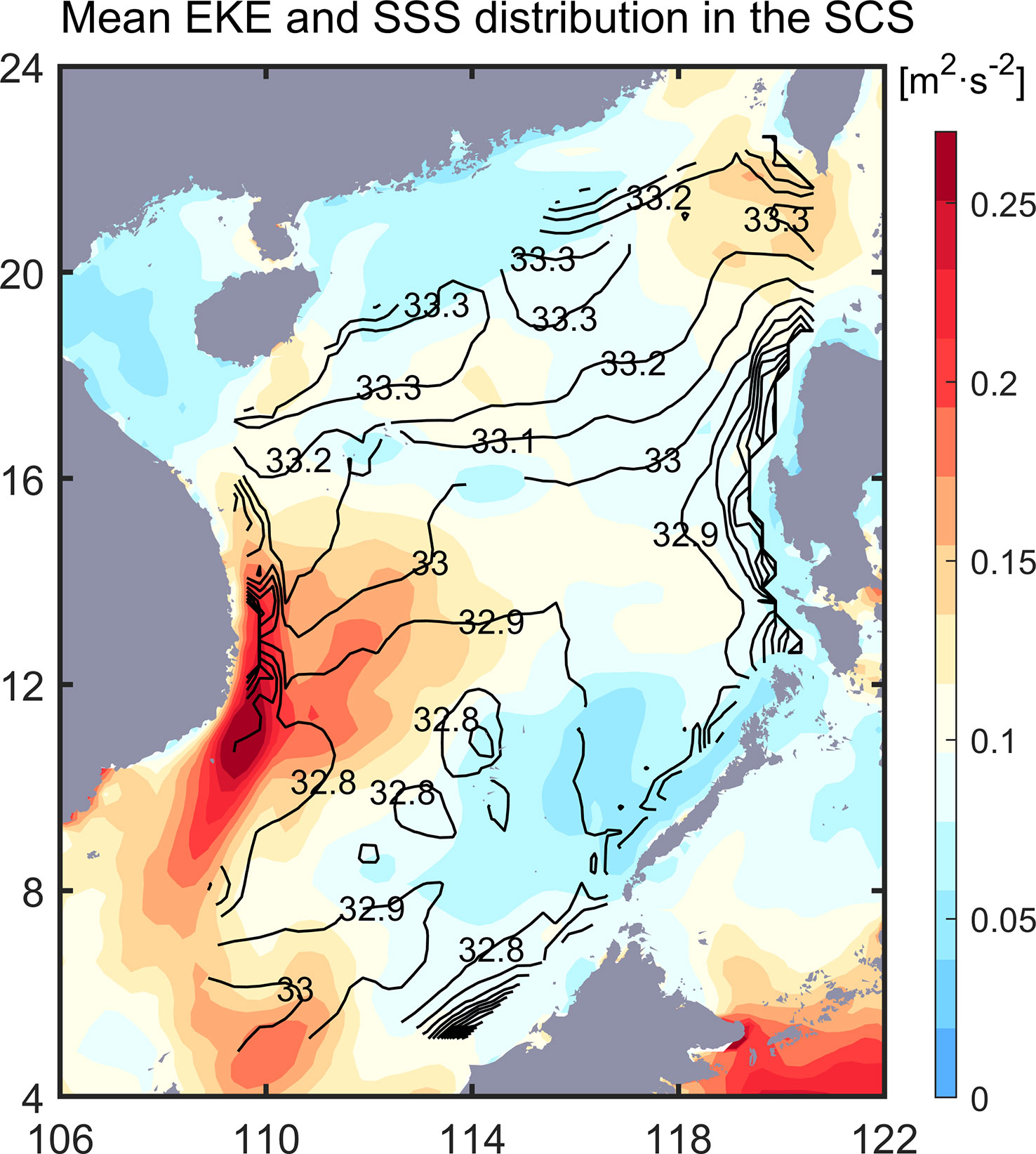
Figure 1 Seven-year (2015-2021) averaged EKE (shading, unit: m²·s^-2) and SSS (black contours, unit: psu) distributions in the SCS.

For many years, only a few studies have investigated the mesoscale variability in SSS based on ship measurements due to the lack of high-resolution observational data (Delcroix et al., 2005; Boutin et al., 2016). Using Argo profiles, He et al. (2018) evaluated the surface features and 3-D structures of mesoscale eddies in the SCS. However, traditional observations do not have high spatial and temporal resolutions and sufficient regional coverage. In recent years, satellite observations with global coverage have greatly enriched our knowledge of the variability in global SSS. For example, the Soil Moisture and Ocean Salinity (SMOS) mission was conducted by the European Space Agency (ESA) in 2010 (Kerr et al., 2010). The Aquarius mission of the National Aeronautics and Space Administration (NASA) and the Soil Moisture Active Passive (SMAP) observation program, which are primarily focused on monitoring land conditions, can still be used to invert SSS data. With satellite salinity data derived from the Aquarius, the correlation between mesoscale eddies and SSS variations was studied in the Gulf Stream region (Umbert et al., 2015), Mediterranean Sea (Isern-Fontanet et al., 2016), South Indian Ocean and North Atlantic subtropical sea regions (Melnichenko et al., 2017), and tropical Pacific Ocean (Delcroix et al., 2019). Using Aquarius satellite salinity data, Umbert et al. (2015) showed that negative salinity anomalies coincide well with the locations of cyclonic eddies identified based on sea level anomalies. Melnichenko et al. (2017), using SMOS satellite salinity data, showed that the typical salinity anomaly of the eddy composite is 0.03-0.05 psu in the southern Indian Ocean and North Atlantic subtropical region. Delcroix et al. (2019) showed a dipole (monopole) mode in the central (eastern) tropical Pacific Ocean by analyzing the structure of the salinity anomalies of the eddy composite.

In summary, a thorough investigation of eddy-induced salinity anomaly patterns has yet to be discovered with eddy-permitting consistent observations in the SCS. This study aims to analyze the SSS changes modulated by eddies with SMAP satellite data and historical in situ observations from 2015 to 2021. This paper is organized as follows: section 2 describes the satellite and eddy datasets and the eddy composite methods; section 3 presents the results of the spatial and seasonal characteristics of the eddy salinity anomaly; section 4 is a discussion of the dipole/monopole patterns of eddy-induced salinity anomaly; and finally, a summary is provided in section 5.

2 Data and methodology

2.1 Datasets

The satellite observations, in situ hydrographic profiles, and an eddy-census dataset used in this work are summarized in this section.

1) The 8-day averaged SMAP satellite L3 salinity product is used in this study with spatial and temporal resolutions of 1 day and 0.25°, respectively, spanning from January 2015 to December 2021. The satellite salinity data products are obtained based on NASA’s SMAP satellite observations and produced with remote sensing systems. To obtain mesoscale SSS variability signals, 6° × 6° 2D Gaussian and 10-120 day bandpass filtering is conducted on the salinity data (Melnichenko et al., 2017; Delcroix et al., 2019). Such filtering will retain eddy-induced SSS changes (i.e., SSS anomalies) and remove the large-scale and seasonal signals that are not associated with eddies. Simultaneous daily averaged Archiving, Validation and Interpretation of Satellite Oceanographic data (AVISO) sea surface geostrophic current anomaly data are also used, which share the same temporal and spatial resolution with the salinity data mentioned above in 2015-2021.

2) Eddy products for 2015-2021 are based on the scale-selective eddy identification algorithm (SEIA), which is SLA-based (Yang et al., 2023, under review). SEIA uses a scale-selective scheme, which restricts the eddy boundary based on the data resolution and eddy spatial scale. During the detection, one-core eddies with radii smaller than the dataset resolution (0.25° in this work) are removed and the eddy boundary is constrained by a scale parameter. The tracking process of SEIA is based on the overlap rate of time-continuous eddies which can effectively guarantee the continuity of the eddy movement path. The validation of eddy statistical features and mesoscale eddy effects based on the SEIA output confirms its effectiveness (Yang et al., 2023, under review). Over 7 years, approximately 24,000 specific eddies existed within the SCS based on daily detection, with a nearly 1:1 ratio of anticyclonic eddies (AEs) to cyclonic eddies (CEs). Weak and abnormal eddies with radii of less than 0.5° are removed considering their trivial effect on local transport and energetics (Xiu et al., 2010; Chen et al., 2011).

The distribution of the number of eddies is shown in Figure 2. To couple the satellite salinity data, eddies with lifetimes shorter than 10 days are also removed. Distinguished by red and blue colors, the AEs and CEs cover the entire SCS, with a total number up to approximately 120 in each 0.5°×0.5° geographical grid over 7 years. A larger number of eddies is mainly distributed to the west of the Luzon Strait, the middle of the basin and offshore Vietnam, which is consistent with previous studies (Wang et al., 2003; Xiu et al., 2010; Chen et al., 2011; He et al., 2018). As shown in the histogram, under a Euler perspective, more eddies are found in boreal spring and summer, and fewer eddies exist in autumn, with a difference of approximately 4000 eddies in the entire basin (Figure 2C). The numbers of the two types of eddies are similar in each season, but the overall number of AEs is slightly higher (AE 9766: CE 9011). Figures 2D, E show that the vast majority of eddies counted in full lifetime have a duration within 30 days and a mean radius span of 0.5-1° for both types of eddies.

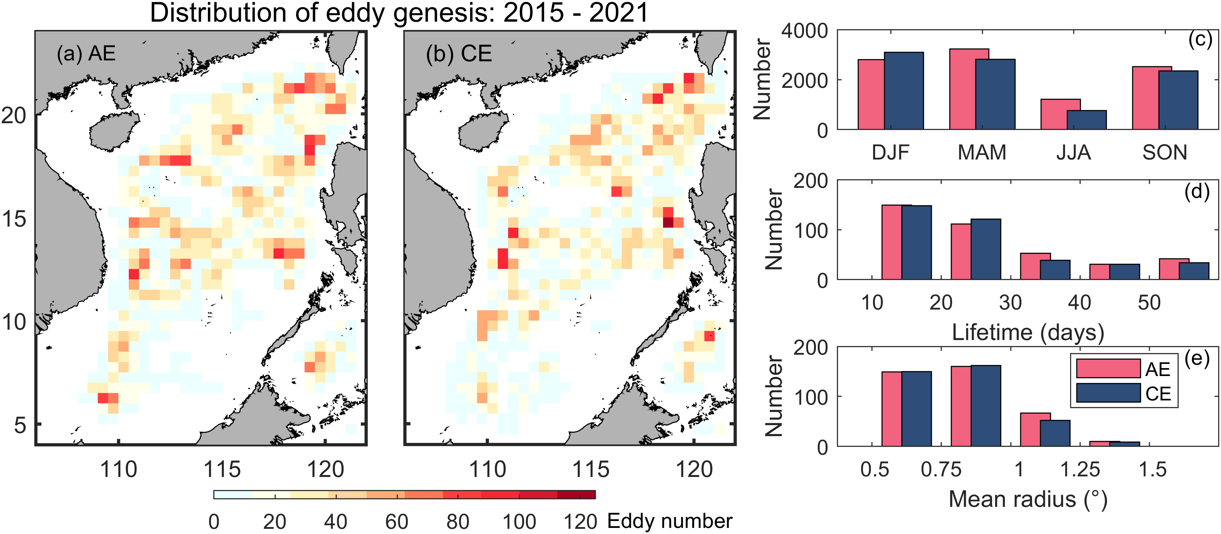
Figure 2 The distribution of (A) AEs and (red) (B) CEs (blue) in the SCS. The shaded area indicates the eddy number. The bar charts show the (C) seasonal distribution of eddies in the whole SCS (eddies are counted at each time step), distribution of (D) lifetime (unit: days) and (E) mean radius (unit: °) of eddies with full lifetime.

3) A total of 2317 salinity profiles of the South China Sea Physical Oceanic Dataset (SCSPOD) inside mesoscale eddies are chosen to verify the vertical salinity structure of AE and CE. SCSPOD is an SCS physical oceanography database combining observations with Argo, World Ocean Database (WOD), and mooring and ship-based data from the South China Sea Institute of Oceanology (Zeng et al., 2016).

2.2 Normalized eddy composite

Ocean eddies dominate the mesoscale process in the ocean (Melnichenko et al., 2021), so the normalized eddy composite method is frequently used in studies on eddy structure (Chelton et al., 2011; Hausmann and Czaja, 2012; Gaube et al., 2013). The SSS mesoscale variability accounts for 40% to 60% of the total SSS variability in the tropical Pacific (Delcroix et al., 2019). With the SSS dataset form SMAP, the eddies from SEIA will utilize boundary information to search for the simultaneous interior SSS region. For each gridded SSS anomaly (x, y) inside the eddy boundary, its position is normalized by the eddy radius (R) under eddy-centric coordinates as: $x_e=\frac{x}{L}, y_e=\frac{y}{L} (L=nR, n=1,2,3\dots )$. With such processing, each eddy will be converted into a circular structure spanning an n-standard radius. An averaging of many of these circular structures will yield eddy composites. Following this process, some unrealistic eddy-like structures with irregular boundaries can also be obtained, which do not truly represent the true eddy signal and may cause uncertainty in the overall eddy statistics. As suggested in Chen et al. (2021), oceanic eddies have a significant mean egg-like shape rather than a circle or ellipse considering the geophysical anisotropy in eddy properties. To eliminate unrealistic abnormal eddies in the detection process, some geometric-based constraints need to be incorporated in the algorithm, such as the eddy shape error (the ratio between the eddy boundary and the standard circle) and the eccentricity of the fitted ellipse of the eddy boundary (Kurian et al., 2011; Martínez-Moreno et al., 2019). In this work, only eddies with an eccentricity of less than 0.5 are considered to remove the singular boundary. As a result, a total of 3368 AEs and 1410 CEs are finalized and used to calculate the eddy composites for two eddy polarities in the SCS. Both climatological mean and seasonal eddy composites are provided in this study.

The empirical orthogonal function (EOF; Legendre and Legendre, 2012), also known as eigenvector analysis or principal component analysis (PCA), is a method for analyzing structural features in matrix data to extract the principal data features. It is now very widely used in geophysics and other disciplines. Here, EOF is performed to extract different salinity modes for eddy composites in the SCS. In this study, EOF analysis is adopted to decompose normalized circular eddy SSS structures in the SCS to evaluate the spatial patterns of eddy-induced SSS signals.

3 Results

3.1 Mean characteristics of eddy composites

From 2015 to 2021, a total of 3368 AEs and 1410 CEs are selected for normalization into eddy composites in the SCS (Figure 3). The area of the composites within a normalized radius of 1 indicates the actual eddy interior. Notably, there is a difference in the sampling of the two types of eddies, with more than twice the number of AEs than CEs (Figures 3A, B). However, the uncertainty in these salinity composites is small, with a standard deviation of approximately 0.02 psu (with a standard error on the order of $\frac{\mathrm{0.02 }}{\sqrt{\text{N}}}$ psu), which is consistent with the fact that the standard deviation of the intraseasonal variability in salinity is less than 0.02 psu (Yi et al., 2020). Thus, the difference in the mean salinity anomaly between AEs and CEs is significant. A subsampling test with randomly selecting the same amount of both types of eddies is performed, and a low sensitivity of the overall spatial patterns in eddy composites to subsampled eddy numbers is found.

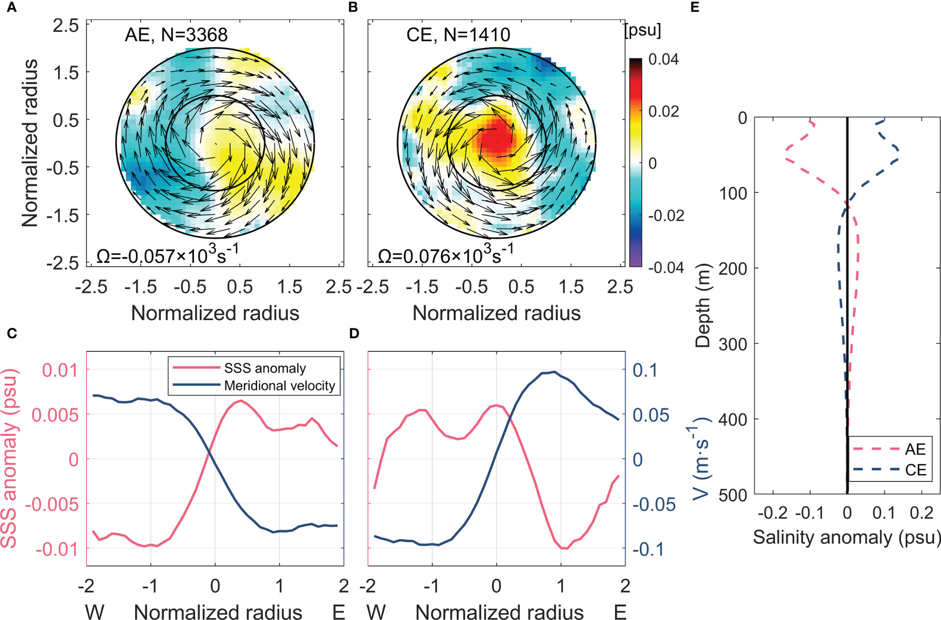
Figure 3 Normalized eddy salinity anomaly (shading, unit: psu) and current anomaly (vector, unit: m·s^-1) composites of (A) AE and (B) CE in the SCS. The number of eddy samples and eddy vorticity (Ω) are marked on each subgraph. The mean SSS anomaly (red line) and meridional velocity (blue line) of the AE and CE along the zonal section are shown in (C, D), respectively. (E) Mean salinity anomaly profiles of AE (dotted red line) and CE (blue line) in the SCS based on the SCSPOD dataset.

The eddy-induced composite-averaged salinity anomaly can be obtained from Figure 3, and the results show that the minimum and maximum AE-induced salinity anomalies may reach -0.10 and 0.05 psu, respectively, while the CE varies from -0.06 to 0.08 psu. The mean salinity anomalies in the eddies due to the presence of both types of eddies can be either positive or negative. However, the negative salinity anomaly related to the AE is more pronounced than that of the CE; instead, the CE induces a much stronger positive anomaly than does the AE. The AE salinity anomaly composite shows a clear dipole mode, with the eddy current anomaly being isotropic and rotating clockwise (Figure 3A). The salinity gradient is oriented from west to east, with low (~-0.01 psu) and high (~0.01 psu) salt cores located in the southwest and southeast of the eddy composite, respectively. In contrast to the AE, the CE composite presents a regular monopole structure, and the eddy current anomaly swirls in a counterclockwise direction. The CE composite basically exhibits a positive salinity anomaly except at the eastern edge, with the high-salinity (~0.03 psu) core slightly shifting to the northeast compared to the eddy center. The monopole pattern observed in the CE composite is mainly due to vertical eddy isothermal displacement and the dipole pattern is largely driven by lateral eddy advection of the background salinity gradient (Delcroix et al., 2019). Similarly, studies of eddy-induced chlorophyll anomalies also confirm the dominant role of background current fields on the distribution of eddy normalization (Gaube et al., 2013; He et al., 2016). In conclusion, the salinity anomaly signal within the CE composite is much more pronounced than that within the AE composite in terms of a multiyear climatology.

As suggested by Delcroix et al. (2019), the salinity anomaly pattern inside eddies is modulated by eddy-induced horizontal and vertical advection. To clarify these two advective effects, the mean SSS anomaly and meridional velocity (V) along the zonal section are depicted in Figures 3C, D. From west to the east of the AE composite, the SSS anomaly curve gradually increases from negative to positive values, reaching a peak at a 0.2 normalized radius. Generally, the meridional velocity decreases gradually, forming a quasi-symmetric structure around the eddy center together with the SSS anomaly curve. Such a dipole mode of the SSS anomaly of the eddy composite is out of phase with the meridional velocity, which will cause net salt transport over the eddy wavelength (Melnichenko et al., 2017) along the north−south direction. For the CE composite, the SSS anomaly along the zonal section is positive overall and peaks at a 0.1 normalized radius. Combining the east−west reversal meridional velocity, salinity advections in the western and eastern parts of the CE composite cancel each other, resulting in weaker net horizontal transport (approximately 30% smaller than that of AE), and the high-salinity anomalies concentrated near the eddy center, as shown in Figure 3B, may be induced by strong vertical advection (Delcroix et al., 2019).

The general perception of vertical motions in a mesoscale eddy is that the CE tends to upwell subsurface, salty seawater toward the surface, while the opposite is true for the AE. As shown in Figures 3A, B, the vorticity of the CE composite (0.076×10³ s^-1) has a larger magnitude than that of AE (-0.057×10³ s^-1). Based on the consideration of the vorticity, we may infer that the CE in the SCS is stronger than the AE in terms of vertical advection. To verify this hypothesis, mean eddy salinity anomaly profiles are calculated from the SCSPOD dataset and presented in Figure 3E, and the results are consistent with the results of He et al. (2018) that AE (CE) shows large salinity anomalies of approximately 0.14 psu (-0.16 psu) at the subsurface of approximately 50 m depth. The values of the AE salinity anomaly are negative in the upper layer (<120 m), with a peak at approximately 50 m and a value of -0.16 psu, and stable positive values remain in the lower layer (>120 m). The salinity anomaly profile of the CE has a quasi-symmetric trend with that of the AE.

The dominant effect of upwelling leads to a monopole mode in the CE composite. In contrast, the horizontal advection of the AE composite overrides the vertical advection. The most direct result is that the AE composite is not a monopole mode with a low salinity core, as we had previously thought. The difference in dipole/monopole patterns due to eddy polarity is not unique in the SCS, as the same phenomenon is also found in the central tropical Pacific region (Delcroix et al., 2019). This difference is presumably caused by the competition between vertical and horizontal advection.

3.2 Seasonal evolution of eddy composites

It has been shown that eddy activity in the SCS displays a strong seasonal signal (Figure 2C; Xing and Yang, 2021). Here, we evaluate the seasonal evolution of the eddy salinity anomaly composites in four seasons in the Northern Hemisphere, namely, boreal spring (December-January-February, DJF), summer (March-April-May, MAM), autumn (June-July-August, JJA) and winter (September-October-November, SON). The details are shown in Figure 4.

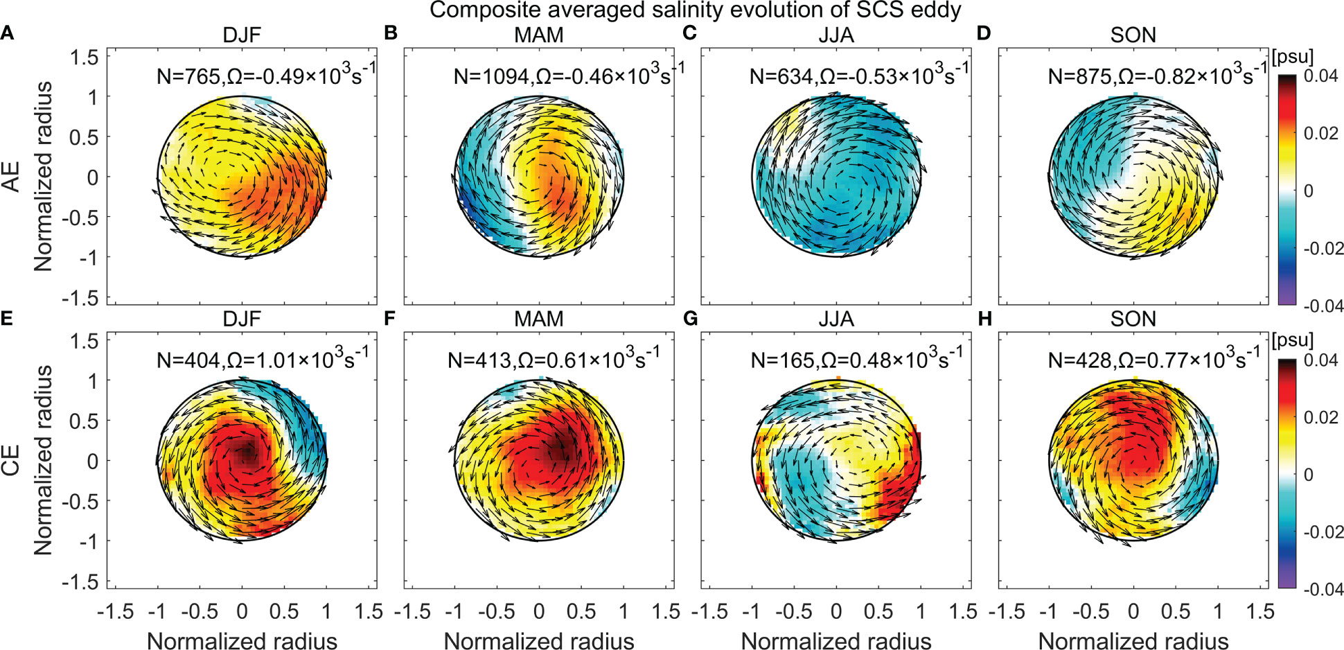
Figure 4 The seasonal evolution of the AE (A-D) and CE (E-H) eddy composites. The shading and vectors are the salinity anomaly (shading, unit: psu) and current anomaly (vector, unit: m·s^-1), respectively. The number of eddy samples and eddy vorticity (Ω) are marked on each subgraph.

During the spring, there is strong salinity advection in the eastern part of the AE composite compared with its western part (Figure 4A). By summertime, the salinity anomaly composite gradually develops into a significant dipole mode with low- and high-salinity cores in the west and east, respectively (Figure 4B). The SSS anomaly is not in phase with the meridional velocity, which will inevitably lead to large net transport as well. The AE composite is largely covered by the negative salinity anomalies during autumn, the season of the weakest eddy activity (N=634), except for the northwestern margin (Figure 4C). When winter arrives, the dipole mode reappears, but the salinity anomaly is slightly weaker in intensity than that in the summer, and the salinity gradient is in a northwest−southeast direction (Figure 4D). Overall, the east−southeast part of the AE salinity anomaly composite is dominated by positive salinity anomalies, accompanied by strong salinity advection, for most of the year, resulting in a prominent dipole mode (Figure 3A).

The situation for the CE differs from that of the AE, as the salinity anomaly composite exhibits obvious (quasi-) monopole modes in the spring, summer and winter (Figures 4E, F, H). It is conceivable that it will eventually behave as a monopole mode with a positive high-salinity core, as shown in Figure 3B. In autumn, the salinity anomalies appear more chaotic than those in other seasons (Figure 4G), but they still basically have a structure of low salinity in the west and high salinity in the east. In conclusion, the monopole mode of the CE composite initially forms in the winter, strengthens the following spring, and weakens and gradually shifts to the dipole mode the subsequent summer and autumn. The seasonal variation in the composite vorticity is consistent with the cycle of the salinity modes, as shown in Figure 4. The effect of vertical advection directly affects the maintenance of the monopole modes of the CE salinity anomaly composites. The larger amplitude in vorticity may be related to strengthened vertical advection, which in turn affects the seasonal mixed layer depth variation. Strong vorticity in the spring of the CE composite (Figure 4E) indicates prominent eddy-induced upwelling and thus shows a significant monopole mode. In investigating eddy effects on chlorophyll anomalies in the SCS, He et al. (2016) shows that the associated CHL anomalies are most apparent in winter and diminish in the following summer without polarity differences. The SSS anomaly patterns for both AE and CE are basically evident in winter and spring, while the diminishing time is delayed until autumn. Such seasonal variation in eddy-induced SSS anomalies generally corresponds to seasonally varying eddy activities in the SCS (Figure 2C). Active basin-scale eddy activities are more conducive to the formation of stronger eddies, thus maintaining more significant SSS anomaly patterns.

4 Discussion

It’s clearly indicated by Figure 3 that a dipole (monopole) pattern appears in the AE (CE) salinity anomaly composite in the long-term mean over the SCS basin. A seasonal partition further shows that the SSS anomaly patterns generally follow the trend of strengthening in winter and spring and weakening in autumn. To explore the possible mechanism of such characteristics, the EOF analysis is performed following Dufois et al. (2014), who successfully implemented such method to study the impact of eddies on surface chlorophyll in the Indian Ocean.

4.1 Multi-modes of eddy-induced salinity anomalies

The 7-year AE composites are decomposed by EOF analysis to obtain the spatial and temporal modes of eddy-induced salinity anomalies (Figure 5). The shading inside the composites indicates the spatial patterns of the salinity anomalies corresponding to EOF modes. The first three typical modes account for 79.7% of the variance, which basically represents the main characteristics of the original field. The first mode has an explained variance of up to 44.5% and exhibits a clear pattern of slightly off-center monopole (Figure 5A). The composite is covered with positive values. Combined with the time series of PC1 and its power spectrum, it can be seen that the variation in salinity anomalies of AE has no obvious dominant frequency but is influenced by (intra) seasonal and interannual variations (Figures 5B, C). The second mode exhibits a northwest to southeast dipole pattern with an explained variance of 22.2%, and its evolution is composed of variations at multiple time scales from seasons to years (Figures 5D–F). The third mode also exhibits a dipole pattern but is distributed in a northeast−southwest direction (not shown). For the of the CE composites, the decomposition results are similar to those of AE (Figures 5G–L). The first three typical modes exhibit the same spatial patterns of monopole, dipole and dipole, accounting for 68.2% of the variance. Its temporal variation may be determined by different processes from seasonal to interannual scales, even though there is no significantly dominant periodic variation found in the power spectral analysis (Figure 5I).

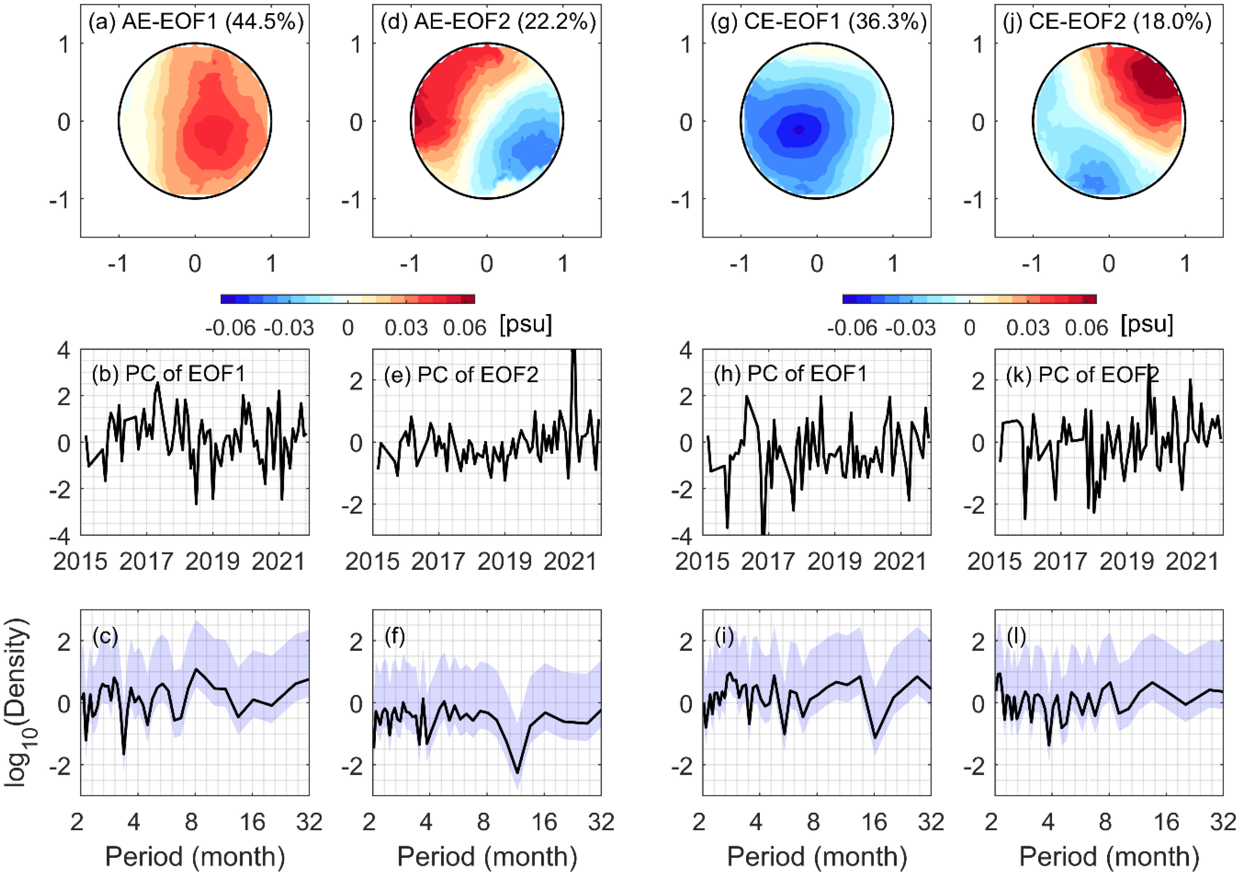
Figure 5 The (A) spatial pattern (unit: psu), (B) PC of EOF1, and (C) power spectrum of PC of the AE in the SCS. The shading indicates the salinity anomaly mode of the eddy composites and the purple area indicates the 95% confidence interval. Subgraphs (D-F) are for EOF2 of the AE in the SCS. Panels (G-L) are the same as (A-F) but for the first two modes of EOF of the CE in the SCS.

The results from EOF analysis show that the monopole pattern plays a dominant role in the salinity anomalies of the two types of eddies, followed by the dipole pattern. However, the composite analysis shows dipole and monopole patterns for AE and CE, respectively (Figure 2). This suggests that the climatological salinity anomalies of eddies are affected by the multi-patterns, but also by the magnitude of variability in each spatial pattern. Merging the first three EOF modes of the two types of eddies also yields the results of AE-dipole and CE-monopole, which are likely related to the modulation effect of advection. The upwelling inside the CE brings saline water from the lower layer and concentrates in the center, leading to a monopole mode, while the salinity reduction caused by the downwelling inside the AE is not strong enough and eventually results in a dipole mode by horizontal advection. This is consistent with the salinity situation reflected in Figure 3.

The power spectrum analysis of the PC time series cannot explain the seasonal variation in eddy-induced salinity anomalies well, since the intensity of the variations on multiple time scales is comparable. However, Dufois et al. (2014) demonstrated that the multipattern codominance of eddy normalization is partly related to seasonal adjustment of the mixed layer depth within eddies. Similarly, the weakening/strengthening in vertical advection due to seasonal adjustment of the mixed layer depth may also partly explain this seasonal variation in eddy-induced salinity anomalies.

4.2 Distribution of monopole and dipole modes

To clarify the distribution of the pattern characteristics of eddies, eddies in each 2.5° × 2.5° geographical subregion are normalized into composites for 7 years, and then the EOF analysis is applied individually. The first EOF mode in the normalized salinity anomaly is shown in Figure 6. For the AE, the average variance contribution of the first mode for the whole SCS is 46.6%, with the basin showing a monopole mode as a whole except for several subregions in the southwest and southeast (Figure 6A), where the shallower topography and islands make the eddies in these regions prone to odd boundaries and undersampling during the construction of the eddy composite. The poles of the monopole mode are slightly shifted from the center and exhibit quasi-isotropy. The monopole pattern of normalized CE composites predominantly appears in the west of the Luzon Strait and in the central part of the basin with a basin-mean variance contribution of 41.3%, and the subregions of the dipole pattern increase compared with that of AE. Different salinity anomaly patterns of eddies in each subregion are the result of modulation by multiscale processes.

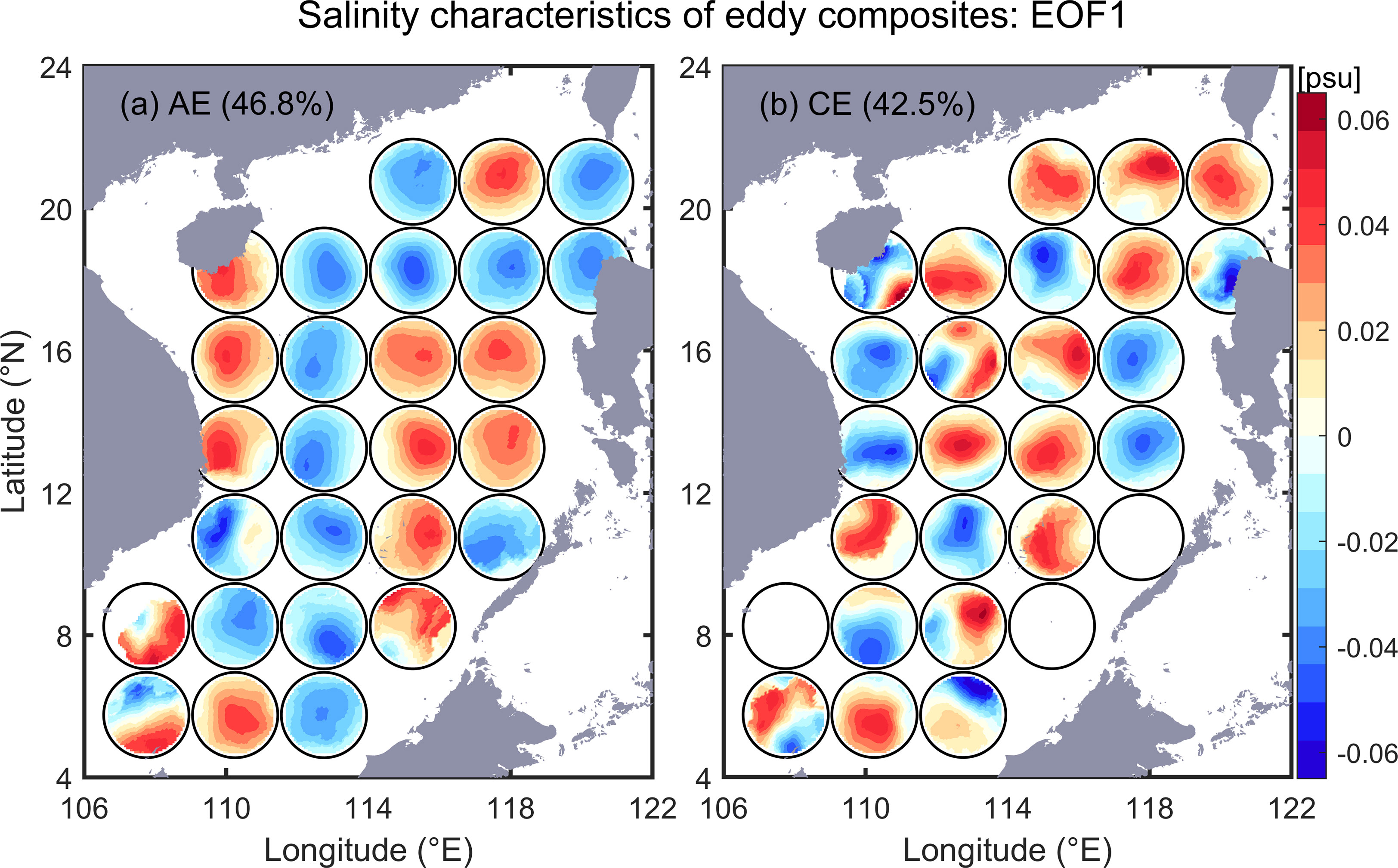
Figure 6 The first spatial pattern of the EOF of the (A) AE and (B) CE in the SCS. The shading indicates the salinity anomaly mode of the eddy composites.

The variance contribution of the second EOF modes for both types of eddies is approximately 30% (Figure 7). In EOF2, the AE and CE are consistent, with the whole basin being dominated by the dipole mode for the eddy composites. The directions of the salinity gradient inside the composites vary between subregions. For the formation of dipole modes, the initial SSS condition at the beginning of eddy formation and the background salinity gradient during subsequent evolution are very important to the salinity changes inside eddies. For both the AE and CE composites, the salinity gradient in the northern SCS is basically in a northeast−southwest direction, especially near the Luzon Strait. A possible explanation is that the Kuroshio intrusion brings much salty and warm Pacific water into the SCS via the Luzon Strait (Qu et al., 2004; Wang et al., 2020). This salt water moves along the northern slope of the basin, extending as far as the southeastern part of Hainan Island (Wang et al., 2015; Yi et al., 2020). Eddies can mix this part of the saltwater in the upper layer while moving northwestward, which has been confirmed as a key dynamic player in introducing and redistributing this Pacific water mass into the SCS (Yang et al., 2021).

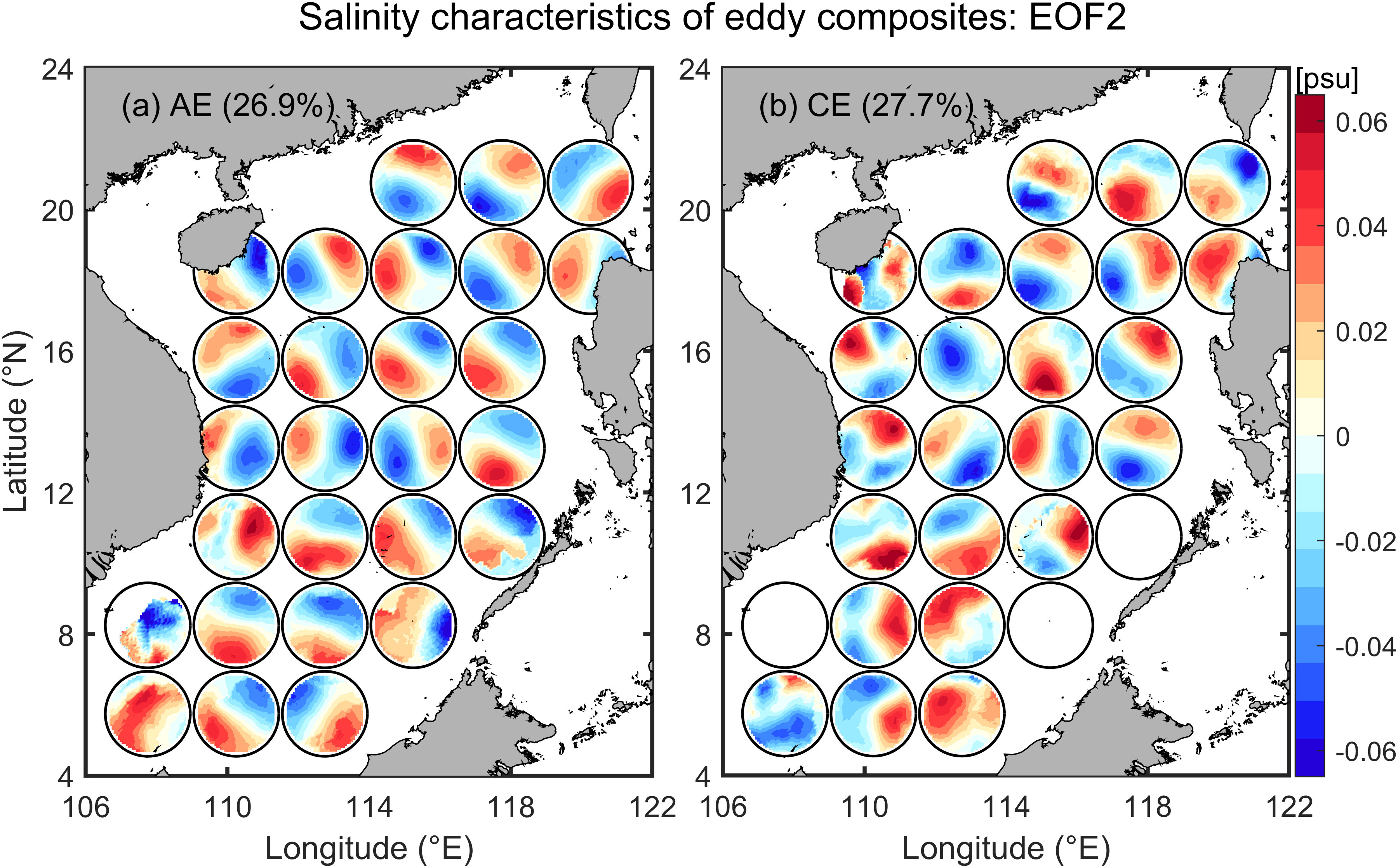
Figure 7 Similar to Figure 4 but for the second EOF mode of the (A) AE and (B) CE in the SCS.

The first two EOF modes explain more than 70% of the spatial variability in the eddy salinity anomaly, revealing that the SCS eddy is dominated by monopoles (EOF1) and supplemented by dipoles (EOF2). The interplay between relatively saline and freshwater in these monopole and dipole modes across the whole SCS basin gives rise to net salinity structures for AE and CE, as shown in Figure 3. The EOF analysis highlights the complexity of the spatial patterns of eddy-induced SSS anomalies in the SCS. The dipole (monopole) pattern in the first (second) mode may infer the role of horizontal (vertical) advection in driving the eddy-induced SSS anomalies. The complete mechanisms that are responsible for these spatial patterns need to be explored in the future studies based on model simulations.

5 Summary

Using SMAP satellite data, this study analyses the characteristics of the SSS anomaly associated with mesoscale eddies in the SCS. A total of 3368 AEs and 1410 CEs are detected and used for normalization into eddy composites from 2015 to 2021. The eddy-induced composite-averaged salinity anomalies of both types of eddies can be negative or positive, but the CE tends to have increased salinity overall, while the opposite is true for the AE. Moreover, the AE and CE eddy salinity anomaly composites feature dipole and monopole patterns, respectively. This leads to the SSS anomaly and meridional velocity being out of phase along the zonal section of the AE, causing net salt transport.

Furthermore, the climatological mean and seasonal characteristics of the salinity anomaly changes in eddies are examined under the long-term basin mean. The seasonal characteristics of the eddy salinity anomaly composites exhibit differences in eddy polarity. Dominated by horizontal advection, the AE composite exhibits a clear dipole mode, especially in boreal summer and winter, and strong positive salinity advection in the east−southeast part. The salinity changes inside the CE are basically controlled by vertical advection. From one winter to the next, the monopole mode of the CE composite experiences a whole cycle of formation, strengthening and weakening. The dominant advection process directly affects the salinity anomaly mode of the eddies.

By applying a spatiotemporal decomposition on eddy composites, for both AE and CE, the first three modes account for the vast majority of eddy-induced salinity anomaly variability, and the monopole pattern is dominant, followed by the dipole pattern. The eddy-induced salinity change is the result of the modulation of seasonal and (intra) annual processes, and the proportion of each is comparable. The spatial characteristics of the eddy-induced salinity anomaly in each 2.5°×2.5° geographical subregion further confirmed that the salinity anomaly distribution within eddies in the SCS is largely related to a monopole and a dipole spatial mode. The first two EOF patterns account for more than 70% of the spatial variability. The results show that the salinity anomaly composites of both types of eddies in the SCS are monopole-dominated and dipole-supplemented.

This work systematically investigates eddy-induced salinity changes with mesoscale-permitting satellite observations of the ocean surface salinity and geostrophic current in the SCS for the first time, along with its seasonal evolution and different spatiotemporal modes. Previous studies on eddy-induced features in the SCS were generally short in duration and used time series data from a limited spatial domain. The eddy composite and its different modes found in this work will provide an observational-based metric for model simulations. Previous studies have illustrated that background fields such as wind and current fields will have a significant effect on the eddy composite analysis (Frenger et al., 2013; Gaube et al., 2013; He et al., 2016). A complete mechanism for driving the observed dipole and monopole features in the eddy composite needs further investigation with numerical simulations in the near future.

Data availability statement

Publicly available datasets were analyzed in this study. These data can be found here: AVISO dataset distributed by Copernicus Marine Service (http://marine.copernicus.eu), the SEIA dataset can be obtained from the Science Data Bank (https://www.scidb.cn/en/s/Jbemmi) and the SMAP dataset from NASA (https://podaac-opendap.jpl.nasa.gov/opendap/allData/smap/L3/RSS/V4/8day_running/SCI/).

Author contributions

YY established the overarching research goals and aims, programmed the codes, and wrote the initial draft. YG assisted with the analysis of the results and revised the draft. LZ and QW verified the research protocol and supervised the planning and execution of research activities. All authors contributed to the article and approved the submitted version.

Funding

This research was supported by the National Natural Science Foundation of China (42076209), the Major State Research Development Program of China (2022YFC3103402), the Rising Star Foundation of the South China Sea Institute of Oceanology (NHXX2019WL0101) and the Science and Technology Planning Project of Guangzhou City, China (202102080363). YG is supported by Yale Center for Natural Carbon Capture.

Conflict of interest

The authors declare that the research was conducted in the absence of any commercial or financial relationships that could be construed as a potential conflict of interest.

Publisher’s note

All claims expressed in this article are solely those of the authors and do not necessarily represent those of their affiliated organizations, or those of the publisher, the editors and the reviewers. Any product that may be evaluated in this article, or claim that may be made by its manufacturer, is not guaranteed or endorsed by the publisher.

References

Boutin J., Chao Y., Asher W. E., Delcroix T., Drucker R., Drushka K., et al. (2016). SATELLITE AND IN SITU SALINITY understanding near-surface stratification and subfootprint variability. Bull. Am. Meteorol. Soc. 97 (8), 1391–139+. doi: 10.1175/bams-d-15-00032.1
Chelton D. B., Gaube P., Schlax M. G., Early J. J., Samelson R. M. (2011). The influence of nonlinear mesoscale eddies on near-surface oceanic chlorophyll. Science 334 (6054), 328–332. doi: 10.1126/science.1208897
Chen G., Gan J., Xie Q., Chu X., Wang D., Hou Y. (2012). Eddy heat and salt transports in the south China Sea and their seasonal modulations. J. Geophys. Res. 117, C05021. doi: 10.1029/2011JC007724
Chen G. X., Hou Y. J., Chu X. Q. (2011). Mesoscale eddies in the south China Sea: Mean properties, spatiotemporal variability, and impact on thermohaline structure. J. Geophys. Research-Oceans 116, C06018. doi: 10.1029/2010jc006716
Chen G., Yang J., Han G. (2021). Eddy morphology: Egg-like shape, overall spinning, and oceanographic implications. Remote Sens. Environ. 257, 112348. doi: 10.1016/j.rse.2021.112348
Delcroix T., Chaigneau A., Soviadan D., Boutin J., Pegliasco C. (2019). Eddy-induced salinity changes in the tropical pacific. J. Geophys. Research-Oceans 124 (1), 374–389. doi: 10.1029/2018jc014394
Delcroix T., McPhaden M. J., Dessier A., Gouriou Y. (2005). Time and space scales for sea surface salinity in the tropical oceans. Deep-Sea Res. Part I-Oceanogr. Res. Pap. 52 (5), 787–813. doi: 10.1016/j.dsr.2004.11.012
Ding R., Xuan J., Tao Z., Zhou L., Zhou F., Meng Q., et al. (2021). Eddy-induced heat transport in the south China Sea. J. Phys. Oceanogr. 51(7), 2329–2349. doi: 10.1175/JPO-D-20-0206.1
Dufois F., Hardman-Mountford N. J., Greenwood J., Richardson A. J., Feng M., Herbette S., et al. (2014). Impact of eddies on surface chlorophyll in the south Indian ocean. J. Geophys. Research-Oceans 119 (11), 8061–8077. doi: 10.1002/2014jc010164
Durack P. J. (2015). Ocean salinity and the global water cycle. Oceanography 28 (1), 20–31. doi: 10.5670/oceanog.2015.03
Durack P. J., Wijffels S. E., Matear R. J. (2012). Ocean salinities reveal strong global water cycle intensification during 1950 to 2000. Science 336 (6080), 455–458. doi: 10.1126/science.1212222
Frenger I., Gruber N., Knutti R., Muennich M. (2013). Imprint of southern ocean eddies on winds, clouds and rainfall. Nat. Geosci. 6 (8), 608–612. doi: 10.1038/ngeo1863
Gaube P., Chelton D. B., Strutton P. G., Behrenfeld M. J. (2013). Satellite observations of chlorophyll, phytoplankton biomass, and ekman pumping in nonlinear mesoscale eddies. J. Geophys. Research-Oceans 118 (12), 6349–6370. doi: 10.1002/2013jc009027
Gordon A. L., Huber B. A., Metzger E. J., Susanto R. D., Hurlburt H. E., Adi T. R. (2012). South China Sea throughflow impact on the Indonesian throughflow. Geophys. Res. Letters 39. doi: 10.1029/2012gl052021
Guo Y., Bishop S. P. (2022). Surface divergent eddy heat fluxes and their impacts on mixed layer eddy-mean flow interactions. J. Adv. Modeling Earth Syst. 14, e2021MS002863. doi: 10.1029/2021MS002863
Guo Y., Bishop S., Bryan F., Bachman S. (2022). A global diagnosis of eddy potential energy budget in an eddy-permitting ocean model. J. Phys. Oceanogr. 52 (8), 1731–1748. doi: 10.1175/jpo-d-22-0029.1
Hausmann U., Czaja A. (2012). The observed signature of mesoscale eddies in sea surface temperature and the associated heat transport. Deep-Sea Res. Part I-Oceanogr. Res. Pap. 70 (none), 60–72. doi: 10.1016/j.dsr.2012.08.005
He Q. Y., Zhan H. G., Cai S. Q., He Y. H., Huang G. L., Zhan W. K. (2018). A new assessment of mesoscale eddies in the south China Sea: Surface features, three-dimensional structures, and thermohaline transports. J. Geophys. Research-Oceans 123 (7), 4906–4929. doi: 10.1029/2018jc014054
He Q., Zhan H., Cai S., Li Z. (2016). Eddy effects on surface chlorophyll in the northern south China Sea: Mechanism investigation and temporal variability analysis. Deep-Sea Res. Part I-Oceanogr. Res. Pap. 112, 25–36. doi: 10.1016/j.dsr.2016.03.004
He Q., Zhan H., Xu J., Cai S., Zhan W., Zhou L., et al. (2019). Eddy-induced chlorophyll anomalies in the Western south China Sea. J. Geophys. Research-Oceans 124 (12), 9487–9506. doi: 10.1029/2019jc015371
Isern-Fontanet J., Olmedo E., Turiel A., Ballabrera-Poy J., Garcia-Ladona E. (2016). Retrieval of eddy dynamics from SMOS sea surface salinity measurements in the Algerian basin (Mediterranean Sea). Geophys. Res. Lett. 43 (12), 6427–6434. doi: 10.1002/2016gl069595
Jia Y. L., Liu Q. Y. (2004). Eddy shedding from the kuroshio bend at Luzon strait. J. Oceanogr. 60 (6), 1063–1069. doi: 10.1007/s10872-005-0014-6
Kerr Y. H., Waldteufel P., Wigneron J.-P., Delwart S., Cabot F., Boutin J., et al. (2010). The SMOS mission: New tool for monitoring key elements of the global water cycle. Proc. IEEE 98 (5), 666–687. doi: 10.1109/jproc.2010.2043032
Kurian J., Colas F., Capet X., McWilliams J. C., Chelton D. (2011). Eddy properties in the California current system. J. Geophys. Res. 116, C08027. doi: 10.1029/2010JC006895
Martínez-Moreno J., Hogg A. M., Kiss A. E., Constantinou N. C., Morrison A. K. (2019). Kinetic energy of eddy-like features from Sea surface altimetry. J. Adv. Modeling Earth Syst. 11, 3090–3105. doi: 10.1029/2019MS001769
Melnichenko O., Amores A., Maximenko N., Hacker P., Potemra J. (2017). Signature of mesoscale eddies in satellite sea surface salinity data. J. Geophys. Research-Oceans 122 (2), 1416–1424. doi: 10.1002/2016jc012420
Melnichenko O., Hacker P., Muller V. (2021). Observations of mesoscale eddies in satellite SSS and inferred eddy salt transport. Remote Sens. 13 (2), 315. doi: 10.3390/rs13020315
Qu T. D., Du Y., Sasaki H. (2006). South China Sea throughflow: A heat and freshwater conveyor. Geophys. Res. Lett. 33 (23), L23617. doi: 10.1029/2006gl028350
Qu T. D., Kim Y. Y., Yaremchuk M., Tozuka T., Ishida A., Yamagata T. (2004). Can Luzon strait transport play a role in conveying the impact of ENSO to the south China Sea? J. Climate 17 (18), 3644–3657. doi: 10.1175/1520-0442(2004)017<3644:Clstpa>2.0.Co;2
Storch J. S., Eden C., Fast I., Haak H., Hernandez-Deckers D., Maier-Reimer E., et al. (2012). An estimate of Lorenz energy cycle for the world ocean based on the 1/10° STORM/NCEP simulation. J. Phys. Oceanogr. 42, 2185–2205. doi: 10.1175/JPO-D-12-079.1
Sun W., Dong C., Tan W., Liu Y., He Y., Wang J. (2018). Vertical structure anomalies of oceanic eddies and eddy-induced transports in the south China Sea. Remote Sens. 10, 795. doi: 10.3390/rs10050795
Umbert M., Guimbard S., Lagerloef G., Thompson L., Portabella M., Ballabrera-Poy J., et al. (2015). Detecting the surface salinity signature of gulf stream cold-core rings in aquarius synergistic products. J. Geophys. Research-Oceans 120 (2), 859–874. doi: 10.1002/2014jc010466
Wang G., Su J., Chu P. C. (2003). Mesoscale eddies in the south China Sea observed with altimeter data. Geophys. Res. Lett. 30 (21), 6–1. doi: 10.1029/2003GL018532
Wang Q., Zeng L., Chen J., He Y., Zhou W., Wang D. (2020). The linkage of kuroshio intrusion and mesoscale eddy variability in the northern south China Sea: Subsurface speed maximum. Geophys. Res. Lett. 47 (11), e2020GL087034. doi: 10.1029/2020gl087034
Wang A., Zhuang W., Qi Y. (2015). Correlation between subsurface high-salinity water in the northern south China Sea and the north equatorial current-kuroshio circulation system from HYCOM simulations. Ocean Sci. 11, 305–312. doi: 10.5194/os-11-305-2015
Xing T., Yang Y. (2021). Three mesoscale eddy detection and tracking methods: Assessment for the South China Sea. J Atmos Ocean Technol. 38 (2). doi: 10.1175/JTECH-D-20-0020.1
Xiu P., Chai F., Shi L., Xue H. J., Chao Y. (2010). A census of eddy activities in the south China Sea during 1993-2007. J. Geophys. Research-Oceans 115, C03012. doi: 10.1029/2009jc005657
Yang Y., Wang D., Wang Q., Zeng L., Xing T., He Y., et al. (2019). Eddy-induced transport of saline kuroshio water into the northern south China Sea. J. Geophys. Research-Oceans 124 (9), 6673–6687. doi: 10.1029/2018jc014847
Yang Y., Zeng L., Wang Q. (2021). How much heat and salt are transported into the south China Sea by mesoscale eddies? Earths Future 9 (7), e2020EF001857. doi: 10.1029/2020ef001857
Yang Y., Zeng L., Wang Q. (2023). SEIA: A scale-selective eddy identification algorithm for the global ocean. Sci. Data (under review).
Yi D. L., Melnichenko O., Hacker P., Potemra J. (2020). Remote sensing of Sea surface salinity variability in the south China Sea. J. Geophys. Res.: Oceans 125 (12), e2020JC016827. doi: 10.1029/2020JC016827
Zeng L. L., Liu W. T., Xue H. J., Xiu P., Wang D. X. (2014). Freshening in the south China Sea during 2012 revealed by aquarius and in situ data. J. Geophys. Research-Oceans 119 (12), 8296–8314. doi: 10.1002/2014jc010108
Zeng L., Schmitt R. W., Li L., Wang Q., Wang D. (2019). Forecast of summer precipitation in the Yangtze river valley based on south China Sea springtime sea surface salinity. Climate Dynam. 53 (9-10), 5495–5509. doi: 10.1007/s00382-019-04878-y
Zeng L. L., Wang D. X., Chen J., Wang W. Q., Chen R. Y. (2016). SCSPOD14, a south China Sea physical oceanographic dataset derived from in situ measurements during 1919-2014. Sci. Data 3, 160029. doi: 10.1038/sdata.2016.29
Keywords: mesoscale eddy, sea surface salinity, South China Sea, eddy composite, dipole and monopole
Citation: Yang Y, Guo Y, Zeng L and Wang Q (2023) Eddy-induced sea surface salinity changes in the South China Sea. Front. Mar. Sci. 10:1113752. doi: 10.3389/fmars.2023.1113752
Received: 01 December 2022; Accepted: 17 February 2023;
Published: 07 March 2023.
Edited by:
Zexun Wei, Ministry of Natural Resources, ChinaReviewed by:
Ge Chen, Ocean University of China, ChinaQingxuan Yang, Ocean University of China, China
Hailong Liu, Institute of Atmospheric Physics (CAS), China
Copyright © 2023 Yang, Guo, Zeng and Wang. This is an open-access article distributed under the terms of the Creative Commons Attribution License (CC BY). The use, distribution or reproduction in other forums is permitted, provided the original author(s) and the copyright owner(s) are credited and that the original publication in this journal is cited, in accordance with accepted academic practice. No use, distribution or reproduction is permitted which does not comply with these terms.
*Correspondence: Lili Zeng, zenglili@scsio.ac.cn; Yikai Yang, yangyikai@scsio.ac.cn`