Investigating how river flow regimes impact on river delta salinization through idealized modeling

1 Introduction

Rising sea level and decreasing streamflow threaten water resourcing and freshwater availability by causing an upstream intrusion of the saltwater zone (Gornitz, 1991; Bhuiyan and Dutta, 2012; Hong and Shen, 2012; Hong et al., 2020; Bricheno et al., 2021). Saltwater intrusion (SI) is much exacerbated in low lying areas such as deltas (Zhou et al., 2017). SI is a serious problem that affects households, agriculture, irrigation and industry (Allison, 1964; Smedema and Shiati, 2002; Zhang et al., 2011) because rivers and aquifers contaminated by high salinity decrease freshwater storage and water quality (Gornitz, 1991). In addition, SI reduces soil fertility resulting in low crops yield (Bhuiyan and Dutta, 2012), threatens vegetation and freshwater species with limited salinity tolerance (Visser et al., 2012; White et al., 2019), increases plants mortality (Kaplan et al., 2010; Bhuiyan and Dutta, 2012) and affects human health (Sarwar, 2005; Rahman et al., 2019).

Many deltas face already the consequences of saltwater intrusion including the Mekong in Vietnam (Nguyen and Savenije, 2006; Trieu and Phong, 2015; Eslami et al., 2019) the Ganges-Brahmaputra in Bangladesh (Nobi and Das Gupta, 1997; Bhuiyan and Dutta, 2012; Rahman, 2015; Yang et al., 2015; Bricheno et al., 2016; Sherin, 2020; Bricheno et al., 2021), the Mississippi in the Gulf of Mexico (Holm and Sasser, 2001; Day et al., 2005; Das et al., 2012), the Yangtze in China (Chen et al., 2001; Hu and Ding, 2009; Dai et al., 2011; Qiu and Zhu, 2015), the Pearl River (Liu et al., 2019; Hong et al., 2020) and the Nile Delta (Frihy, 2003). Unfortunately, limitations in water supply come along with an increase in water demand because of population growth, economic development, and land use changes (Phan et al., 2018).

Sustainable water management and enhanced water conservation practices are necessary for the available water supply to meet with the future demand (Dawadi and Ahmad, 2013). These practices often rely on the assumption that salt intrusion reduces as river discharge increases (Garvine et al., 1992; Gong and Shen, 2011). In the absence of tides or other driving mechanisms (i.e., atmospheric or oceanic forcing) the river discharge dominates the salinity distribution (Valle-Levinson and Wilson, 1994; Wong, 1995; Monismith et al., 2002). During the 20th century, water management relied on technical and engineering solutions (Ha et al., 2018). The so called ‘hard-path’ approach consisted of dams, aqueducts, pipelines and complex treatment plants (Gleick, 2003). However, this type of solutions often comes with a cost. For example, tens of millions of people have been displaced by their homes due to water related projects (Adams, 2000) while the freshwater flows reaching many deltas are not adequate anymore and this has several consequences for the local environment and population (Gleick, 2003). Recently, the need for more adaptive management to sustain freshwater resources has been identified (Ha et al., 2018; Zevenbergen et al., 2018). A ‘soft-path’ approach for water is now promoted that would include regulatory policies for better use of existing water resources than seeking for additional ones (Gleick, 2002). In this context, an efficient water usage is preferred with equitable distribution and sustainable system operation over time while local communities should be also included in water management decisions (Gleick, 2002; Gleick, 2003). Within this concept, the problem of saltwater intrusion in deltas could probably be mitigated by an efficient water management of a catchment’s freshwater availability instead of resorting to technical solutions. This could be achieved for example by storing a certain amount of water that is available during a wet season and supply it during the next dry season when the demand for freshwater is higher. Coastal reservoirs -water storage structures constructed at a river estuary or other coastal area to store fresh water and control water resources- have already been constructed in China, South Korea, Hong Kong and Singapore (Yuan and Wu, 2020; Tabarestani and Fouladfar, 2021). These structures are constructed near the coast, in natural river basins and have a smaller environmental footprint compared to other technical solutions (Sitharam et al., 2020). An additional advantage is that they could be used for the generation of tidal renewable energy assisting further into the development of sustainable and environmentally friendly infrastructure (Sitharam et al., 2020). Independent of a hard or soft path, the main management strategy is to affect river discharge, which is likely to cause changes to the annual hydrograph. Such changes are also expected to occur as a consequence of natural climate variability and anthropogenic climate change (Deser et al., 2012; Zhang and Delworth, 2018). Possible effects to deltas’ salinity distribution from these changes need to be assessed. Even though salinity response to changes in river discharges has been studied extensively in estuaries (Garvine et al., 1992; Wong, 1995; Uncles and Stephens, 1996; MacCready, 1999; Chen et al., 2000; Monismith et al., 2002; Bowen, 2003; Banas et al., 2004; Chen, 2004; Hetland and Geyer, 2004; Brockway et al., 2006; Liu et al., 2007; Lerczak et al., 2009; Gong and Shen, 2011; Wei et al., 2016) it is still unclear if and how this changes in the presence of a channelized network.

The present study investigates the effect of various annual flow distributions of equal water volume on the salt intrusion. The paper tries to answer questions such as: 1) how salinity responds to flow changes, 2) what is the impact on salinity from changes in hydrographs' shape 3) which flow distribution cause the maximum increase of mixing in the delta and 4) which flow regime ensures fresher water conditions for the longest period and to what extent.

The answer to the last question derives from measuring flushing and residence times that are useful tools to assess the efficacy and adequacy of a certain flow distribution for averting the salt intrusion (Choi and Lee, 2004; Sámano et al., 2012). Flushing time (FT) is defined as the time required for the cumulative freshwater inflow to equal the amount of freshwater originally present in the region (Dyer, 1973; Sheldon and Alber, 2002). The simplest and most common method for the FT calculation is the freshwater fraction in which the freshwater volume is divided by the freshwater input (Dyer, 1973; Fischer et al., 1979; Williams, 1986). A difficulty on the determination of the freshwater volume and input arises in the case of unsteady flow and tidal conditions. Many researchers implemented the method by taking averages over a certain period (Pilson, 1985; Christian et al., 1991; Balls, 1994; Lebo et al., 1994; Eyre and Twigg, 1997; Alber and Sheldon, 1999; Hagy, et al., 2000; Huang and Spaulding, 2002; Sheldon and Alber, 2002; Huang, 2007). Alber and Sheldon (1999) proposed a specific technique to determine the appropriate averaging period of the river discharge by assuming that this should be equal or very close to the flushing time itself. They tested their method in Georgia Estuaries. Whereas the FT is a unique value representative of an entire water body, the residence time (RT) is a measure of spatial variation (Choi and Lee, 2004; Sámano et al., 2012). It is defined as the remaining time that a particle will spend in a defined region after first arriving at some starting location (Zimmerman, 1976; Sheldon and Alber, 2002). Therefore, the RT is applied within a restricted geographical area such as an estuary, a water basin or a box model (Hagy et al., 2000; Sheldon and Alber, 2022; Sámano et al., 2012).

In this study, the concept of RT is adapted to measure the time that the water remains fresh within the delta. This requires a definition of what exactly fresh water is which is usually case dependent. There are salinity standards for execution of certain activities and survival of vegetation species and aquatic life. For instance, salinity in the water has to be at least less than 1 PSU for it to be potable (Ahmed and Rahman (2000); Sarwar (2005); Dasgupta et al. (2015)) and crop yields can be severely affected if salinity is more than 4 PSU (Clarke et al., 2015). Some aquatic organisms (e.g. phytoplankton, larvae fish, shrimps, smelt etc.) and vegetation (e.g. Sagittaria Latifolia, Sagittaria Lancifolia, phragmites australis) species do not survive in environments with more than 2 PSU salinity (Jassby et al., 1995; Visser et al., 2012; Hutton et al., 2016; White et al., 2019; Wang et al., 2020). In particular, the location of the 2-PSU bottom isohaline has been found to have significant statistical relationships with many estuarine resources (e.g., phytoplankton, larvae fish, shrimps, smelt etc.) (Jassby et al., 1995; Hutton et al., 2016). It is also a threshold for freshwater wetlands conversion to brackish marsh (Conner et al., 1997; Wang et al., 2020). Therefore, the location of 2 PSU isohaline has been established as a salt intrusion measure in many similar studies (Schubel, 1992; Monismith et al., 1996; Monismith et al., 2002; Herbold and Vendlinkski, 2012; Andrews et al., 2017). In this context, a freshwater RT in this study is determined to be the time that the salinity remains below 2 PSU.

For the purposes of this study, a 3D numerical model for an idealized delta configuration is built in Delft3D. Idealization is chosen with the consideration that idealized (or exploratory) models can offer simpler and better explanations of certain behaviors in systems involving many interacting processes (Murray, 2002). In this approach, some parameters are intentionally omitted (e.g., tides and/or waves) and only the core causal factors (e.g., river discharge) are retained (Weisberg, 2007). Idealized studies have the advantage of reducing the complexity that is found in real systems and provide a better physical insight on the effect of a certain variable in a physical phenomenon isolated from others. Therefore, the use of idealized models aims to reveal the direct impact of external forcing factors in a system’s variable separately for each one of them. In this paper, five simulations with different flow distributions are carried out. The implemented hydrographs follow typical distributions similar to some that can be often found in real deltas. The paper aspires to provide answers through the idealized modeling for a more sustainable use of freshwater resources in deltaic systems.

2 Methods

2.1 Model setup

Matsoukis et al. (2022) built a 3D model with an idealized delta configuration to investigate the impact of tidal level changes in a static delta’s salinity neglecting morphological changes. The same model is used in this paper. The model –that was built in Delft3D (Deltares, 2014)- uses a structured rectangular grid with dimensions of 20 km to 22 km. The grid resolution varies from 50 m to 200 m in the X direction and between 20 m and 100 m in the Y direction of a Cartesian co-ordinate system. The delta was built by implementing a high and constant river discharge of 3000 m³/s in an initially uniform bathymetry. The flow enters in the domain through an inlet of 1.3 km length and 380 m width. Erosion and sedimentation caused by the river discharge resulted in the delta bathymetry that can be seen in Figure 1F. The delta covers an area of 4.8 km x 8 km. A bed slope of 0.5⁰ has been imposed 10 km downstream of the river boundary so that the water depth reaches 30 m at the offshore boundary. The full model’s bathymetry can be seen in the Supplementary Material. To note that results analysis shown in this paper includes only the delta area as it is presented in Figure 1F and excludes the deeper offshore area outside of it as the focus is restricted only within the delta limits. The model’s bathymetry remains constant during the simulations and there is no sediment input. Bed level changes are not considered so that the impact of flow distributions on the salinity is isolated from any morphological effects. The vertical resolution consists of eight sigma layers. Higher numbers of vertical layers were considered too. However, it was found that the increase of vertical layers had only a quantitative and not qualitative impact on the results. The main conclusions for each paper's section remained unaffected, probably due to the relatively shallow water depths. Considering that this is an idealized study where the actual magnitude values are not so important, it was decided then to keep the vertical resolution equal to 8 layers to satisfy computational efficiency limitations for a full year study. The default Delft3D values for horizontal diffusion and viscosity are introduced in the model equal to 10 m²/s and 1 m²/s respectively that were found to be the optimum for model’s performance and stability. A relatively large diffusion coefficient is justified for large scale applications where estuarine physics apply. In addition, diffusion can vary a lot when seasonal flows for a one-year simulation period are implemented as they may cause substantial salinity changes in the vertical (Monismith et al., 1996). The vertical diffusion is fully modelled by the κ-ϵ turbulence closure model. A spatially constant Chezy coefficient (45 m^1/2/s^-1) is implemented to account for bed roughness in accordance with what has been used in other idealized delta studies with Delft3D (Edmonds and Sligerland, 2010; Leonardi et al., 2013; Caldwell and Edmonds, 2014; Burpee et al., 2015; Liu et al., 2020). A cyclic implicit numerical scheme is used, and the time step is 30 seconds being the optimum value for both model stability and computational time. Further details on the model’s parameters and the process of bathymetry development can be found in the Supplementary Material (S1).

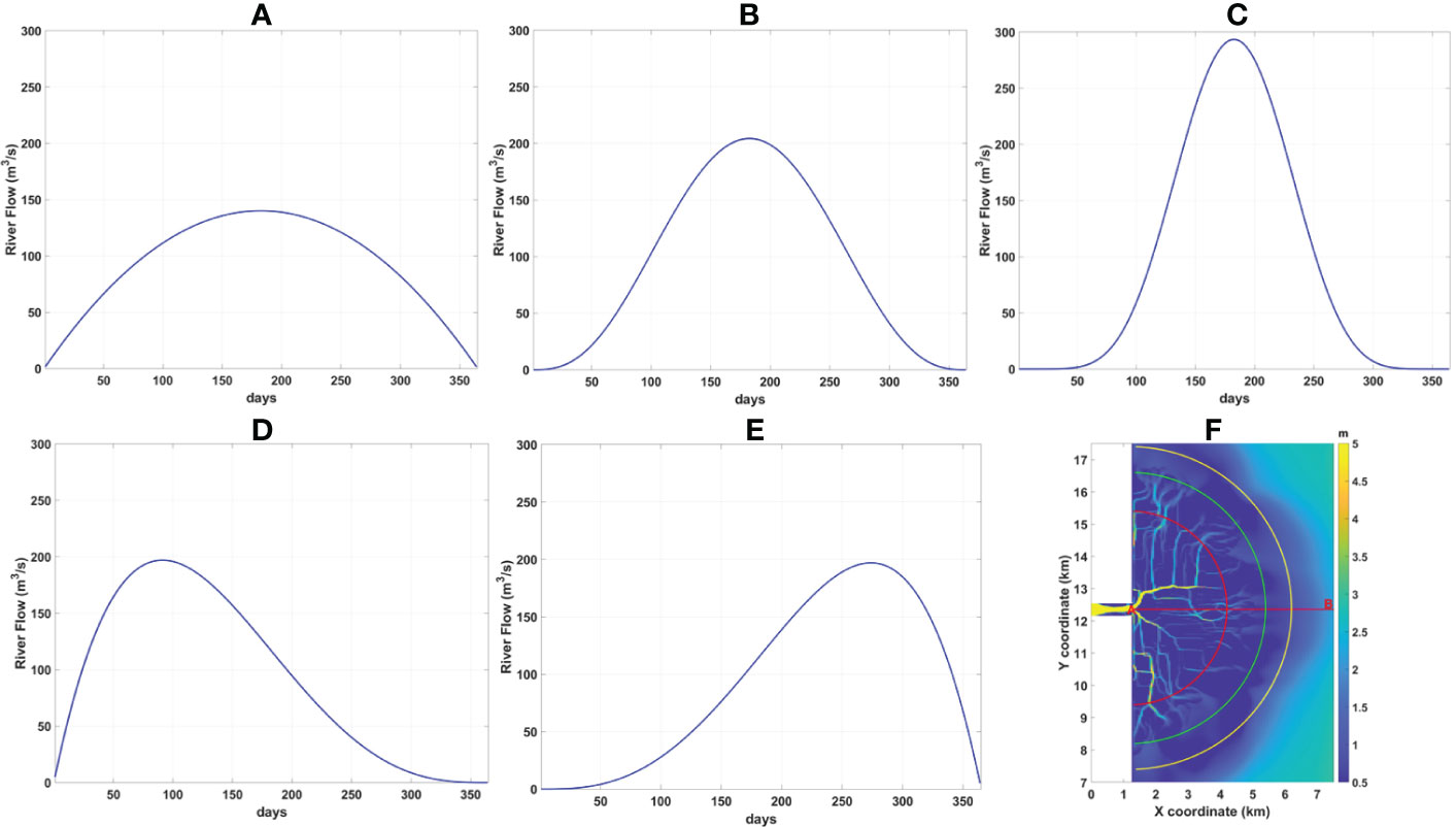
Figure 1 The hydrographs implemented in the model: (A) Platykurtic (B) Mesokurtic (C) Leptokurtic (D) Left Skewed and (E) Right Skewed flow distribution for one year. (F) The delta bathymetry. The red line AB measures the 6km distance from the river mouth (point A) corresponding to the length of the salt intrusion curve displayed in Figure 2B. The colored semicircles with their centre at point A and radius 3km (red), 4.2km (green) and 5km (yellow) visualize the cross sections over which salinity is averaged for the results analysis in sections 3.1, 3.2 and 3.4.

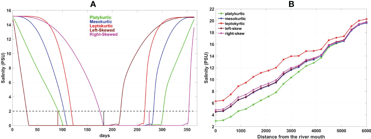
Figure 2 (A) Time series of the bottom salinity at the river mouth (point A in Figure 1F). Each colour represents results for a simulation with a different hydrograph. The dashed black line draws the 2 PSU threshold. The short brown, magenta and black vertical lines indicate the time moment of the peak flow on the horizontal axis for the left skewed, right skewed and symmetric distributions equal to 91, 274 and 183 days respectively. (B) Annual averages of the mean over depth salinity when averaged radially every 300 m along a distance of 6 km from the river mouth.

2.2 Hydrodynamic forcing

The model is forced with an annual river flow distribution. Five simulations are setup with hydrographs of equal water volume but different shape each time. This is achieved by implementing the Beta (B) function to an original hydrograph and obtain five beta distributions. The Po delta flow distribution for 2009 (Montanari, 2012) is used as the original hydrograph to build the five idealized ones. The use of the 2009 Po delta hydrograph does not imply any resemblance with the idealized delta and is chosen merely as a guide. To build a beta distribution the following equation is used (Yue et al., 2002):

Where B is the probability density function, x is the probability of occurrence of each daily flow taken equal to 1/365 for an annual distribution. The shape parameters α and β determine the shape of the hydrograph. The normalized probability distribution is then converted to a flow distribution by multiplying by the annual water volume of the original hydrograph (Po Delta in 2009). Consequently, the five idealized hydrographs contain the same water volume with the original one. However, the size of the idealized delta is much smaller than the Po delta and the implementation of the original flow range causes stability issues in the model. Therefore, the hydrographs are reduced by the river cross-sections’ ratio between the real (Po Delta) and the idealized delta. The produced hydrographs can be seen in panels a-e of Figure 1. Table 1 presents the basic statistic parameters for each beta distribution. Equal shape parameters result into symmetric hydrographs (Figures 1A-C) and the higher their value the higher the peak is. When α is smaller than β a left skewed hydrograph occurs (Figure 1D). The hydrograph exhibits right skewness when β is smaller than α (Figure 1E).

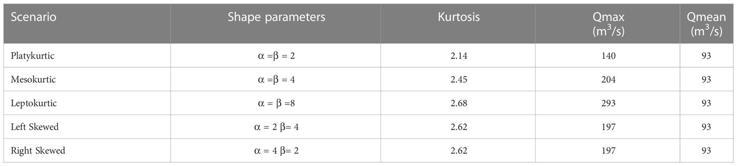
Table 1 Statistical parameters for each hydrograph type.

The five hydrographs in Figure 1 can be qualitatively classified based on their shape and the tails of each distribution as: 1) Platykurtic (light tails and low peak), 2) Mesokurtic (relatively light tails and medium peak), 3) Leptokurtic (heavy tails and high peak), 4) Left skewed (long tail on the right) and 5) Right skewed (long tail on the left). All of them correspond to seasonal regimes with a pronounced wet season (Hansford et al., 2020). The distinction between heavy and light tails in this paper is defined as follows: heavy tails indicate distributions with larger probability of getting an outlier (e.g., leptokurtic) and light tails indicate distributions that go to zero faster than the exponential distribution (e.g., platykurtic) (Bryson, 1974; Glen, 2016).

Small scale discharge events have been purposefully neglected in the five hydrographs that all have smooth shapes. The use of irregular shapes would add into complexity – in contrast to the benefits of a simplified and idealized approach- and would hinder the extraction of concrete conclusions on the effects of hydrographs shape. However, an indication of potential transient peaks effects and larger flow amplitudes can be given if comparing results between the three symmetric distributions.

Annual flow distributions with shapes close to the hydrographs of Figure 1 are recorded often in many real deltas. For example, left skewed hydrographs (Figure 1D) were reported in deltas located at the Gulf of Mexico including the Wax Lake Delta in the years between 2006 and 2010 (Shaw et al., 2013) and the Mississippi Delta between 1993 and 2012 (Kolker et al., 2018). Based on large data records from internet data bases and national agencies, Latrubesse et al. (2005) showed that the Mekong and the Ganges-Brahmaputra river catchments develop usually right skewed annual hydrographs (Figure 1E). The Yangtze delta sees its peak flow often in the middle of the year at some time during the wet season that occurs between May and September (Birkinshaw et al., 2017). Such flow distributions are similar to that of Figure 1C and have been reported in the years between 1996 and 2005 (Lai et al., 2014; Birkinshaw et al., 2017) in the Yangtze Delta. In addition, when Hansford et al. (2020) averaged daily flow data for one year between 1978-2009 in the Parana Delta (Argentina), they detected an annual flow hydrograph very similar to a platykurtic distribution (Figure 1A). Finally, mesokurtic hydrographs as the one in Figure 1B have been observed in the Colorado and Nile deltas. Averaged annual hydrographs for the 1950-1993 period in the Colorado (Pitlick and Cress, 2000) and flow distributions at several stations in the Nile (Eldardiry and Hossain, 2019) confirm this. The averaged over the years 1984-1996 annual hydrograph in the Niger Delta also exhibited a mesokurtic hydrograph shape (Lienou et al., 2010).

2.3 Boundary conditions

A zero-water level is implemented at the offshore boundary while the Riemann condition (in the form of a zero-velocity variant) applies in the lateral boundaries. Fresh water is assumed at the upstream river boundary and seawater salinity (30PSU) at the offshore and lateral boundaries. Special care was taken at the lateral (north and south) boundaries so that the freshwater plume is not clamped by the imposed seawater salinity but is allowed to spread radially with no boundary effects. This is possible to do in Delft3D by setting the horizontal diffusion equal to zero only at the two last grid lines along these two boundaries. In this way, the model is allowed to calculate its own salinities close to the boundaries unaffected of the imposed 30 PSU.

2.4 Initial conditions

A spin-up simulation precedes each time to get a dynamic equilibrium for salinity to be introduced as initial conditions. A uniform salinity equal to 30 PSU is implemented in the model except for the river upstream boundary where zero salinity is imposed. It is decided to spin-up the model with the initial flow of each hydrograph in Figure 1. These are very small but non-zero values and this reduces the time required to reach a dynamic equilibrium. This means that the simulations start in dry season (low flows) conditions. The river flow in the spin-up model is constant and the simulation is stopped after 30 days when steady state conditions are reached in all cases. The full model setup is summarized in Table 2.

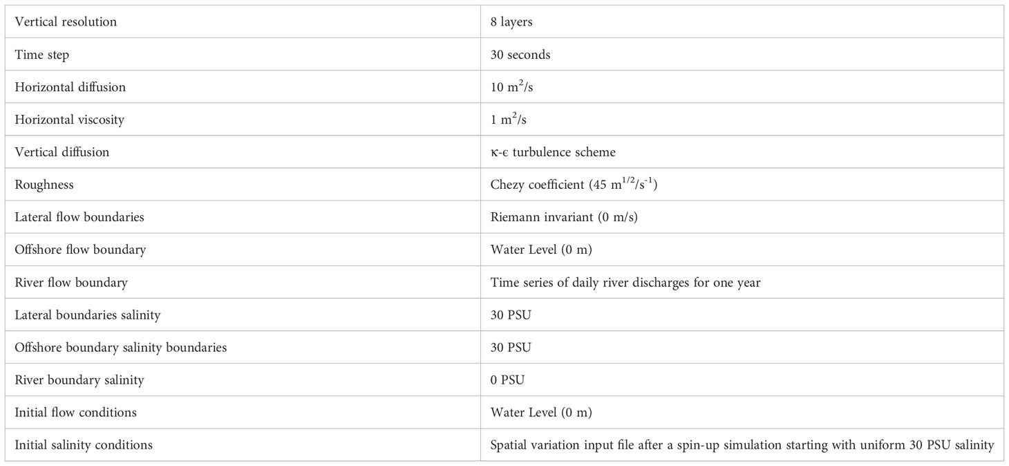
Table 2 Summary of the main model setup parameters.

2.5 Assumptions and limitations

The goal of the study is to assess the effects of flow regimes on the salinity distribution isolated from any other effects (i.e., tides and waves). Therefore, the delta’s idealized bathymetry has been developed after a morphological simulation where no tidal forcing is considered and subsequently no tides are included in the five simulations of different annual flow distributions. This decision is taken on the grounds that a different morphology would be required if tides were included as it is known that tides have a strong influence together with river discharges on deltas’ morphology depending on their range (Galloway, 1975). Even though this may compromise the applicability of the results, the present bathymetry retains many typical and common delta features such as the erosion in front of the river mouth and the downstream shallowing and widening of the channels (Hori and Saito, 2007; Lamb et al., 2012). In addition, the idealized delta exhibits bathymetric irregularities with deeper channels on the left of the delta apex (looking seaward) and shallower right of it. Due to the presence of such common and special features of deltas morphology, the model can capture bathymetric effects on the salinity horizontal and vertical distribution that would have not been uncovered if a more simplified bathymetry had been implemented. This is crucial because the role of bathymetry on salinity distribution is important as it has been identified in previous studies as well (Sridevi et al., 2015; Wei et al., 2017; Matsoukis et al., 2022). In addition, the world’s deltas are reported to be in a continuous state of transition regarding their dynamic morphological equilibrium due to natural climate change and human activities and thus such irregularities may not be uncommon (Hoitink et al., 2017).

Matsoukis et al. (2022) identified these irregularities as the cause of asymmetries in the salinity distribution between delta areas especially during low flow seasons. They then neglected Coriolis force on this basis to avoid an extra source of asymmetry in the model, something that is adopted in this work as well with the same justification. Nevertheless, this omission is not expected to have remarkable impact on the results in this specific case. Buoyant plumes may become geostrophic dominated only beyond the near-field region (Horner-Devine et al., 2015) where momentum balance is yet mainly dominated by barotropic and baroclinic pressure gradients, frictional stresses, and flow acceleration (McCabe et al., 2009). But specifically in deltas, freshwater plumes are formed at the channels outlets and interact with each other (Yuan et al., 2011; Horner-Devine et al., 2015) to form larger scale ones. This goes beyond the focus area in this study as depicted in Figure 1F where Coriolis force effects would be minimal. Likewise, wind forcing is usually considered of second order in the near-field region (Kakoulaki et al., 2014) although there are recent indications that plume dynamics may be more sensitive to winds than previously assumed (Kakoulaki et al., 2014; Kastner, 2018; Spicer et al., 2022). Despite this, the wind effects on the plume’s orientation, spreading, thickness and mixing and their subsequent impact on flushing, residence times and stratification have not been considered in this case. The reason is that the wind acts intermittently and in much smaller time scales compared to the annual flow distributions of the current setup and the direct effect of the latter would not be discernible.

The above simplifications would indicate that the applicability of this paper’s findings might be limited to river dominated deltas or at least deltas with little tidal influence and in medium latitudes. These may include for example deltas in the Gulf of Mexico (Mississippi, Atchafalaya and Wax Lake), Orinoco, the Danube, the Irrawaddy and the Po delta.

However, idealized modeling does not aim to provide specific answers and solutions directly interpretable to real systems. Real case models should be used for such purposes. The level of complexity in real systems is such that non-linear effects cannot always be captured by idealized models where several simplifications are considered. Nonetheless, the advantage of idealized models is that they are more oriented towards a ‘knowledge obtaining’ and fundamental physical analysis that results in more general and universal conclusions. In that sense, the present work’s conclusions can refer to a larger number of deltas than those mentioned in this section and with various hydrodynamic conditions.

2.6 Flushing time calculation

Flushing time (FT) is measured in section 3.6 for each flow regime. The river delta as depicted in Figure 1F is considered for the calculation which is executed based on the ‘freshwater fraction method’ given by the following equation (Dyer, 1973; Alber and Sheldon, 1999):

For a total number n of grid cells i, V_i and S_i are its volume and salinity respectively. S_SW is the sea water salinity (in this case equal to 30 PSU) and Q_F an averaged over a time frame river discharge. The equation assumes a steady state system which can be justified in this case because the flow changes slowly compared to salinity adjustment scales (see also section 4.1). Sheldon and Alber (2006) indicated that equation 2 is more appropriate for systems with high freshwater flow and large salinity differences between an estuary and the ocean which is also true in the present case (especially at high flow seasons). The determination of the appropriate period of averaging for the calculation of Q_F can be a tricky task. In this paper, the Date Specific Method (DSM) is used as introduced by Alber and Sheldon (1999). The method assumes that the averaging period must be equal to the FT. By selecting an observation day as a starting point, the FT is calculated through an iterative process working backwards and stops when its value equals the period over which the river discharge is averaged.

3 Results

3.1 Salinity response to river discharge changes

Previous studies detected a hysteresis on the salinity’s temporal response to flow changes in estuaries (Hetland and Geyer, 2004; Savenije, 2005; Chen, 2015). The salinity responds slower to flow decreases than increases. An investigation follows on the existence or not of this hysteresis in the idealized delta for the symmetric and skewed hydrographs in separate. To do this, the salinity is first averaged over depth and over a radial cross-section of 3 km distance from the mouth. Then, this is plotted either in time and/or against the river discharge. The decision to show results for this particular radial section (3 km) for both symmetric and skewed distributions is taken with the consideration that it is probably safer to assess the salinity response in a location with medium influence of the river discharge where the water does not become completely fresh. This is a somewhat arbitrary decision, but it does not affect much the conclusions. The same analysis but for a section closer to the river (1 km) (available in the Supplementary Material, section S2, Figures S3, S4) shows similar results.

3.1.1 Symmetric hydrographs

Figure 3A displays the mean over depth daily salinity averaged over a radial cross-section of 3 km distance (red semicircle in Figure 1F) from the mouth at every date for the three symmetric distributions. The bottom axis shows the dates of the 1st semester and the corresponding salinity for each day denoted by dotted lines. During the 1st semester the salinity decreases monotonously. The top axis shows the dates of the 2nd semester in reverse order starting from right to the left and the corresponding salinity for each day is denoted by circled lines. During the 2nd semester the salinity increases monotonously. The unique daily values of the river discharge from each one of the three symmetric hydrographs are also added in the plot displayed as continuous lines and with its scale being on the right axis. Due to the symmetry, the dates on the top are projections of the dates on the bottom axis of equal river discharges. Therefore, the points of intersection of a vertical line drawn in Figure 3A with the dotted and circled lines give us the salinity level at days of equal flow.

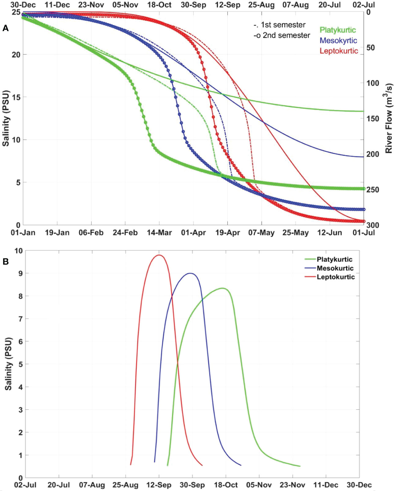
Figure 3 (A) A comparison of the mean over depth salinity averaged over a distance of 3 km from the river mouth between the three symmetric distributions. Bottom axis shows the dates of the 1st semester. The dotted lines denote salinity in the 1st semester. Top axis shows the dates of the 2nd semester moving from right to the left. Circled lines denote salinity in the 2nd semester increasing from right to the left. The river discharge of each symmetric distribution is added with continuous lines and with its scale on the right axis. The flow increases from 1st of January until 1st of July following the bottom axis and decreases from 2nd of July until 31 of December following the top axis. (B) A timeline of the salinity differences above 0.5 PSU between the 1st and 2nd semester for each symmetric distribution.

Figure 3A shows that initially, the order between the three symmetric distributions is as follows:

S_leptokurtic >S_mesokurtic > S_platykurtic because the relationship between the river discharge (Q) magnitude of the three symmetric distributions follows the opposite order Q_platykurtic > Q_mesokurtic > Q_leptokurtic. The order between the river discharges changes as the flow increases in the 1st semester and so does that of the salinity. S_leptokurtic falls below S_platykurtic at first and S_mesokurtic a few days later. The dates of the intersection between the salinity curves correspond to the dates of intersection between the flow curves in each case which means that the salinity becomes lower in one simulation when its flow becomes higher than the flow of another simulation.

The opposite procedure takes place at the 2nd semester and as long as the flow decreases. The salinity of the leptokurtic hydrograph becomes higher than the mesokurtic and then than the platykurtic salinity.

Figure 3A indicates that there is a hysteresis on the salinity’s response between increasing and decreasing flows. For example, the leptokurtic salinity falls below the platykurtic one in the 1st semester on the 5th of May. This means that the change occurs only 55 days before the peak flow day on the 1st of July. On the contrary, the leptokurtic salinity becomes higher than the platykurtic one in the 2nd semester on the 10th of September. This is 72 days far from the 1st of July (peak flow day) which shows a delay in comparison to the interchange in the 1st semester between the two simulations. Similar conclusions can be drawn when comparing between any couple of simulations.

In addition, it can be seen that there is a time frame in each simulation when the salinity in the 2nd semester is always lower compared to its corresponding date of equal flow in the 1st semester. This indicates that the salinity might not be equal at dates of equal flow depending on whether the flow is increasing or decreasing and whether the peak flow has occurred already or not. However, this effect is not present for very low flows (at the start of the simulation) or very high ones while getting closer to the peak flow day. In this case, the salinity is equal for equal flows independent of increasing or decreasing river discharge.

To get a clearer image of this salinity asymmetry between 1st and 2nd semester, the salinity differences of more than 0.5 PSU between the two semesters are plotted in Figure 3B for each day and each simulation separately. The maximum salinity difference increases with the peak flow magnitude, but the duration of salinity differences decreases with it. For example, differences in salinity between the two semesters can reach 10 PSU in the leptokurtic case but they are present only for approximately 1.5 months. On the contrary, the maximum salinity difference in the platykurtic case is 8 PSU but differences are present for 2.5 months instead.

3.1.2 Skewed hydrographs

The analysis for the two skewed hydrographs is presented in a different manner since the flow range remains the same in both cases. Figure 4 displays the salinity averaged over depth and over the radial cross section 3 km far from the mouth against the river discharge. The left skewed case shows almost equal salinity between the start and the end of the simulation. The long tail covers a period of 9 months with decreasing flows that allows the salinity to recover and return to its initial state. In contrast, the salinity for the right skewed hydrograph is about 1 PSU lower at the end of the simulation compared to its initial value. In this case, the simulation ends with the short tail that covers a period of only 3 months with a very sharp flow decrease that does not allow the salinity to recover.

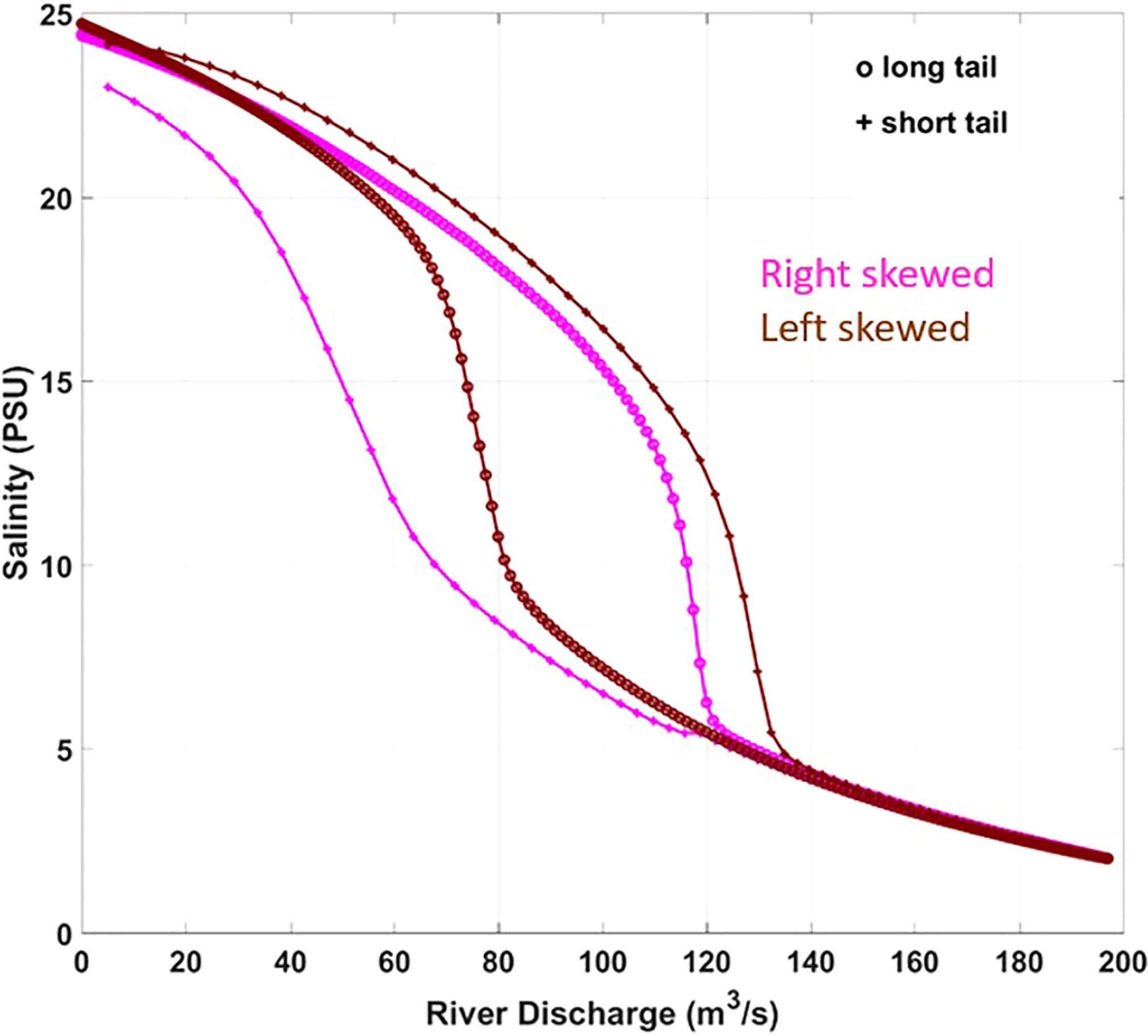
Figure 4 The mean over depth salinity averaged over a distance of 3 km far from the river mouth against the river discharge for the two skewed hydrographs. The circles correspond to the dates of the long tail and the crosses to those of the short tail.

There are indications of a hysteresis in salinity’s response to flow changes in Figure 4 as well. Both simulations exhibit a time frame with lower salinity during the decreasing flow periods compared to equal discharges at increasing flow periods. The salinity is lower in the short tail for the right skewed and in the long tail for the left skewed case.

Similar to what is observed in Figure 3A for the symmetric hydrographs, there is a flow range with equal salinity. This occurs during high flow periods. When the flow is between 120 m³/s and 200 m³/s the salinity is equal between the two skewed hydrograph simulations. This indicates that for very high flows, the salinity’s response is independent of skewness and of increasing or decreasing flows.

The flow range in the short and long tails is equal in both simulations and varies between very low discharges and the peak flow that is close to 200 m³/s. The short and long tail seem to cause the same level of salinity variation as this fluctuates between 0 PSU and 24 PSU implying that by increasing the flow rate a salinity standard could be achieved in much shorter time.

3.2 Stratification

Changes in the river discharge affect the stratification. Increases in the river discharge usually result in stronger stratification (Monismith et al., 2002; MacCready, 2004; Ralston et al., 2008; Lerczak et al., 2009; Wei et al., 2016) with high top to bottom density differences. Therefore, the influence of the flow distribution on the stratification is measured in this section by taking the difference of the top to bottom layer salinity. To visualize the results, the top to bottom salinity differences are averaged over radial cross-sections like it was done in section 3.1. The averaging is done over points in a distance of 3 km and 5 km from the river mouth (red and yellow semicircles in Figure 1F) to compare results between shallow locations in the delta front (i.e. area including delta channels) and deeper ones at the pro-delta (i.e. delta area beyond the channels ends) (Hori and Saito, 2007). The evolution in time of the stratification is presented for both symmetric and skewed flow distributions and for both radial sections in Figure 5.

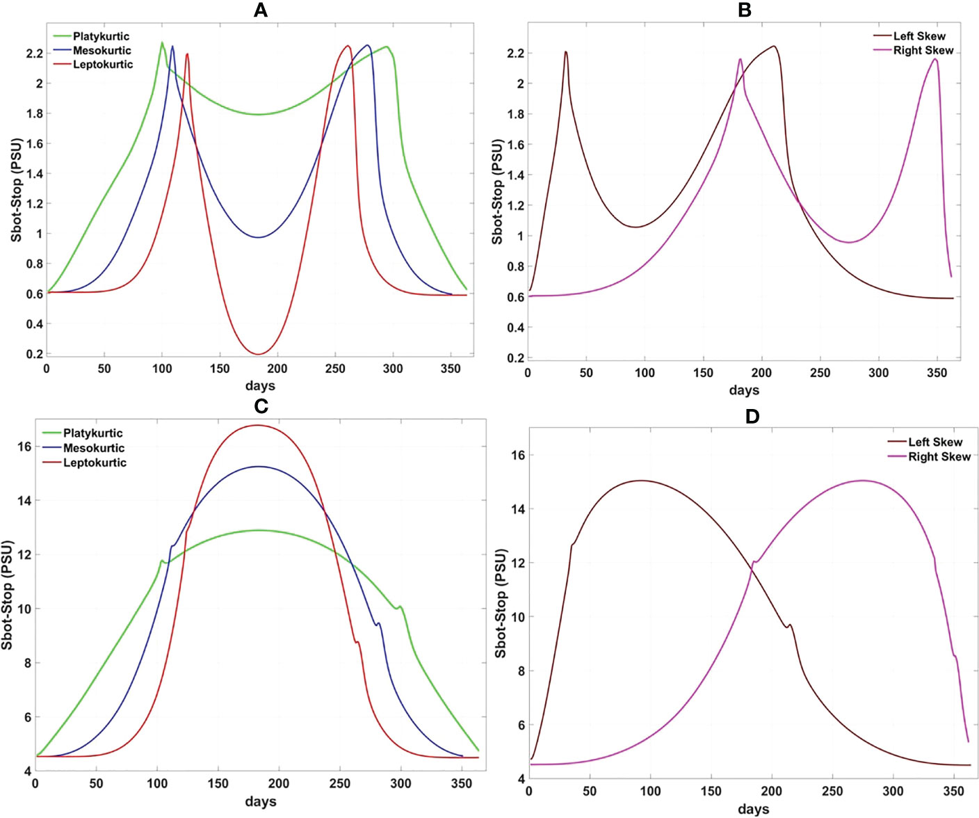
Figure 5 (A, B) The evolution in time of the top to bottom layer difference of the radially averaged salinity in a distance 3 km from the mouth in the symmetric and skewed flow distributions respectively. (C, D) The evolution in time of the top to bottom layer difference of the radially averaged salinity in a distance 5 km from the mouth in the symmetric and skewed flow distributions respectively.

The shape of the hydrograph does not seem to affect the range of stratification which remains similar between the five cases in each section (3km and 5km). This range is relatively small at the 3 km section (Figures 5A, B) which is the shallower one where mixing occurs under the influence of stronger bottom friction. The three symmetric hydrographs (Figure 5A) show a stratification level that increases initially following the hydrographs shape. For example, the leptokurtic curve demonstrates initially little change in stratification for as long as the low river discharges in the hydrograph’s tail (Figure 1C) do not differ much. At the same time, the platykurtic curve demonstrates a sharp increase of stratification in accordance with its hydrograph’s sharp flow increase (Figure 1A). As the river discharge increases continuously, it crosses a threshold above which it manages to mix the water column despite the absence of other contributors (e.g., tide-induced mixing). This is usually accompanied by a seaward shift of the salt intrusion length. The level of mixing depends on the level of the peak flow. The higher the peak the lower the stratification is. In that sense, the leptokurtic is the more efficient hydrograph against stratification while the decrease of stratification in the platykurtic is not substantial. The skewed hydrographs (Figure 5B) present similar results. Initially, the stratification increases following the flow increase but it drops when the river discharge is high enough to mix the waters. This occurs earlier in the left skewed case, 40 days after the start of the simulation and during the short tail. It occurs later in the right skewed simulation, 170 days after the start and during the long tail. In both cases, the stratification starts to increase again when the river discharge drops below a threshold value when it is not sufficient to mix the water anymore. After this point and till the end of the simulation, the top to bottom salinity differences follow the flow distribution.

In the deeper waters (5 km radial section, Figures 5C, D), the stratification follows the flow distribution and increases/decreases when the river discharge does increase/decrease too irrespective of the hydrograph shape. Its value reaches its maximum at the time of the peak flow. Accordingly, the higher the peak flow the higher the stratification can become, and this is why the leptokurtic shows the maximum top to bottom salinity difference (17 PSU) and the platykurtic the minimum one (13 PSU). In the same concept, the two skewed simulations (Figure 5D) show an equal maximum stratification occurring though at different time moments following the difference in the position of their peak on the hydrograph.

Changes in the spatial salinity distribution are reflected in Figures 5C, D as spikes, one before and another one after the peak flow. As the flow increases, the freshwater spreads radially in wider areas resulting in more symmetric spatial distributions. An example of a change in the spatial salinity distribution for the platykurtic hydrograph is given in the Supplementary Material (section 7.3). At the moment this change occurs, the rate of stratification increase/decrease in the 1st/2nd semester also changes. The time period between the spike and the peak flow is longer in the 2nd semester when the flow decreases as a result of the slower salinity’s response to decreasing than increasing flows.

3.3 Salt intrusion in the inlet

Sustained drought periods may result in salt intrusion inside the river mouth. This is often defined by the location of the 2 PSU bottom isohaline (Schubel, 1993; Monismith et al., 1996; Monismith et al., 2002; Herbold and Vendlinkski, 2012; Andrews et al., 2017). The time that the salinity at the bottom of the river mouth remains below 2 PSU is measured for each simulation with the intention to detect the flow distribution that keeps the river mouth fresh for the most time. Figure 2A shows the level of the bottom salinity at the river mouth (point A in Figure 1F) for the whole simulation period in each case. The five simulations start from a dry season state with very high salinity at the bottom of the mouth meaning that there is salt intrusion in the inlet. The intrusion is averted when the river flows become higher during the wet season. It is identified from Figure 2 that the river discharge at the time the salinity falls below 2 PSU is approximately 100 m³/s in each case. The rate at which the flow rises in each hydrograph until it reaches this threshold determines the moment that the inlet’s salt intrusion disappears first. The earliest this can happen is for the left skewed and the latest for the right skewed hydrograph. The time period that the inlet remains fresh is determined by the hydrographs’ tails and the peak flow position. Table 3 displays the total number of days and the days after the peak flow that the bottom salinity at the mouth is less than 2 PSU. The symmetric distributions indicate that the lighter the tails (platykurtic) the longer the inlet is fresh (210 days). The left skewed case, which also shows light tails but for shorter time, exhibits the second longer period (189 days). Being antisymmetric to the left, the right skewed hydrograph keeps the inlet fresh for a long period as well (179 days). However, the fact that its peak occurs much later in time seems to have an effect by cutting out 10 days making it equal to the mesokurtic hydrograph. The minimum duration of all (147 days) corresponds to the leptokurtic as it exhibits the heavier tails of all. The results are slightly different when the time is measured after the peak flow. In this case, the left skewed hydrograph exhibits the longer duration (126 days) with the platykurtic being second now (119 days). This indicates that it might be better to force a peak flow to occur early in the year in order to establish a freshwater system for longer periods. This is further supported by the indication that the right skewed hydrograph manages to keep the bottom salinity at the mouth below 2 PSU only for 80 days, even 2 days less than in the leptokurtic hydrograph.

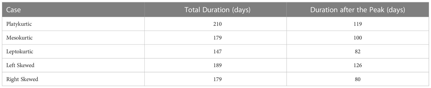
Table 3 The total duration and the time after the peak flow that the bottom salinity is less than 2 PSU at the river mouth.

3.4 Salinity longitudinal distribution

Possible effects of the hydrographs shape on the salinity longitudinal distribution are investigated in this section. In Figure 2B, the mean over depth and annual averages of salinity in the delta are averaged over radial cross sections every 300 m along a distance of 6 km from the river mouth (see cross-section AB in Figure 1F). This technique follows the concept of the salt intrusion curves, often used in other studies to measure cross-sectional salinity averages from the estuary mouth’s to its head (Savenije, 1993; Nguyen and Savenije, 2006; Nguyen et al., 2008; Zhang et al., 2011). The annual salinity average at the river mouth is above the 2 PSU threshold in every case. This is probably caused by the long periods of heavy tails (meaning very low flows) at all hydrographs except for the platykurtic one. Having the lightest tails of all, the platykutic case presents the lowest salinity value and closest to the 2 PSU threshold at the river mouth. The spatial salinity distribution in the delta increases gradually downstream. The rate of salinity increase between two successive sections is not constant because in contrast to their length, the depth of the radial cross-sections does not increase monotonously downstream. The shape of the five curves in Figure 2B is very similar and does not seem to be affected by the shape of the hydrograph. A border exists 4.2 km far from the river mouth where downstream of it the salinity is equal between the platykurtic, mesokurtic and the two skewed hydrographs. The green semi-circle in Figure 1F denotes the radial section of 4.2 km. This is located at the border between the delta front and the pro-delta. Upstream of this border, hydrographs with lighter tails (platykurtic) provide a salt intrusion curve of the lowest salinity. Hydrographs with almost equal peaks and flow ranges, such as the left skewed and the mesokurtic provide the exact same spatial salinity distribution in the delta. The salinity in the right skewed is slightly higher than them. A negative effect can be deduced then when moving the peak closer to the end instead of the start of the hydrograph as it causes an increase of salinity. Downstream of the green semicircle, in the absence of the complex channels’ bathymetry and in deeper waters (pro-delta), the salt intrusion curve is the same for all cases with the exception of the leptokurtic hydrograph that still shows the highest salinity. It appears then that the salinity in deep areas is less affected by changes in a hydrograph shape.

3.5 Freshwater residence time

Considering the water to be fresh as long as its salinity remains below 2 PSU, its residence time is calculated to determine how long the delta remains fresh in each simulation and to what extent. Figure 6 includes maps of the delta for each simulation displaying the total time in days that the depth averaged salinity remains below 2 PSU. The delta channels borders are delineated in the background (in black colour) to visualize the size of the area that becomes fresh in each case. The cyan color in these maps represents areas that never become fresh (freshwater RT is zero). In every case, the tendency is that the time salinity remains below 2 PSU decreases downstream in long distances from the river mouth. The peak flow seems to be the determinant factor for the extent that becomes fresh. This is almost the same for the mesokurtic (Figure 6B) and the two skewed cases (Figures 6D, E) because their maximum flows are very close (204 m³/s in the mesokurtic and 197 m³/s in the skewed hydrographs).

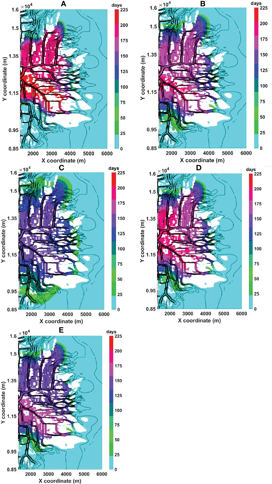
Figure 6 The time in days that salinity is less than 2 PSU in the delta for the (A)Platykurtic (B)Mesokurtic (C) Leptokurtic (D) Left and (E) Right skewed hydrograph cases. The black lines in the background delineate the delta channels. White coloured spaces denote dry areas. The river inlet has been taken out from the maps and the abscissa is set to start at the river mouth. Cyan coloured areas never become fresh.

In the symmetric distributions, the delta area that becomes fresh increases with increasing peak flow. Hence, every delta channel becomes fresh when the leptokurtic hydrograph is implemented - with the exception of the two most distant ones at the top left and bottom left corner of the map. On the contrary, a more limited delta area becomes fresh with the platykurtic hydrograph (Figure 6A) compared to the other hydrograph cases. Interestingly though, this case provides the longest freshwater conditions period. The delta is fresh in relatively small or medium distances from the mouth for almost 7 months. The freshwater duration period of a symmetric distribution decreases as the tails of the hydrograph become heavier. Therefore, the maximum time that salinity can be below 2 PSU with the leptokurtic hydrograph is only 5 months (Figure 6C). In the case of the skewed hydrographs the left one (Figure 6D) keeps the delta fresh for more time than the right (Figure 6E) highlighting the importance of its hydrograph slope that shows a rapid flow rise in the 1st semester and an early in time peak discharge. The hydrograph’s slope is identified as another crucial factor because the two cases exhibiting the faster rate of flow rise in the 1st semester (platykurtic and right skewed) provided the longer freshwater conditions in the delta.

In the map plots, differences in the duration within certain areas of the delta indicate bathymetry effects. There seems to be a difference of 25 days in the duration between the right and left sides of the inlet (looking seaward) (Figures 6A, B, D). The latter is deeper and thus the higher bottom salinity reduces the duration in comparison to the shallower areas right of the inlet. This difference is more pronounced in the right skewed case (Figure 6E) when the dry season is prolonged and the low freshwater flows do not manage to decrease the salinity in the deeper areas. On the other hand, this separation between deep and shallow areas is not present in the leptokurtic case (Figure 6C) because the peak flow is very high and can distribute symmetrically the fresh water throughout the delta.

3.6 Flushing times

Following the procedure discussed in section 2.6, the FT was measured twice after determining the averaging period first by setting the start at the day of the maximum flow and second at the last day of the simulation. Figure 7A displays the FT for both starting days. The five simulations show comparable results when the maximum flow day is considered the starting point. In this case, the averaging period is only one day because the river flow is so high that replaces immediately the salt with fresh water and so Q_F in equation 2 is also the Q_max. Consequently, the FTs are about 1 day and the differences between the five simulations are in the order of a few hours. The order of the FT magnitude between the five hydrographs follows the order of their peaks and the higher the flow the lower the FT is.

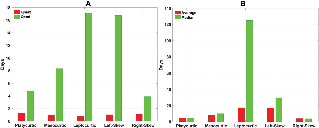
Figure 7 The flushing time for each simulation calculated using the Date Specific Method (DSM) to determine the river discharge averaging period. (A) Comparison of the flushing time measured with the average river discharge over a period with the starting date at the day of the maximum flow (Qmax, red bars) and the last day of the simulation (Qend, green bars). (B) Comparison of the flushing time measured with the average (red bars) and the median (green bars) river discharge over a period with a starting date at the last day of the simulation.

If the last day of the simulation is taken as the observation day to determine the averaging period, the differences in the FT between each hydrograph are more significant. The right skewed hydrograph exhibits the lowest FT (4 days) because it contains the highest flows at its end. The symmetric distributions show a progressive decrease of the FT as the hydrographs’ tails become lighter. As a result, the leptokurtic hydrograph requires the most time for water renewal (17 days) with the left skewed one demonstrating similar values since its heavy long tail occurs at the end of the simulation.

However, since most of the hydrographs contain very low river discharges at the end of their simulation, it is possible that the average discharge Q_end introduced in equation 2 might lead to an underestimation of the FT when the starting date is the last one. For this reason, the calculation of the FT is repeated for this specific case by introducing the median discharge over the averaging period instead of its mean value. Figure 7B provides a comparison between the FTs measured with the median and the average discharge. The outcome is very interesting because even though the relationship of the FTs between the various hydrographs remains the same, the values in some cases are quite different. In the leptokurtic case, the median FT is more than 120 days (4 months) while the average one was just 17 days. Clearly, the average discharge leads to an underestimation for a hydrograph with very heavy tails. Similarly, the left skewed hydrograph that also exhibits heavy tails at the end of the simulation gave a higher median FT (30 days) than its average one (17 days). In addition, the median FT uncovers a significant difference of the time required for water renewal between the leptokurtic and the left skewed hydrograph which was not detected when the average discharge was used. The left skewed hydrograph exchanges water 3 months faster than the leptokurtic according to the median FT calculation.

4 Discussion

4.1 Salinity response to river discharges

Results in section 3.1 indicate the existence of an asymmetry in the salinity response to flow changes. The salinity responds slower to decreasing than increasing flow independent of the hydrographs shape. This asymmetry has been identified in several estuarine studies as well (Blanton et al., 2001; Hetland and Geyer, 2004; Savenije, 2005; MacCready, 2007; Uddin and Haque, 2010; Chen, 2015). Savenije (2005) simply stated that the replacement of fresh with saltwater takes more time. Hetland and Geyer (2004) attributed the asymmetry in the estuarine response to the increase of the bottom drag when the flow decreases. The idealized delta presents a complex and asymmetric bathymetry so that it would be reasonable to assume an effect of the bottom drag to the salinity response. For example, Figure 6 shows higher freshwater RT in the shallower parts of the delta for some simulations. However, Figure 3A shows that this asymmetry does not concern periods with very high or very low flows. At these times, the salinity is equal for equal flows between the two semesters irrespective of whether the flow increases or decreases. The peak flow magnitude seems to have a strong influence. The higher the peak the shorter the asymmetry period is and the higher the salinity decreases too (Figure 3B). This may refer to the shorter adjustment times to large peaks in estuaries that Chen (2015) reported. In contrast to Hetland and Geyer (2004); Chen (2015) claims that the asymmetry is caused by two other factors: non-linearity of the salt flux and large variations in the river forcing. The results in section 3.1 present a direct dependence of the salinity response timescale to the flow. Monismith (2017) states that this is true only in systems close to steady state although the relationship is not linear. This is most probably true for the present case since the hydrographs of Figure 1 assume slow flow changes and this justifies the direct dependence of salinity response to river discharge observed in the results. In addition, Monismith (2017) examined if it is possible to take advantage of this asymmetry and achieve a specific salinity standard with flow variations of lower freshwater volumes compared to a constant flow for the same time frame. The outcome was that the flow needed to obtain a certain salinity value (e.g., 2 PSU) increases as the period of flow variation increases. Similarly, Figure 6C indicates that to sustain the 2 PSU salinity threshold in its most distant position, higher flow would be required to vary for a longer period. However, this would require an increased freshwater volume compared to that of the five hydrographs.

The response asymmetry of salinity to flow changes can be well detected in the skewed hydrographs too (Figure 4). The effect of high flow periods when the salinity does not vary between increasing or decreasing flows is also present. Most importantly though, the conclusion is that for a given flow range a standard salinity decrease could be achieved in much shorter time if the hydrographs tails become sharper or in other words if the flow rate is increased.

The latter outcome could be much useful in terms of water management as it seems that for a given flow range, the increase of its rate can decrease faster the salinity and improve remarkably the conditions in the delta. The faster rate of flow change (lighter tails) is also what probably makes the platykurtic hydrograph a preferable option compared to the leptokurtic one since it sustains freshwater conditions in the delta for longer periods. This would prolong the period that the various anthropogenic activities could take place safely in the delta even though the leptokurtic hydrograph could achieve larger salinity decrease but for a limited time.

4.2 Drivers of hydrographs shape change and its impact on salinity

Deltas can be found at all latitudes and climatic zones (Roberts et al., 2012). Although not absolute, a hydrograph’s shape could be indicative of certain climate zones. Climate change will affect hydrological regimes in the future which can reflect as changes in hydrographs shape. Riverine flow changes result from either natural climate variability (NCV) (Deser et al., 2012) or anthropogenic climate change (ACC) (Zhang and Delworth, 2018). NCV influences riverine floods magnitude and timing (Merz et al., 2014; Francois et al., 2019). Atmospheric processes such as intensified precipitation (Viglione et al., 2016) can increase riverine flood peak discharges (Hall et al., 2014; Zhang et al., 2015). Such increases may result in hydrographs like the leptokurtic in Figure 1C that presents a sharp peak. This type of hydrograph with large differences between maximum and minimum flows is often found in monsoonal climates (Hansford et al., 2020). The results analysis in section 3 indicates that peak flow increases could result in an offshore displacement of the salt intrusion length, freshening of a larger area in the delta, mixing of the water column with freshwater and fast renewal times during this period. However, this positive effect would be only temporary if it is not accompanied by an increase of the streamflow throughout the year and the delta’s salinity will shortly recover to its pre-peak flow state. A platykurtic hydrograph that has lower peak but smaller differences between maximum and minimum flows is more successful in retaining the delta fresh for longer periods. Increases of peak flows magnitude with thus similar effects may arise by ACC as well as for example urbanization and land use changes that decrease soil infiltration and weaken the natural buffering effect (Vogel et al., 2011; Prosdocimi et al., 2015; Francois et al., 2019).

Warmer temperatures have led to earlier spring discharges in rivers affected by snowmelt (IPCC, 2007; Matti et al., 2017; Bloschl et al., 2017). The left skewed hydrograph’s peak is of similar magnitude to the mesokurtic and the right skewed one but occurs earlier in time. An earlier occurrence of the same magnitude peak flow shows to have an advantage in terms of keeping the delta and its river mouth fresh for longer periods compared to the two other cases. Despite this, the annual and spatial averaged salinity remains the same between these three cases. Moreover, the earlier spring peak discharge shifts the river runoff away from the summer and the autumn which are the months with the highest water demand and so special consideration should be taken in these conditions (IPCC, 2007). On the other hand, polar warming has caused a delay of winter floods in the North Sea and some sectors in the Meditteranean Coast (Bloschl et al., 2017). In the hydrographs of Figure 1, when the peak flow is positioned late in time (right skewed) the freshwater residence time is much lower compared to other cases of equal peak flow. However, the winter’s water renewal time may become faster in this case because of the higher flows during this period.

Rises of temperature, increases of evaporation and warming of the oceans in recent years has intensified droughts that have also become more frequent (IPCC, 2007). In addition, reduction of runoff in many regions is assumed to be the result of a poleward expansion of the subtropical dry zone due to anthropogenic climate warming (Lu et al., 2007; Milly et al., 2008). Conversion of delta regions to arid zones due to sustained drought periods could modify their annual hydrographs into a mesokurtic shape which is the hydrograph type usually met in these zones (Hansford et al., 2020) as is the case for the Colorado and Nile deltas (Day et al., 2021). The effect on salinity would depend mainly on the peak flow change. If the peak flow increases then an offshore displacement of the salt intrusion zone should be expected, a decrease of stratification and freshwater residence times together with a delay in water renewal times. The reverse effects should be expected if the peak flow decreases.

4.3 Effects of flow distribution on stratification

The evolution of stratification in time with flow changes depends a lot on bathymetry. In deep waters, it follows the hydrographs shape consistent with what is reported in many estuarine studies (Monismith et al., 2002; MacCready, 2004; MacCready, 2007; Ralston et al., 2008; Lerczak et al., 2009; Wei et al., 2016). The level of stratification increases with the flow increase so that the leptokurtic hydrograph exhibits the maximum and the platykurtic the minimum top to bottom salinity differences. In shallow waters, the link between the stratification and the hydrograph shape breaks when the river discharge is sufficient to mix completely the water column. This is expected to happen in areas closer to the river mouth where the depth is shallower and the river discharge’s influence stronger. This difference of stratification between deep and shallow areas is not surprising and has been reported earlier. For example, Sridevi et al. (2015) observed something similar in the Godavari estuary where the top to bottom salinity differences varied along the estuary due to bathymetric differences. Stratification was higher in deeper stations and lower in the shallow ones. Several conclusions can be drawn considering this result.

If the interest regarding stratification is focused inside the delta and in areas closer to the river mouth, a flow distribution that follows the leptokurtic hydrograph shows several advantages. It presents longer periods with either mixed waters or very low vertical salinity differences compared to the other hydrographs. It should be noted though that during low flow periods, the salinity can be high despite low vertical differences. Special consideration should be taken then concerning the salinity thresholds of different activities taking place in the delta. The two skewed and the mesokurtic hydrographs demonstrate a very similar stratification range in accordance with their flow range. It could be deduced then that the level of stratification may be more sensitive to the peak flow magnitude than its position in the hydrograph.

The range of stratification is much higher in the deeper areas (Figures 5C, D) and that can be explained by the weakening of the bottom friction that leads to stronger stratification (Monismith et al., 1996; Shaha et al., 2012). Stratification may cause anoxic conditions at the bottom layers and low oxygen can have environmental consequences to the aquatic life (Chant, 2012). For example, riverine waters are responsible for recurrent summertime hypoxia at the bottom waters of the river dominated Mississippi Delta (Schiller et al., 2011). It is important to mention the absence of tides in this case because when present they contribute to vertical mixing reducing usually the stratification effects. For instance, active oxygen replenishment from the atmosphere is observed in the macrotidal Scheldt and Chikugo estuaries (Sun et al., 2020). It should be expected then that many of these conclusions could be relatively different in systems with high tide.

The same may apply if future sea level rise (SLR) scenarios are considered. SLR can strengthen the stratification as it is reported for example in the Pearl River Estuary (Hong et al., 2020). Shallower sections may become deep in certain SLR future scenarios, something that would increase stratification and thus require changes to water management to avert the subsequent implications. On the other hand, some recent studies suggest that the SLR effect on SI is often less significant than that of a decrease of upstream flows (Akter, 2019; Bellafiore et al., 2021). Flow seasonality must be considered as well when assessing the SLR effect as this is expected to be stronger during low discharge periods. For instance, in their modeling experiments, Bricheno et al. (2021) found that the SLR effect to SI in the Ganges-Brahmaputra-Ganges delta is enhanced during dry season but counteracted during wet season by an enhanced monsoon. For the same delta, Akter, 2019) identified a local impact to SI from SLR while decreases of the freshwater flow were found to affect the entire region.

4.4 Hydrograph shape effects on water renewal and freshwater residence times

The results of sections 3.5 and 3.6 indicate that each hydrograph type has certain advantages and disadvantages. Therefore, the decision on the selection of an optimum hydrograph regarding water quality should be per case and according to water management demands. The peak flow magnitude and the tails of each hydrograph are important parameters affecting freshwater RT and water renewal time. An incremental increase of the peak flow results in a seaward salt intrusion limit displacement due to the negative correlation between river discharge and salinity (Garvine et al., 1992; Wong, 1995; Liu et al., 2001; Monismith et al., 2002; Liu et al., 2007; Becker et al., 2010). This is reflected in the panels of Figure 6 as an increase of the freshwater area with the peak flow increase. The freshwater area and RT follow an opposite trend. An increase of the peak flow results in an increase of the freshwater area but decrease of the RT. This is a consequence of the heavier tails that the hydrographs with higher peak flows exhibit. For example, the leptokurtic hydrograph shows the lowest RT because of its sharp peak and the uneven flow distribution throughout the year. For the same reason, the leptokurtic dry season FT is also the maximum one since the freshwater cannot be fast enough replenished in such low flow conditions. Heavy tails cause also the leptokurtic hydrograph to present the maximum annual and space averaged salinity while the platykurtic shows the minimum.

Hydrographs of similar flow range and peak flows (e.g., skewed and mesokurtic) make fresh almost equal areas (Figure 6). However, the RT may vary between them because of bathymetry or the time of the peak flow in the hydrograph. For example, the left skewed hydrograph shows higher RT which indicates positive effect of an early peak river discharge. In contrast, when the peak flow is positioned at the end of the year (right skewness) the RT decreases significantly. In the last case, bathymetric effects are more pronounced because the difference in the RT between shallow and deeper areas is much higher than the two other cases.

Estimations of the water renewal time are important considering the increase in tracers transport times expected in the future for both seasons because of SLR (Hong and Shen, 2012; Chen et al., 2015; Ahn et al., 2018; Hong et al., 2020). Flushing times in estuaries and deltas are also expected to increase for the same cause. FT is known to vary a lot with seasonality (Ensign et al., 2004) and this results in different order of FTs between the five hydrographs during wet and dry season. FT gets shorter values during wet and higher during dry seasons.The critical parameters for the FT are the peak flow in the wet and the hydrographs tails in the dry season. However, the effect of the tails in the second case is much stronger than that of the peak discharges in the first case. The hydrographs shape does not significantly influence the FT during wet seasons. Although the FT decreases with the increase of the peak flow the difference is only within the range of hours. In contrast, the FT increases by days as the tails become heavier. The selection of the statistical river discharge value to be introduced in the freshwater fraction method equation is very important in the case of heavy tails such as those of the leptokurtic and left skewed hydrographs. The use of an average over a period of very low discharges such as those included in hydrographs with heavy tails can decrease the FT and provide an unrealistic estimation of the renewal time (Alber and Sheldon, 1999). The use of the median discharge is proposed instead. Table 4 summarizes the overall conclusions of the study by providing the basic advantages and disadvantages of each flow regime.

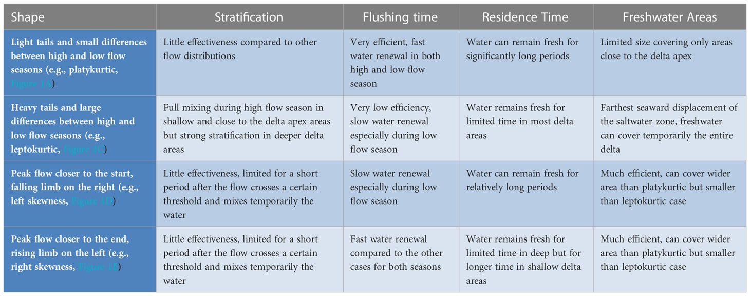
Table 4 A summary of the effects in stratification, flushing and residence times and freshwater areas caused by the main characteristics of the flow regimes under consideration.

5 Conclusions

In this study, the impact of different flow regimes on the salinity distribution in deltaic systems has been investigated. The work is motivated by the need to moderate saltwater intrusion consequences in deltas by better management of existing freshwater resources instead of resorting to expensive and harmful to the environment technical solutions. A 3D numerical model built in Delft3D for an idealized delta configuration was implemented for this purpose. Five test cases were considered, three of them with flow regimes of annual symmetric distribution but different flow range and two others with annual hydrographs of left and right skewness. To avoid complexity that could obscure direct conclusions, the simulations do not consider tides and Coriolis force was neglected. This may compromise the conclusions which might be then most applicable to river dominated deltas with little tidal influence and in medium latitudes.

The results analysis leads to interesting conclusions regarding the impact of various flow regimes on stratification, water renewal, freshwater area extent and residence times. In addition, the salinity response to flow changes has been assessed. It was found that the salinity responds slower to river discharge decreases than increases which is in accordance with what is stated in similar estuarine studies. The effect of flow regimes on stratification and mixing differs between shallow and deep areas in the delta. In deep waters and far from the delta apex, the top to bottom layer salinity difference follows the shape of the hydrograph and increases as the river discharge increases. In this case, leptokurtic and platykurtic hydrographs show the highest and lowest stratification level respectively following the difference in their peak flows. However, the reverse occurs in shallower and closer to the main trunk channel delta areas because the river discharge can mix the water column when crossing a certain flow threshold.

A hydrograph’s shape was found to be determinant factor for freshwater areas extent, renewal, and residence times. Platykurtic hydrographs present the maximum freshwater residence times because of their light tails (i.e., sharp flow increase) and small differences between maximum to minimum flow allowing an even water distribution throughout the year. The bathymetry is another crucial parameter as shallow areas remain fresh for longer periods. On the contrary, the extent of freshwater areas is determined by peak flows and therefore a leptokurtic hydrograph results in the farthest seaward displacement of the salt intrusion limit. Finally, the flow regime affects flushing times mainly during low flow periods. Water renewal becomes slower in the case of hydrographs with heavy tails (i.e., long periods with relatively low flows) rendering the leptokurtic hydrograph as the least efficient case. It was also discovered that the median instead of the mean over the averaging period river discharge results in more realistic and valid flushing times when hydrographs with very long low flow periods are considered.

The work in this paper indicates that it is possible to mitigate saltwater intrusion in deltas by applying water supply regulations. Each flow regime demonstrates different benefits for the various parameters under consideration (e.g., freshwater area and residence time) which should be accounted before any decisions for modifying existing hydrographs shape into another type. Nevertheless, the present study focuses on river flow forcing only and thus further research might be needed to determine the impact of other parameters such as for example tide-induced mixing and wind forcing.

Data availability statement

The original contributions presented in the study are publicly available. This data can be found here: https://zenodo.org/record/7373598#.Y9BAq3bP13gdoi:10.5281/zenodo.7373598.

Author contributions

CM: Conceptualization, Methodology, Software, Pre- and Post-processing, Visualization, Formal analysis, Writing, Original draft and reviewed versions preparation. LA: Supervision, reviewing and editing. LB: Supervision, reviewing and editing. NL: Supervision, reviewing and editing. All authors contributed to the article and approved the submitted version.

Funding

The work contained in this paper contains work conducted during a PhD study supported by the Natural Environment Research Council (NERC) EAO Doctoral Training Partnership whose support is gratefully acknowledged. Grant ref NE/L002469/1. Funding support from the School of Environmental Sciences, University of Liverpool are also gratefully acknowledged. For the purpose of Open Access, the author has applied a Creative Commons Attribution (CC BY) license to any Author Accepted Manuscript version arising.

Conflict of interest

The authors declare that the research was conducted in the absence of any commercial or financial relationships that could be construed as a potential conflict of interest.

Publisher’s note

All claims expressed in this article are solely those of the authors and do not necessarily represent those of their affiliated organizations, or those of the publisher, the editors and the reviewers. Any product that may be evaluated in this article, or claim that may be made by its manufacturer, is not guaranteed or endorsed by the publisher.

Supplementary material

The Supplementary Material for this article can be found online at: https://www.frontiersin.org/articles/10.3389/fmars.2023.1075683/full#supplementary-material

References

Adams W. (2000). World commission on dams, dams and development: A new framework for decision-making Vol. 1 (London: EarthScan), 1–28.
Ahmed M. F., Rahman M. M. (2000). Water supply and sanitation–rural and low-income urban communities. ITN–bangladesh, center for water supply and waste management, BUET, dhaka, bangladesh with contribution from IRC (The Netherlands: International Water and Sanitation Center, Delft).
Ahn D. T., Hoang L. P., Bui M. D., Rutschmann P.. (2018). Simulating future flows and salinity intrusion using combined one- and two-dimensional hydrodynamic modeling-the case of hau river, Vietnamese Mekong delta. Water 10 (7), 1–21. doi: 10.3390/w10070897
Akter R. (2019). The dominant climate change event for salinity intrusion in the GBM delta. Climate 7, 69. doi: 10.3390/cli7050069
Alber M., Sheldon J. E. (1999). Use of a date-specific method to examine variability in the flushing times of Georgia estuaries. Estuarine Coast. Shelf Sci. 49 (4), 469–482. doi: 10.1006/ecss.1999.0515
Allison L. E. (1964). Salinity in relation to irrigation. Adv. Agron. 16 (C), 139–180. doi: 10.1016/S0065-2113(08)60023-1
Andrews S. W., Gross E. S., Hutton P. H.. (2017). Modeling salt intrusion in the San Francisco estuary prior to anthropogenic influence’. Continental Shelf Research 146, 58–81. doi: 10.106/j.csr.2017.07.010
Balls P. W. (1994). ‘Nutrient inputs to estuaries from nine scottish east coast rivers; influence of estuarine processes on inputs to the north sea’. Estuarine Coast. Shelf Sci. 39, 329–352. doi: 10.1006/ecss.1994.1068
Banas N. S., Hickey B. M., MacCready P., Newton J. A.. (2004). Dynamics of willapa bay, Washington: A highly unsteady, partially mixed estuary. J. Phys. Oceanogr. 34 (11), 2413–2427. doi: 10.1175/JPO2637.1
Becker M. L., Luettich R. A. Jr, Mallin M. A.. (2010). Hydrodynamic behavior of the cape fear river and estuarine system: A synthesis and observational investigation of discharge-salinity intrusion relationships. Estuar. Coast. Shelf Sci. 88 (3), 407–418. doi: 10.1016/j.ecss.2010.04.022
Bellafiore D., Ferrarin C., Maicu F., Manfe G., Lorenzetti G., Umgiesser G., et al. (2021). Saltwater intrusion in a Mediterranean delta under a changing climate. J. Geophys. Res.: Oceans 126, e2020JC016437. doi: 10.1029/2020JC016437
Bhuiyan M. J. A. N., Dutta D. (2012). “Assessing impacts of sea level rise on river salinity in the gorai river network, Bangladesh,” in Estuarine, coastal and shelf science, vol. 96. (Elsevier Ltd), 219–227. doi: 10.1016/j.ecss.2011.11.005
Birkinshaw S. J., Guerreiro S. B., Nicholson A., Liang Q., Quinn P., Zhang L, et al. (2017). Climate change impacts on Yangtze river discharge at the three gorges dam. Hydrol. Earth Syst. Sci. 21 (4), 1911–1927. doi: 10.5194/hess-21-1911-2017
Blanton J., Alber M., Sheldon J.. (2001). Salinity response of the satilla river estuary to seasonal changes in freshwater discharge. Proceedings of the 2001 Georgia Water Resources Conference, held March 26-27, 2001, at the University of Georgia. Hatcher K. J. editor Athens, Georgia: Institute of Ecology, The University of Georgia.
Bloschl G., Hall J., Parajka J., Perdigao R. A., Merz B., Arheimer B., et al. (2017). Changing climate shifts timing of European floods. Science 357 (6351), 588–590. doi: 10.1126/science.aan2506
Bowen M. M. (2003). Salt transport and the time-dependent salt balance of a partially stratified estuary. J. Geophys. Res. 108 (C5), 1–15. doi: 10.1029/2001jc001231
Bricheno L. M., Wolf J., Islam S.. (2016). Tidal intrusion within a mega delta: An unstructured grid modeling approach. Estuarine Coast. Shelf Sci. 182, 12–26. doi: 10.1016/j.ecss.2016.09.014
Bricheno L. M., Wolf J., Sun Y.. (2021). Saline intrusion in the Ganges-Brahmaputra-Meghna megadelta. Estuarine Coast. Shelf Sci. 252, 107246. doi: 10.1016/j.ecss.2021.107246
Brockway R., Bowers D., Hoguane A., Dove V., Vassele V.. (2006). A note on salt intrusion in funnel-shaped estuaries: Application to the incomati estuary, Mozambique. Estuarine Coast. Shelf Sci. 66 (1–2), 1–5. doi: 10.1016/j.ecss.2005.07.014
Bryson M. (1974). Heavy tailed distributions: Properties and tests. Technometrics 16 (1), 61–68. doi: 10.1080/00401706.1974.10489150
Burpee A. P., Slingerland R. L., Edmonds D. A., Parsons D., Best J., Cederberg J.. (2015). Grain-size controls on the morphology and internal geometry of river-dominated deltas. J. Sediment. Res. 85 (6), 699–714. doi: 10.2110/jsr.2015.39
Caldwell R., Edmonds D. A. (2014). The effects of sediment properties on deltaic processes and morphologies: A numerical modeling study. J. Geophys. Res. 119 (5), 961–982. doi: 10.1002/2013JF002871.Received
Chant R. J. (2012). Interactions between estuaries and coasts: River plumes - their formation, transport, and dispersal, treatise on estuarine and coastal science (Elsevier Inc). doi: 10.1016/B978-0-12-374711-2.00209-6
Chen X. J. (2004). Modeling hydrodynamics and salt transport in the alafia river estuary, Florida during may 1999-December 2001. Estuarine Coast. Shelf Sci. 61 (3), 477–490. doi: 10.1016/j.ecss.2004.06.012
Chen W. B., Liu W. C., Hsu M. H. (2015). ‘Modeling assessment of a saltwater intrusion and a transport time scale response to sea-level rise in a tidal estuary’. Environ. Fluid Mech. 15, 491–514. doi: 10.1007/s10652-014-9367-y
Chen S. N. (2015). Asymmetric estuarine responses to changes in river forcing: A consequence of nonlinear salt flux. J. Phys. Oceanogr. 45 (11), 2836–2847. doi: 10.1175/JPO-D-15-0085.1
Chen X., Flannery M. S., Moore D. L.. (2000). Response times of salinity in relation to changes in freshwater inflows in the lower hillsborough river, Florida. Estuaries 23 (5), 735–742. doi: 10.2307/1352899
Chen X., Zong Y., Zhang E., Xu J., Li S.. (2001). Human impacts on the changjiang (Yangtze) river basin, China, with special reference to the impacts on the dry season water discharges into the sea. Geomorphology 41 (2), 111–123. doi: 10.1016/S0169-555X(01)00109-X
Choi K. W., Lee J. H. W. (2004). Numerical determination of flushing time for stratified water bodies. J. Mar. Syst. 50, 263–281. doi: 10.106/j.marsys.2004.04.005
Christian R. R., Boyer J. N., Stanley D. W. ’Multi-year distribution patterns of nutrients within the neuse river estuary. north carolina. Mar. Ecol. Prog. Ser. 71, 259–274. https://www.jstor.org/stable/24817298.
Clarke D., Williams S., Jahiruddin M., Parks K., Salehin M.. (2015). Projections of on-farm salinity in coastal Bangladesh. Environ. Sci.: Process. Impacts R. Soc. Chem. 17 (6), 1127–1136. doi: 10.1039/c4em00682h
Conner W. H., McLeod K.W., McCarron J. K. (1997). ‘Flooding and salinity effects on growth and survival of four common forested wetland species.’. Wetland Ecol. Manage. 5, 99–109.
Dai Z., Chu A., Stive M., Zhang X., Yan H.. (2011). Unusual salinity conditions in the Yangtze estuary in 2006: Impacts of an extreme drought or of the three gorges dam? Ambio 40 (5), 496–505. doi: 10.1007/s13280-011-0148-2
Das A., Justic D., Inoue M., Hoda A., Huang A., Park D. (2012). Impacts of Mississippi river diversions on salinity gradients in a deltaic Louisiana estuary: Ecological and management implications. Estuarine Coast. Shelf Sci. Elsevier Ltd 111, 17–26. doi: 10.1016/j.ecss.2012.06.005
Dasgupta S., Kamal F.A., Khan Z. H., Choudhury S., Nishat A.. (2015). River salinity and climate change: Evidence from coastal Bangladesh. World Sci. Ref. Asia World Econ., 205–242. doi: 10.1142/9789814578622_0031
Dawadi S., Ahmad S. (2013). Evaluating the impact of demand-side management on water resources under changing climatic conditions and increasing population. J. Environ. Manage. Elsevier Ltd 114, 261–275. doi: 10.1016/j.jenvman.2012.10.015
Day J. W., Barras J., Clairian E., Johnston J., Justic D., Kemp G. P., et al. (2005). Implications of global climatic change and energy cost and availability for the restoration of the Mississippi delta. Ecol. Eng. 24 (4 SPEC. ISS.), 253–265. doi: 10.1016/j.ecoleng.2004.11.015
Day J., Goodman R., Chen Z., Hunter R., Giosan L., Wang Y., et al. (2021). Deltas in Arid environments. Water 13 (12), 1677 (Switzerland: Water). doi: 10.3390/w13121677
Deltares (2014). Delft3D-flow: Simulation of multi-dimensional hydrodynamic flows and transport phenomena, including sediments. User Manual Hydro-Morphodynamics 3.15, 34158.
Deser C., Knutti R., Solomon S., Phillips A.S.. (2012). Communication of the role of natural variability in future north America climate. Natural Climate Change 2, 775–779. doi: 10.1038/NCLIMATE1562
Edmonds D. A., Slingerland R. L. (2010). “Significant effect of sediment cohesion on deltamorphology,” in Nature geoscience, vol. 3. (Nature Publishing Group), 105–109. doi: 10.1038/ngeo730
Eldardiry H., Hossain F. (2019). Understanding reservoir operating rules in the transboundary nile river basin using macroscale hydrologic modeling with satellite measurements. J. Hydrometeorol. 20 (11), 2253–2269. doi: 10.1175/JHM-D-19-0058.1
Ensign S. H., Halls J. N., Mallin M. A.. (2004). Application of digital bathymetry data in an analysis of flushing times of two large estuaries. Comput. Geosci. 30 (5), 501–511. doi: 10.1016/j.cageo.2004.03.015
Eslami S., Hoekstra P., Trung N. N., Kantoush S. A., Doan V. B., Do D. D, et al. (2019). Tidal amplification and salt intrusion in the Mekong delta driven by anthropogenic sediment starvation. Sci. Rep. 9 (1), 1–10. doi: 10.1038/s41598-019-55018-9
Eyre B., Twigg C. (1997). ‘Nutrient behaviour during post-flood recovery of the richmond river estuary northern NSW. Australia’. Estuarine Coast. Shelf Sci. 44 (3), 311–326. doi: 10.1006/ecss.1996.0124
Fischer H. B., List E. J., Imberger J., Koh R. C. Y., Brooks N. H. (1979). Mixing in inland and coastal waters (New York: Academic Press).
Francois B., Schlef K. E., Wi S., Borwn C. M.. (2019). Design considerations for riverine floods in a changing climate – a review. J. Hydrol. 547, 557–573. doi: 10.1016/j.jhydrol.2019.04.068
Frihy O. E. (2003). The nile delta-Alexandria coast: Vulnerability to sea-level rise, consequences and adaptation. Mitigation Adapt. Strat. Global Change 8 (2), 115–138. doi: 10.1023/A:1026015824714
Galloway W. E. (1975). “Process framework for describing the morphologic and stratigraphic evolution of deltaic depositional systems,” in Deltas: Model for exploration (Houston Geological Society), p.87–p.98.
Garvine R. W., McCarthy R. K., Wong K.. (1992). The axial salinity distribution in the delaware estuary and its weak response to river discharge. Estuarine Coast. Shelf Sci. 35 (2), 157–165. doi: 10.1016/S0272-7714(05)80110-6
Gleick P. H. (2003). Global freshwater resources: Soft-path solutions for the 21st century. Science 302 (5650), 1524–1528. doi: 10.1126/science.1089967
Glen S. (2016). “Heavy Tailed Distribution & Light Tailed Distribution: Definition & Examples,” in From StatisticsHowTo.com: Elementary Statistics for the rest of us! Available at: https://www.statisticshowto.com/heavy-tailed-distribution/.
Gong W., Shen J. (2011). “The response of salt intrusion to changes in river discharge and tidal mixing during the dry season in the modaomen estuary, China,” in Continental shelf research, vol. 31. (Elsevier), 769–788. doi: 10.1016/j.csr.2011.01.011
Gornitz V. (1991). Global coastal hazards from future sea level rise. Palaeogeogr. Palaeoclimatol. Palaeoecol. 89 (4), 379–398. doi: 10.1016/0031-0182(91)90173-O
Ha T. P., Dieperink C., Tri V. P. D, Otter H. S., Hoekstra P.. (2018). Governance conditions for adaptive freshwater management in the Vietnamese Mekong delta. J. Hydrol. 557, 116–127. doi: 10.1016/j.jhydrol.2017.12.024
Hagy J. D., Boynton W. R., Sanford L. P. (2000). ‘Estimation of net physical transport and hydraulic residence times for a coastal plain estuary using box models’. Estuaries 23 (3), 328–340. doi: 10.2307/1353325
Hall J., et al. (2014). Understanding flood regime changes in Europe: a state-of-the-art assessment. Hydrol. Earth Syst. Sci. 18, 2735–2772. doi: 10.5194/hess-18-2735-2014
Hansford M. R., Plink-Bjorklund P., Jones E. R.. (2020). “Global quantitative analyses of river discharge variability and hydrograph shape with respect to climate types,” in Earth-science reviews, vol. 200. (Elsevier), 102977. doi: 10.1016/j.earscirev.2019.102977
Herbold, Vendlinkski (2012). Modeling estuarine habitat in the bay delta, unifying one and three dimensional approaches to modeling X2 and the low salinity zone. Tech. Workshop Estuary Habitat.
Hetland R. D., Geyer W. R. (2004). An idealized study of the structure of long, partially mixed estuaries. J. Phys. Oceanogr. 34 (12), 2677–2691. doi: 10.1175/JPO2646.1
Hoitink A. J. F., Wang Z. B., Vermeulen B., Huismans Y., Kastner K.. (2017). Tidal controls on river delta morphology. Nat. geosci. 10, 637–645. doi: 10.1038/NGEO3000
Holm J., Sasser C. E. (2001). Differential salinity response between two Mississippi river subdeltas: Implications for changes in plant composition. Estuaries 24 (1), 78–89. doi: 10.2307/1352815
Hong B., Liu Z., Shen J., Wu H., Gong W., Xu H., et al. (2020). “Potential physical impacts of sea-level rise on the pearl river estuary, China,” in Journal of marine systems, vol. 201. (Elsevier), 103245. doi: 10.1016/j.jmarsys.2019.103245
Hong B., Shen J. (2012). “Responses of estuarine salinity and transport processes to potential future sea-level rise in the Chesapeake bay,” in Estuarine, coastal and shelf science, vol. 104–105. (Elsevier Ltd), 33–45. doi: 10.1016/j.ecss.2012.03.014
Hori K., Saito Y. (2007). “Classification, architecture and evolution of Large-river deltas,” in Large Rivers: Geomorphology and management. Ed. Gupta A. (John Wiley & Sons Ltd), 75–96.
Horner-Devine A. R., Hetland R. D., MacDonald D. G.. (2015). Mixing and transport in coastal river plumes. Annu. Rev. Fluid Mech. 47, 569–594. doi: 10.1146/annurev-fluid-010313-141408
Hu K., Ding P. (2009). The effect of deep waterway constructions on hydrodynamics and salinities in Yangtze estuary, China. J. Coast. Res. SPEC. ISSUE 56), 961–965.
Huang W. (2007). Hydrodynamic modeling of flushing time in a small estuary of north bay, florida, USA. Estuarine Coast. Shelf Sci. 74 (4), 722–731. doi: 10.1016/j.ecss.2007.05.016
Huang W., Spaulding M. (2002). ‘Modelling residence-time response to freshwater input in apalachicola bay, florida, USA’. Hydrological Processes 16 (15), 3051–3064. doi: 10.1002/hyp.1088
Hutton P. H., Rath S. J., Chen L., Ungs M. J., Roy S. B.. (2016). Nine decades of salinity observations in the San Francisco bay and delta: Modeling and trend evaluations. J. Water Resour. Plann. Manage. 142 (3), 1–11. doi: 10.1061/(ASCE)WR.1943-5452.0000617
IPCC (2007). “Climate change 2007: Impacts, adaptation and vulnerability,” in Contribution of working group II to the fourth assessment report of the intergovernmental panel on climate change, vol. ch1.3 . Eds. Parry M. L., Canziani O. F., Palutikof J. P., Linden P. J. v. d., Hanson C. E. (Cambridge, UK: Cambridge University Press), pp.85–pp111.
Jassby A. D., Kimmerer W. J., Monismith S. G., Armor C., Cloern J. E., Powell T. M.. (1995). Isohaline position as a habitat indicator for estuarine populations. Ecol. Appl. 5 (1), 272–289. doi: 10.2307/1942069
Kakoulaki G., MacDonald D., Horner-Devine A. R.. (2014). The role of wind in the near field and midfield of a river plume. Geophys.Res. Lett. 41, 5132–5138. doi: 10.1002/2014GL060606
Kaplan D., Munoz-Carpena R., Wan Y., Hedgepeth M., Zheng F., Roberts R., et al. (2010). Linking river, floodplain, and vadose zone hydrology to improve restoration of a coastal river affected by saltwater intrusion. J. Environ. Qual. 39 (5), 1570–1584. doi: 10.2134/jeq2009.0375
Kastner S. E. (2018). The influence of wind and waves on spreading and mixing in the Fraser river plume. J. Geophys. Res.: Oceans 123, 6818–6840. doi: 10.1029/2018JC013765
Kolker A., et al. (2018) The impacts of the Mississippi river and its delta on the oceanography, ecology and economy of the gulf of Mexico Large marine ecosystem. Available at: http://mississippiriverdelta.org/files/2018/08/Known-Impacts-of-the-Mississippi-River.pdf.
Lai X., Lai X., Huang Q., Zhang Y., Jiang J.. (2014). Impact of lake inflow and the Yangtze River flow alterations on water levels in Poyang Lake,China. Lake Reserv. Manage. 30 (4), 321–330. doi: 10.1080/10402381.2014.928390
Lamb M. P., Nittrouer J. A., Mohrig D., Shaw J.. (2012). Backwater and river plume controls on scour upstream of river mouths: implications for fluvio-deltaic morphodynamics. J. Geophys. Res. 117, F01002. doi: 10.1029/2011JF002079
Latrubesse E. M., Stevaux J., Sinha R.. (2005). Tropical rivers. Geomorphology 70 (3-4 SPEC. ISS.), 187–206. doi: 10.1016/j.geomorph.2005.02.005
Lebo M. E., Sharp J. H., Cifuentes L. A. (1994). ‘Contribution of river phosphate variations to apparent reactivity estimated from phosphate-salinity diagrams’. Estuarine Coast. Shelf Sci. 39, 583–594. doi: 10.1016/S0272-7714(06)80011-9
Leonardi N., Canestrelli A., Sun T., Fagherazzi S.. (2013). Effect of tides on mouth bar morphology and hydrodynamics. J. Geophys. Res.: Oceans 118 (9), 4169–4183. doi: 10.1002/jgrc.20302
Lerczak J. A., Geyer W. R., Ralston D. K.. (2009). The temporal response of the length of a partially stratified estuary to changes in river flow and tidal amplitude. J. Phys. Oceanogr. 39 (4), 915–933. doi: 10.1175/2008JPO3933.1
Lienou G., Mahe G., Dieulin C., Paturel J. E., Bamba F., Sighomnou D., et al. (2010). “The river Niger water availability: Facing future needs and climate change,” in Global change: facing risks and threats to water resources: Proceedings of the sixth world FRIEND conference, vol. 340. (Wallingford: AISH).
Liu W. C., Hsu M. H., Kuo A. Y., Kuo J. T.. (2001). The influence of river discharge on salinity intrusion in the tanshui estuary, Taiwan. J. Coast. Res. 17 (3), 544–552.
Liu W. C., Chen W. B., Cheng R. T., Hsu M. H., Kuo A. Y.. (2007). Modeling the influence of river discharge on salt intrusion and residual circulation in danshuei river estuary, Taiwan. Cont. Shelf Res. 27 (7), 900–921. doi: 10.1016/j.csr.2006.12.005
Liu B., Peng S., Liao Y., Wang H.. (2019). “The characteristics and causes of increasingly severe saltwater intrusion in pearl river estuary,” in Estuarine, coastal and shelf science, vol. 220. (Elsevier), 54–63. doi: 10.1016/j.ecss.2019.02.041
Liu Y., Chen H., Wang J., Yang S., Chen A.. (2020). Numerical simulation for the effects of waves and grain size on deltaic processes and morphologies. Open Geosci. 12 (1), 1286–1301. doi: 10.1515/geo-2020-0196
Lu J., Vecchi G. A., Reichler T.. (2007). Expansion of the Hadley cell under global warming. Geophys. Res. Lett. 34, L06805. doi: 10.1029/2006GL028443
MacCready P. (1999). Estuarine adjustment to changes in river flow and tidal mixing. J. Phys. Oceanogr. 29 (4), 708–726. doi: 10.1175/1520-0485(1999)029<0708:EATCIR>2.0.CO;2
MacCready P. (2004). Toward a unified theory of tidally-averaged estuarine salinity structure. Estuaries 27 (4), 561–570. doi: 10.1007/BF02907644
MacCready P. (2007). Estuarine adjustment. J. Phys. Oceanogr. 37 (8), 2133–2145. doi: 10.1175/JPO3082.1
Monismith S. G. (2017). An integral model of unsteady salinity intrusion in estuaries. J. Hydraulic Res. 55 (3), 392–408. doi: 10.1080/00221686.2016.1274682
Matsoukis C., Amoudry L. O., Bricheno L. M., Leonardi N.. (2022). Numerical investigation of river discharge and tidal variation impact on salinity intrusion in a generic river delta through idealized modelling. Estuaries Coasts 46, 57–83. doi: 10.1007/s12237-022-01109-2
Matti B., Dahlke H. E., Dieppois B., Lawler D. M., Lyon S. W.. (2017). Flood seasonality across Scandinavia – evidence of a shifting hydrograph? Hydrol. Process. 31, 4354–4370. doi: 10.1002/hyp.11365
McCabe R. M., MacCready P., Hickey B. M.. (2009). Ebb tide dynamics and spreading of a large river plume. J. Phys. Oceanogr. 39, 2839–2856.
Merz B., Aerts J., Arnbjerg-Nielsen K., Baldi M., Becker A., Bichet A., et al. (2014). Floods and climate: emerging perspectives for flood risk assessment and management. Natural Hazards Earth Syst. Sci. 14, 1921–1942. doi: 10.5194/nhess-14-1921-2014
Milly P. C. D., Betancourt J., Falkenmark M., Hirsch R. M., Kundzewicz Z. W., Lettenmaier D. P., Stouffer R., et al. (2008). Stationarity is dead: Whiter water management? Science 319, 573–574. doi: 10.1126/science.11519
Monismith S. G., Burau J. R., Stacey M. T. (1996). Stratification dynamics and gravitational circulation in northern San Francisco Bay. In: San Francisco Bay: The Ecosystem edited by Hollibaugh T. Washington, D. C.: Am. Assoc. for the Advance. of Sci., pp. 123–153.
Monismith S. G., Kimmerer W., Burau J. R., Stacey M. T.. (2002). Structure and flow-induced variability of the subtidal salinity field in northern San Francisco bay. J. Phys. Oceanogr. 32 (11), 3003–3019. doi: 10.1175/1520-0485(2002)032<3003:SAFIVO>2.0.CO;2
Montanari A. (2012). Hydrology of the po river: Looking for changing patterns in river discharge. Hydrol. Earth Syst. Sci. 16 (10), 3739–3747. doi: 10.5194/hess-16-3739-2012
Murray A. B. (2002). Seeking explanation affects numerical modeling strategies. Eos 83 (38), 418–419. doi: 10.1029/2002EO000304
Nguyen A. D., Savenije H. H. G., Pham D. N., Tang D. T.. (2008). “Using salt intrusion measurements to determine the freshwater discharge distribution over the branches of a multi-channel estuary: The Mekong delta case,” in Estuarine, coastal and shelf science, vol. 77. , 433–445. doi: 10.1016/j.ecss.2007.10.010
Nguyen A. D., Savenije H. H. G. (2006). Hydrology and earth system sciences salt intrusion in multi-channel estuaries: a case study in the Mekong delta, Vietnam. Hydrol. Earth Syst. Sci. 10, 743–754. doi: 10.5194/hess-10-743-2006
Nobi N., Das Gupta A. (1997). Simulation of regional flow and salinity intrusion in an integrated stream-aquifer system in coastal region: Southwest region of Bangladesh. Ground Water 35 (5), 786–796. doi: 10.1111/j.1745-6584.1997.tb00147.x
Phan T. D., Smart J. C. R., Sahin O., Capon S. J., Hadwen W. L.. (2018). Assessment of the vulnerability of a coastal freshwater system to climatic and non-climatic changes: A system dynamics approach. J. Cleaner Prod. 183, 940–955. doi: 10.1016/j.jclepro.2018.02.169
Pitlick J., Cress R. (2000). Longitudinal trends in channel characteristics of the Colorado river and implications for food-web dynamics (Grand Junction, Colorado: U.S. Fish and Wildlife Serv.)
Prosdocimi I., Kjeldsen T. R., Miller J. D.. (2015). ’Detection and attribution of urbanization effect on flood extremes using nonstationary flood-frequency models. Water Resour. Res. 51, 4244–4262. doi: 10.1002/2015WR017065
Qiu C., Zhu J. (2015). Assessing the influence of Sea level rise on salt transport processes and estuarine circulation in the changjiang river estuary. J. Coast. Res. 31 (3), 661–670. doi: 10.2112/JCOASTRES-D-13-00138.1
Rahman M. D. M, Mustafi M. A. A., Islam A. F.M.T, Mohammad N. (2014). The effect of rainfall, temperature and humidity on saline in the southern area of Bangladesh. Journal of Biology, Agriculture and Healthcare 4 (22), 58–61.
Rahman M. M., Penny G., Mondal M. S., Zaman M. H., Kryston A., Salehin M., et al. (2019). “Salinization in large river deltas: Drivers, impacts and socio-hydrological feedbacks,” in Water security, vol. 6. (Elsevier), 100024. doi: 10.1016/j.wasec.2019.100024
Ralston D. K., Geyer W. R., Lerczal J. A.. (2008). Subtidal salinity and velocity in the Hudson river estuary: Observations and modeling. J. Phys. Oceanogr. 38 (4), 753–770. doi: 10.1175/2007JPO3808.1
Roberts H. H, Weimer P., Slatt R. M.. (2012). River deltas, regional geology and tectonics (Elsevier B.V), 490–511. doi: 10.1016/B978-0-444-53042-4.00017-0
Sámano M. L., Barcena J. F., Garcia A., Gomez A. G., Alvarez C., Revilla J. A. (2012). Flushing time as a descriptor for heavily modified water bodies classification and management: Application to the huelva harbour. J. Environ. Manage. 107, 37–44. doi: 10.1016/j.jenvman.2012.04.022
Sarwar M. G. M. (2005). Impacts of Sea level rise on the coastal zone of Bangladesh ((Masters Programme in environmental science). (Sweden: Lund University).
Savenije H. H. G. (1993). Predictive model for salt intrusion in estuaries. J. Hydrol. 148 (1–4), 203–218. doi: 10.1016/0022-1694(93)90260-G
Savenije H. H. G. (2005). Salinity and tides in alluvial estuaries (Delft University of Technology), 8.
Schiller R. V., Kourafalou V. H., Hogan P., Walker N. D. (2011). The dynamics of the mississippi river plume: Impact of topography, wind and offshore forcing on the fate of plume waters. J. Geophysical Research: Oceans 116 (6), 1–22. doi: 10.1029/2010JC006883
Schubel J. R. (1992). Managing freshwater discharge to the San Francisco Bay/ Sacramento San Joaquin delta estuary the scientific basis for an estuarine standard. In Conclusions and recommendations of members of the scientific,policy, and management communities of the bay/delta estuary. United States Environmental Protection Agency.
Shaha D. C., Cho Y. K., Kim T. W., Valle-Levinson A.. (2012). Spatio-temporal variation of flushing time in the sumjin river estuary. Terrestrial Atmos. Ocean. Sci. 23 (1), 119–130. doi: 10.3319/TAO.2011.08.22.01(Hy
Shaw J. B., Mohrig D., Whitman S. K.. (2013). The morphology and evolution of channels on the wax lake delta, Louisiana, USA. J. Geophys. Res.: Earth Surf. 118 (3), 1562–1584. doi: 10.1002/jgrf.20123
Sheldon J. E., Alber M. (2006). The calculation of estuarine turnover times using freshwater fraction and tidal prism models: A critical evaluation. Estuaries Coasts 29 (1), 133–146. doi: 10.1007/BF02784705
Sheldon J. E., Alber M. (2002). A comparison of residence time calculations using simple compartment models of the altamaha river estuary, georgia. Estuaries 25 (68), 1304–1317.
Sherin V. R. (2020). “Recent salinity intrusion in the Bengal delta: Observations and possible causes,” in Continental shelf research, vol. 202. (Elsevier Ltd), 104142. doi: 10.1016/j.csr.2020.104142
Sitharam T. G., Yang S. Q., Falconer R., Sivakumar R., Jones B., Kolathayar S., et al. (2020). Sustainable water resource development using coastal reservoirs. Matthew Deans Butterworth-Heinemann.
Smedema L. K., Shiati K. (2002). Irrigation and salinity: A perspective review of the salinity hazards of irrigation development in the arid zone. Irrig. Drain. Syst. 16 (2), 161–174. doi: 10.1023/A:1016008417327
Spicer P., Cole K. L., Huguenard K., MacDonald D. G., Whitney M.. (2022). Wind effects on near- and midfield mixing in tidally pulsed river plumes. J. Geophys. Res.: Oceans 127, e2022JC018462. doi: 10.1029/2022JC018462
Sridevi B., Sarma V. V. S. S., Murty T. V. R., Sadhuram Y., Reddym N. P. C., Vijayakumar K.. (2015). Variability in stratification and flushing times of the gautami–godavari estuary, India. J. Earth Syst. Sci. 124 (5), 993–1003. doi: 10.1007/s12040-015-0594-5
Sun J., Liu L., Lin J., Lin B., Zhao H. (2020). Vertical water renewal in a large estuary and implications for water quality. Sci. Total Environ. 710, 1–12. doi: 10.1016/j.scitotenv.2019.135593
Tabarestani M. K., Fouladfar H. (2021). Numerical modeling of salinity changes in the desalination stage of a coastal reservoir. J. Hydraul 16 (3), 69–83. doi: 10.30482/JHYD.2021.281280.152110.30482/JHYD.2021.281280.1521
Trieu T. T. N., Phong N. T. (2015). The impact of climate change on salinity intrusion and pangasius (Pangasianodon hypophthalmus) farming in the Mekong delta, Vietnam. Aquacult. Int. 23 (2), 523–534. doi: 10.1007/s10499-014-9833-z
Uddin M., Haque A. (2010). Salinity response in southwest coastal region of Bangladesh due to hydraulic and hydrologic parameters. Int. J. Sustain. Agric. Technol. 6 (3), 1–7.
Uncles R. J., Stephens J. A. (1996). Salt intrusion in the Tweed estuary. Estuarine Coast. Shelf Sci. 43 (3), 271–293. doi: 10.1006/ecss.1996.0070
Valle-Levinson A., Wilson R. E. (1994). Effects of sill processes and tidal forcing on exchange in eastern long island sound. J. Geophys. Res. 99 (C6), 12667–12681. doi: 10.1029/94jc00721
Viglione A., Merz B., Dung N. V. D., Parajka J., Nester T., Bloschl G.. (2016). Attribution of regional flood changes based on scaling fingerprints. Water Resour. Res. 52 (7), 5322–5340. doi: 10.1002/2016WR019036
Visser J. M., Day J. W., Battaglia L. L, Shaffer G. P., Hester M. W.. (2012). “Mississippi River Delta Wetlands,” in book:Wetland Habitats of North America Ecology and Conservation Concerns Edition 1st, ch.5. Batzer D., Baldwin A. Editors. University of California Press, 63–74. doi: 10.1525/9780520951419-007
Vogel R. M., Yaindl C., Walter M.. (2011). Nonstationarity: flood magnification and recurrence reduction factors in the united states. J. Am. Water Resour. Assoc. 47 (3), 464–474. doi: 10.1111/j.1752-1688.2011.00541.x
Wang H., Krauss K. W., Noe G. B., Stagg C. L., Swarzenski C. M., Duberstein A. A., et al. (2020). Modeling soil porewater salinity response to drought in tidal freshwater forested wetlands. J. Geophys. Res.: Biogeosci. 125 (2). doi: 10.1029/2018JG004996
Wei X., Schramkowski P., Schuttelaars H. M.. (2016). Salt dynamics in well-mixed estuaries: Importance of advection by tides. J. Phys. Oceanogr. 46 (5), 1457–1475. doi: 10.1175/JPO-D-15-0045.1
Wei X., Kumar M., Schuttelaars H. M.. (2017). Three-dimensional salt dynamics in well-mixed estuaries: Influence of estuarine convergence, Coriolis and bathymetry. J. Phys. Oceanogr. 47, 1843–1871. doi: 10.1175/JPO-D-16-0247.1
Weisberg M. (2007). Three kinds of idealization. J. Philosophy 104 (12), 639–659. doi: 10.5840/jphil20071041240
Williams B. L. (1986). Flushing time calculations for the upper waitemata harbour, new zealand. New Z. J. Mar. Freshw. Res. 20 (3), 455–465. doi: 10.1080/00288330.1986.9516165
White E. D., Meselhe E., Reed D., Renfro A., Snider N. P., Wang Y.. (2019). Mitigating the effects of sea-level rise on estuaries of the Mississippi delta plain using river diversions. Water 11 (10), 2028. doi: 10.3390/w11102028
Wong K. C. (1995). On the relationship between long-term salinity variations and river discharge in the middle reach of the delaware estuary. J. Geophys. Res.: Oceans 100 (C10), 20,705–20,713. doi: 10.1029/95JC01406
Yang Y. C. E., Ray P. A., Brown C. M., Khalil A. F., Yu W. H.. (2015). Estimation of flood damage functions for river basin planning: a case study in Bangladesh. Natural Hazards 75 (3), 2773–2791. doi: 10.1007/s11069-014-1459-y
Yuan Y., Avener M. E., Horner-Devine A. R.. (2011). A two-color optical method for determining layer thickness in two interacting buoyant plumes. Exp. .Fluids 50, 235–1245. doi: 10.1007/s00348-010-0969-y
Yuan J. Z., Wu C. (2020). “Insights into the design and development of shanghai coastal reservoirs,” in Sustainable water resource development using coastal reservoirs (Elsevier Inc), 97–110. doi: 10.1016/b978-0-12-818002-0.00006-x
Yue S., Ouarda T. B. M., Bobee B., Legendre P., Bruneau P.. (2002). Approach for describing statistical properties of flood hydrograph. J. Hydrol. Eng. 7 (2), 147–153. doi: 10.1061/(ASCE)1084-0699(2002)7:2(147
Zevenbergen C., et al. (2018). Adaptive delta management: a comparison between the Netherlands and Bangladesh delta program. Int. J. River Basin Manage. Taylor Francis 16 (3), 299–305. doi: 10.1080/15715124.2018.1433185
Zhang H., Delworth T. L. (2018). Robustness of anthropogenically forced decadal precipitation changes projected for the 21st century. Nat. Commun. doi: 10.1038/s41467-018-03611-3
Zhang E., Savenije H. H. G., Wu H., Kong Y., Zhu J.. (2011). “Analytical solution for salt intrusion in the Yangtze estuary, China,” in Estuarine, coastal and shelf science, vol. 91. (Elsevier Ltd), 492–501. doi: 10.1016/j.ecss.2010.11.008
Zhang Q., Gu X., Singh V. P., Xiao M., Chen X.. (2015). ’Evaluation of flood frequency under non-stationarity resulting from climate indices and reservoir indices in the East river basin, China. J. Hydrol. 527, 565–575. doi: 10.1016/j.jhydrol.2015.05.029
Zhou X., et al. (2017). “Prospective scenarios of the saltwater intrusion in an estuary under climate change context using Bayesian neural networks,” in Stochastic environmental research and risk assessment, vol. 31. (Berlin Heidelberg: Springer), 981–991. doi: 10.1007/s00477-017-1399-7
Keywords: river deltas, salt intrusion, idealized modeling, flow regimes, water management
Citation: Matsoukis C, Amoudry LO, Bricheno L and Leonardi N (2023) Investigating how river flow regimes impact on river delta salinization through idealized modeling. Front. Mar. Sci. 10:1075683. doi: 10.3389/fmars.2023.1075683
Received: 20 October 2022; Accepted: 10 January 2023;
Published: 02 February 2023.
Edited by:
Yi Pan, Hohai University, ChinaReviewed by:
Beatrice M.S. Giambastiani, University of Bologna, ItalyJosé Pinho, University of Minho, Portugal
Copyright © 2023 Matsoukis, Amoudry, Bricheno and Leonardi. This is an open-access article distributed under the terms of the Creative Commons Attribution License (CC BY). The use, distribution or reproduction in other forums is permitted, provided the original author(s) and the copyright owner(s) are credited and that the original publication in this journal is cited, in accordance with accepted academic practice. No use, distribution or reproduction is permitted which does not comply with these terms.
*Correspondence: Constantinos Matsoukis, cm262@stir.ac.uk