Chlorophyll and POC in polar regions derived from spaceborne lidar

Highlights

- New FFNN algorithm was proposed to retrieve bbp, Chl, and POC from spaceborne lidar

- CALIPSO measurements in the polar regions fill the gap of passive measurements

- Comparison with in situ data indicates that FFNN-based lidar products perform well

- Combined description of annual cycles of bbp, Chl, and POC in polar regions

- Analysis of key factors governing phytoplankton growth in polar regions

1 Introduction

Marine phytoplankton plays a key role in the marine food web and biogeochemical cycles (Xu et al., 2020) and its photosynthetic production of organic carbon is vital for regulating atmospheric carbon dioxide (Parekh et al., 2006). Changes in phytoplankton primary production have a critical impact on higher trophic levels like zooplankton and ichthyoplankton (Capuzzo et al., 2018). As a commonly used proxy of phytoplankton abundance (Gordon et al., 1980; Li et al., 2022), the chlorophyll concentration (Chl) is traditionally estimated by passive ocean color remote sensing measurements for long-term studies (Alvera-Azcárate et al., 2021). In fact, ocean color remote sensing has reshaped our understanding of upper-ocean biogeochemistry for the global oceans as well as in regional basins (Dickey et al., 2006; McClain, 2009; Blondeau-Patissier et al., 2014; Brewin et al., 2017; Jackson et al., 2017). However, passive remote sensing can only work during the daytime because of the need for sunlight (Jamet et al., 2019), which leaves vast high-latitude ocean areas unobserved during lengthy polar nights. As a result, only a limited amount of data is available for polar regions.

Recently, an active remote sensing technique, light detection and ranging (lidar) has drawn great attention because of its independence from sunlight, which could address the limitations of passive remote sensing. In practice, spaceborne lidar CALIOP has shown remarkable potential in research of ocean carbon stocks (Behrenfeld et al., 2013) and phytoplankton biomass (Behrenfeld et al., 2017). However, previous studies heavily relied on the CALIOP particulate backscatter coefficient (bbp) to derive total particulate organic carbon (POC) and phytoplankton biomass. Besides, CALIOP bbp inversion method needs to assume the conversion factor used to derive bbp from the backscatter coefficient at 180° (b_π ) (Behrenfeld et al., 2019; Bisson et al., 2021). However, variabilities and inconsistencies of the conversion coefficient affect uncertainties to the retrieval of CALIOP bbp substantially (Berthon et al., 2007; Sullivan and Twardowski, 2009; Zhang et al., 2012; Chami et al., 2014; Hu et al., 2020).

This study intends to propose an innovative feed-forward neural network (FFNN) method to retrieve bbp, Chl, and POC from CALIOP measurements and study the interannual variability of phytoplankton based on the CALIOP-derived estimates of ocean variables. The remainder of the manuscript is organized as follows: data and methods are described in Section 2; after validation of the accuracy of the proposed method, the interannual variability is studied in Section 3; a discussion about the key factors governing phytoplankton growth in polar regions is presented in Section 4; conclusions and perspectives are provided in Section 5.

2 Materials and methods

2.1 Data

The data including CALIOP Level-1B V4.1 data products, Level-2 Merged Layer V4.20 products, and MODIS Level-3 9 km monthly averaged data are mainly used here. Launched in April 2006, CALIPSO flew in the “A-Train” constellation and followed Aqua within 2 minutes (Kim et al., 2013), which provided for near-simultaneous observations between them. As the main payload onboard CALIPSO, CALIOP is a nadir-pointing two-wavelength polarization-sensitive elastic backscatter lidar. CALIOP provides attenuated backscatter at 532 nm perpendicular component, 532 nm parallel component, and 1064 nm. The receiver footprint diameter is 90 m and the horizontal resolution is 333 m (Winker et al., 2009). The vertical resolution in water is 22.5 m (Lu et al., 2014). CALIOP Level-1B V4.1 product, which has significantly improved calibration accuracy compared with previous versions (Getzewich et al., 2018), is used for the ocean optic property inversion. Level-2 Merged Layer V4.20 product provides integrated attenuated backscatter (IAB) and aerosol optical depth (AOD) parameters.

MODIS is a key instrument aboard the Terra and Aqua satellite. As Aqua flies in the “A-Train” constellation as well, only MODIS products onboard Aqua are used for the simultaneity between different observations. The algorithms developed for the inversion bbp include Garver-Siegel-Maritorena algorithm (GSM) (Maritorena et al., 2002), Quasi Analytical Algorithm (QAA) (Lee et al., 2002), and Generalized Inherent Optical Property algorithm (GIOP) (Werdell et al., 2013). Since GIOP outperformed other inversion methods (Bisson et al., 2019), MODIS GIOP b_bp443 L3 9 km product is used here. MODIS POC is produced using blue-to-green band ratios (Stramski et al., 2008). MODIS Chl is derived based on the standard Ocean Color Chlorophyll (OC2) (O'Reilly et al., 1998) band ratio algorithm merged with the color index (CI) (Hu et al., 2012). In situ Chl were obtained from biogeochemical Argo data (Claustre et al., 2019) available from the Argo Data Assembly Center (ftp://ftp.ifremer.fr/ifremer/argo/dac/, last access: 20 May 2022) and used to validate the lidar-derived results. The spatial distribution of in situ data is shown in Supplementary Figure 1A, where blue dots represent all in situ data and red asterisks represent the matched data. Histograms of all data and matched data are shown in Supplementary Figures 1B, C. The mean values of all data and matched data are 0.50 mg/m³ and 0.81 mg/³, respectively. Sea ice extend is obtained from the Copernicus Climate Change Service (https://climate.copernicus.eu/sea-ice, last access: 5 June 2022) which is derived based on EAR5 (Hersbach et al., 2020; Bell et al., 2021). Estimates of photosynthetically available radiation (PAR) are from NASA Ocean Color website (https://oceancolor.gsfc.nasa.gov/, last access: 7 June 2022) that are derived from MODIS (Frouin et al., 2012). Monthly global reprocessed products of physical variables from ARMOR3D L4 distributed through the Copernicus Marine Environment Monitoring Service (https://resources.marine.copernicus.eu/product-detail/MULTIOBS_GLO_PHY_TSUV_3D_MYNRT_015_012, last access: 7 June 2022) are used for sea surface temperature (SST) and mixed layer depth (MLD).

2.2 Methods

2.2.1 CALIOP data preprocessing

For CALIOP data, the backscatter signal separated by the polarization beam splitter (PBS) at 532 nm is detected by photomultiplier tubes (PMTs). Due to the transient response of the detector, the subsequently measured signal intensity following the signal peak is greater than the true backscatter signal. The measured signal should be corrected by using deconvolution as follows (Lu et al., 2014):

where β^′(z) is the corrected backscattered signal, β(z) is the measured signal and [F] is the matrix form of the transient function.

Due to the polarization crosstalk caused by the nonideal characteristics of PBS, a portion of the parallel polarization component is transformed into the perpendicular component. The effects of crosstalk can be removed as follows:

where β_∥,c and β_⊥,c are corrected parallel and perpendicular signals, respectively. β_∥,m and β_⊥,m are measured parallel and perpendicular signals, respectively.

Then, the subsurface column-integrated backscatter of the perpendicular components, βw₊ can be calculated as follows (Behrenfeld et al., 2013):

where, βs is the lidar surface backscatter that can be evaluated using co-located surface wind speed (Hu et al., 2008). δ_T is the total column-integrated depolarization ratio that can be calculated as follows (Dionisi et al., 2020):

where p is the range bin of the peak surface return.

Generally, CALIOP bbp estimates were based on β;w₊, which has ${\text{b}}_{\text{bp}}^{\text{CALIOP}}\approx \frac{{\beta }_{w+}}{0.32* {0.98}^2 }$ (Bisson et al., 2021). However, the conversion coefficient of 0.32 has its uncertainty and inconsistency. This value was reported as 1.43 in some studies (Sullivan and Twardowski, 2009; Zhang et al., 2014), or 1.06 in some other studies (Lee et al., 2013; Churnside et al., 2014; Churnside and Marchbanks, 2015). While others reported a value of 0.5 (Boss and Pegau, 2001; Chami et al., 2006; Whitmire et al., 2010). The variability of the conversion coefficient may introduce uncertainties to the retrieval of CALIOP bbp. Compared with previous studies, the nonlinear deep neural network algorithm does not require predetermined knowledge, which could be an effective alternative method.

2.2.2 Network configuration and evaluation protocol

In previous studies, CALIOP bbp was calculated based on β;w₊ (Lu et al., 2014; Bisson et al., 2021). Then, POC and phytoplankton biomass were estimated based on CALIOP bbp (Behrenfeld et al., 2013; Behrenfeld et al., 2017). The FFNN algorithm is used here to derive bbp, POC, and Chl from β;w₊ directly. Previous studies showed that δ_T parameters can provide valuable information about bbp and Chl (Dionisi et al., 2020). Overall, β;w₊, δ_T and latitude are used as input variables (or predictors). The FFNN algorithm could adjust the relationship between the output and CALIOP variables in terms of latitude (Murphy and Hu, 2021). As shown in Figure 1, a multilayer perceptron using a backpropagation network (MLP BPN) is used for the FFNN model. The model comprises an input layer, 10 hidden layers, and an output layer. The hidden layers have 100 nodes each. The configuration of the model is based on a series of tests and their statistical results. A sigmoid function was chosen as an activation function for neurons in hidden layers (Sharma et al., 2020), and a linear function was used for the output layer to generate the final results. The model was trained by using the optimization algorithm of root mean square prop (RMSprop) which divides the gradient by a running average of its recent magnitude (Hinton et al., 2012). In this study, CALIPSO lidar backscatter measurements at daytime in 2008 and collocated b_bp, POC, and Chl products from Aqua/MODIS are used for the training model. CALIOP variables are averaged 9 km along-track to match the MODIS data. There are 1,144,878 matched points and the dataset was randomly divided into 70% for FFNN training, 15% for model validation, and 15% for its evaluation. The evaluation data did not participate in the training. As shown in Supplementary Figure 2, the matched data cover almost all of the global oceans. Then, the FFNN algorithm is applied to b_bp, POC, and Chl inversion between 2008 and 2021.

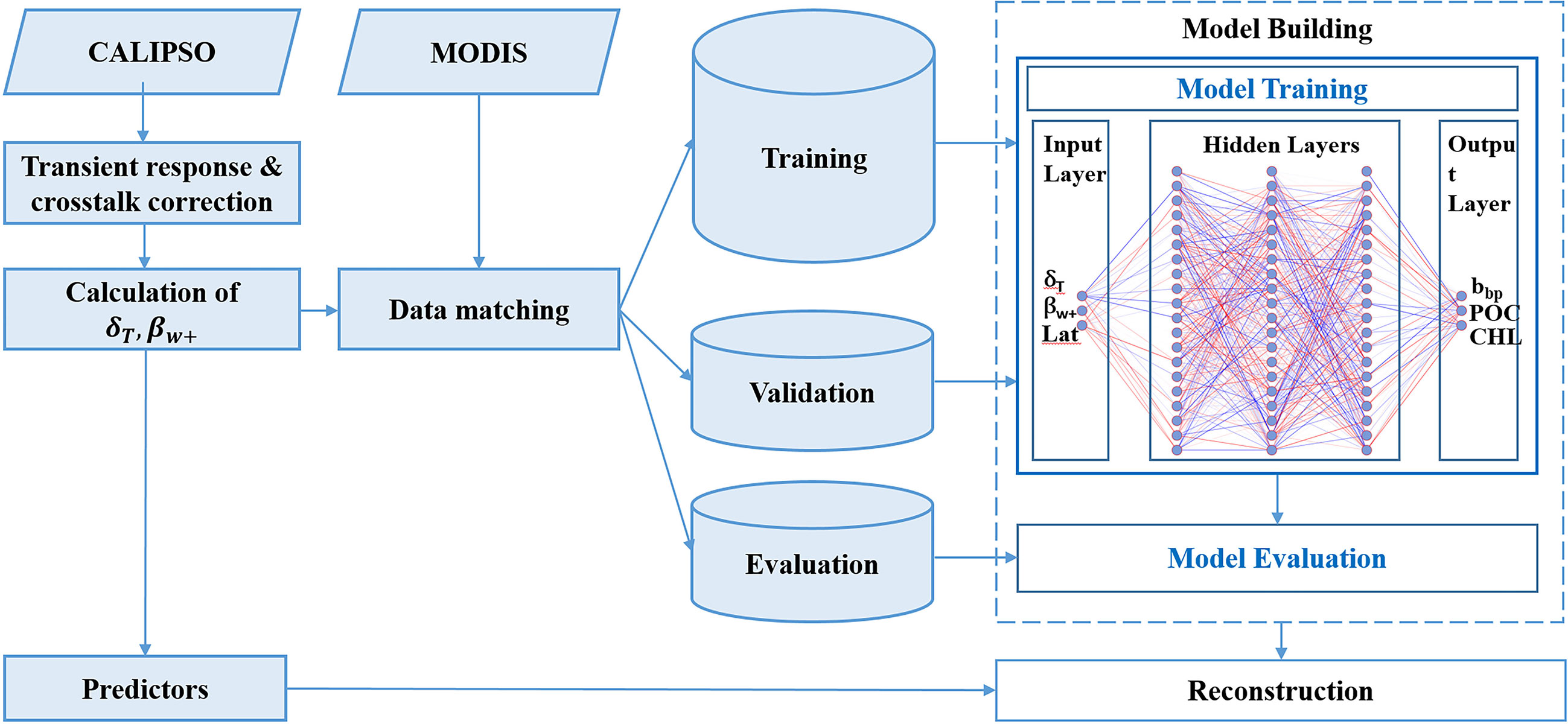
Figure 1 Flow chart of the FFNN including its architecture.

2.2.3 Evaluation metrics

Coefficient of determination (R²), root mean square error (RMSE), bias, mean absolute (MAE), and mean absolute percentage error (MAPE) are used to evaluate the results as follows:

where x_i is the true value, y_i is the prediction, f_i is the linear regression of y_i, and $\overline{y}$ is mean of y_i.

Linear correlation coefficient (r) is calculated to measure the strength of the linear relationship between phytoplankton parameters (Y) and marine environmental factors (X) as follows:

where σ is the standard deviation of variables and cov(*)is their covariance.

3 Results

3.1 FFNN training results and model evaluation

The training process including the decreases in losses and increases in R² is shown in Figure 2. An early stopping callback was used when the losses of the model used for validation data are no longer reduced. The early stopping callback could avoid overfitting effectively. Generally, the R² of the validation data for bbp, POC, and Chl could be around 0.8. The evaluation of the model is shown in Figure 3. The subset of data used for evaluation did not participate in the training. Therefore, the evaluation data represented independent observations. The RMSE and R² of bbp are 0.0011 m^-1 and 0.75, respectively. The RMSE and R² of POC are 36.74 mg/m³ and 0.82, respectively. The RMSE and R² of Chl are 1.3 mg/m³ and 0.84, respectively. Overall, the FFNN results have a good agreement with MODIS products.

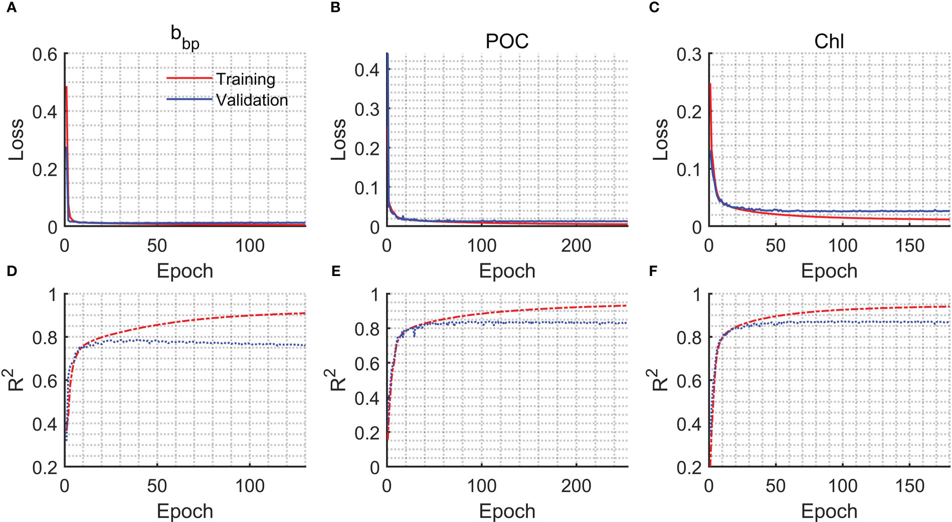
Figure 2 Loss and R2 versus epoch during the model training. (A) Loss of bbp, (B) loss of POC, (C) loss of Chl, (D) R2 of bbp, (E) R2 of POC, and (F) R2 of Chl.

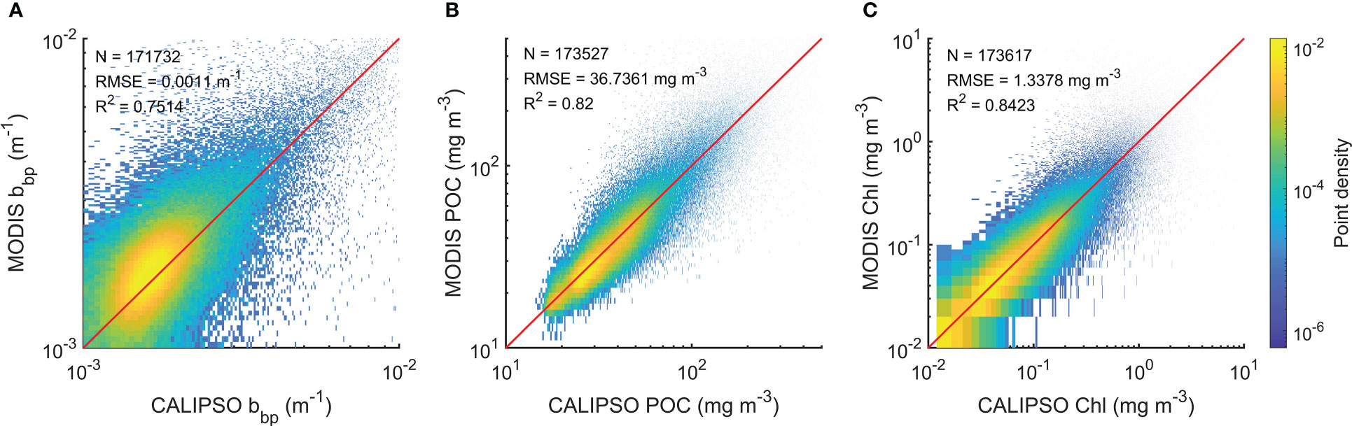
Figure 3 Evaluation of FFNN model. (A) Evaluation of bbp, (B) evaluation of POC, and (C) evaluation of Chl.

Figure 4 shows the spatial distribution of climatologically averaged CALIOP bbp and MODIS bbp in polar regions in summer (the Arctic in June, July, and August; the Antarctic in December, January, and February) from 2009 and 2021, which did not participate in the development of the model. The results of CALIOP have similar spatial distribution compared with MODIS products. The percent difference shown in Figures 4C, F is around 10%. Besides, the comparison with the Oregon State University (OSU) bbp data produced in previous studies (Behrenfeld et al., 2019), which can be downloaded from http://orca.science.oregonstate.edu/lidar_public_v2.php (accessed on 20 August 2022), is shown in Supplementary Figure 3. DNN-based CALIOP bbp have similar results and spatial distribution compared with previous studies in a global scale, but more details have been retained. The comparison of Chl between CALIOP and MODIS is shown in Figure 5. The difference in the Antarctic is slightly greater than that in the Arctic. But the percent difference is less than 25% shown in Figure 5F. The similar spatial distribution of POC between CALIOP and POC can be found in Figure 6. The results indicate that the FFNN method is effective for bbp, Chl, and POC inversion.

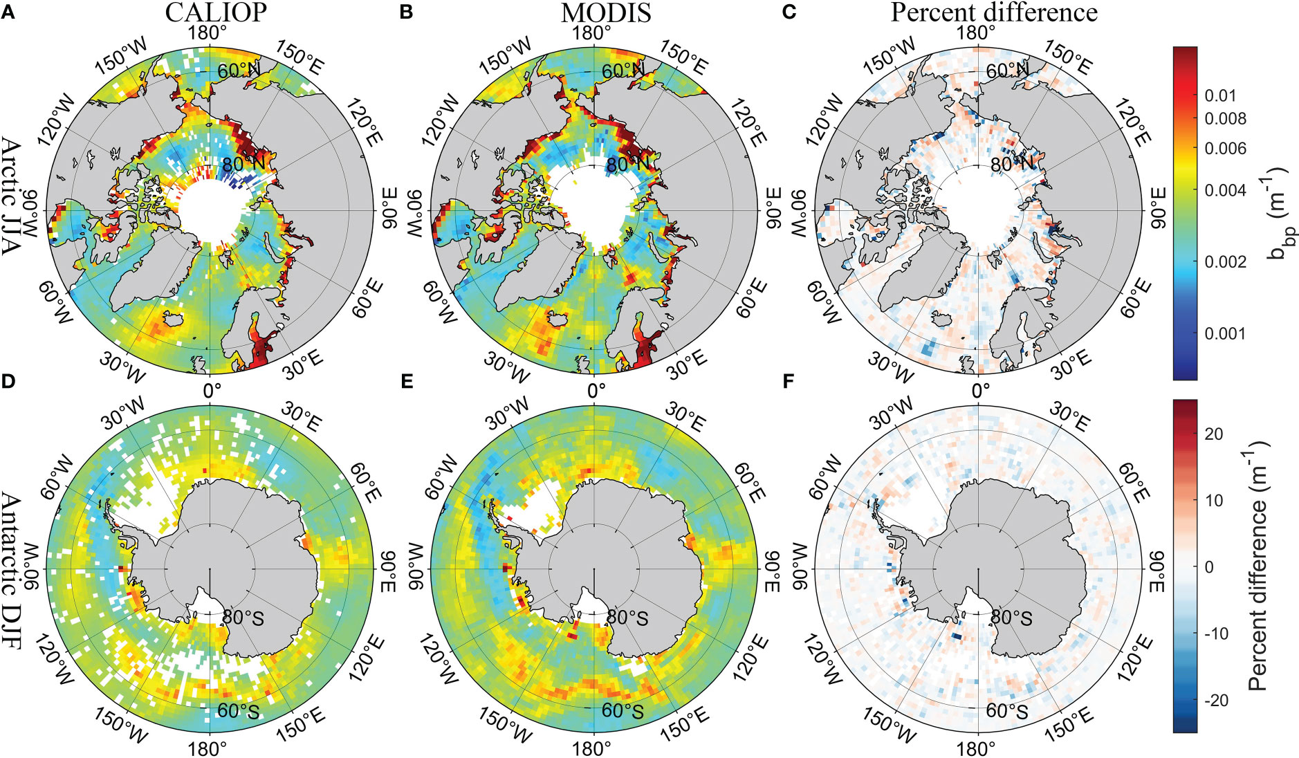
Figure 4 Comparisons of seasonal CALIOP bbp with MODIS bbp in polar regions in summer. (A) CALIOP bbp in the Arctic, (B) MODIS bbp in the Arctic, (C) percent difference between CALIOP bbp and MODIS bbp in the Arctic, (D) CALIOP bbp in the Antarctic, (E) MODIS bbp in the Antarctic, and (F) percent difference between CALIOP bbp and MODIS bbp in the Antarctic.

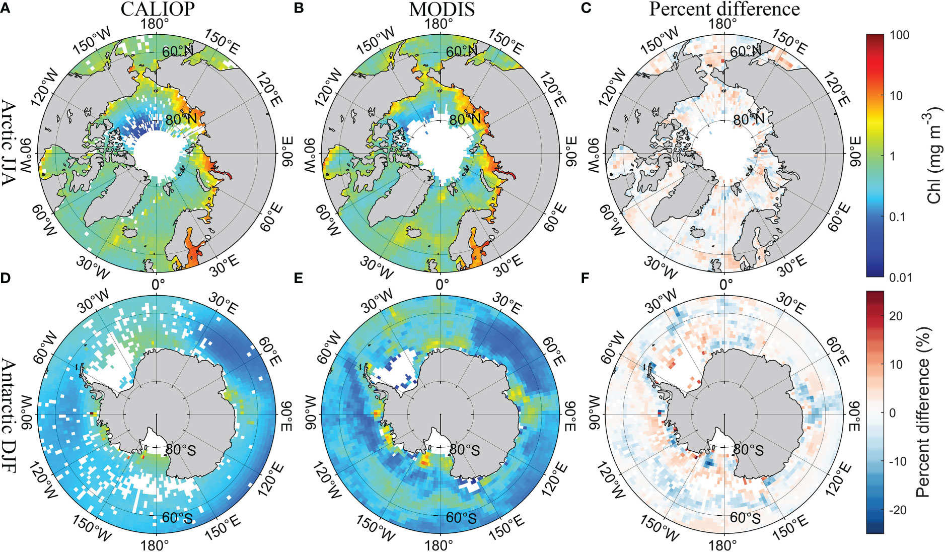
Figure 5 Comparisons of seasonal CALIOP Chl with MODIS Chl in polar regions in summer. (A) CALIOP Chl in the Arctic, (B) MODIS Chl in the Arctic, (C) percent difference between CALIOP Chl and MODIS Chl in the Arctic, (D) CALIOP Chl in the Antarctic, (E) MODIS Chl in the Antarctic, and (F) percent difference between CALIOP Chl and MODIS Chl in the Antarctic.

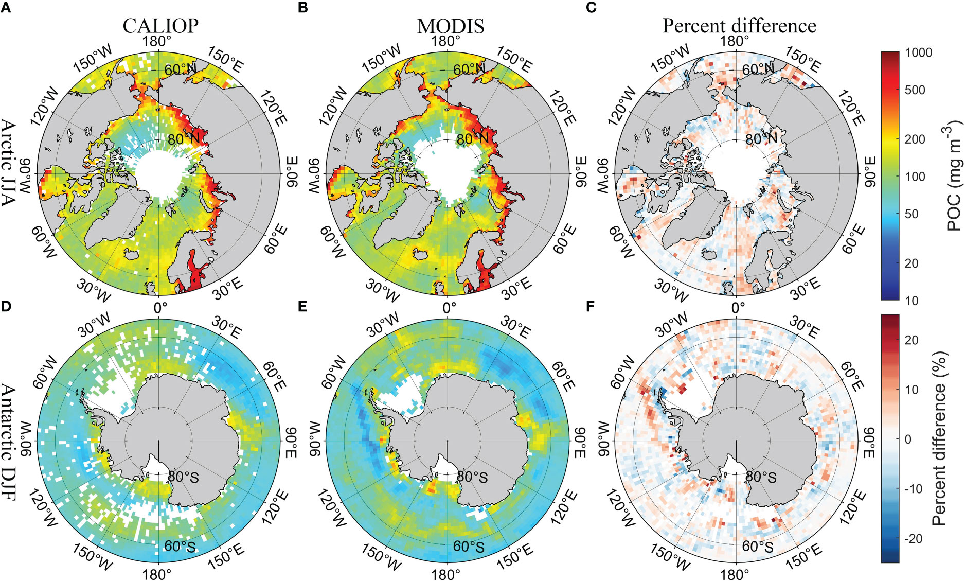
Figure 6 Comparisons of seasonal CALIOP POC with MODIS POC in polar regions in summer. (A) CALIOP POC in the Arctic, (B) MODIS POC in the Arctic, (C) percent difference between CALIOP POC and MODIS POC in the Arctic, (D) CALIOP POC in the Antarctic, (E) MODIS POC in the Antarctic, and (F) percent difference between CALIOP POC and MODIS POC in the Antarctic.

Figure 7 shows the data distribution in winter (the Arctic in December; the Antarctic in June). The deep blue represents the sea ice and the green color represents the distribution of Chl. It is clear that MODIS has poor coverage in polar regions in winter. Oppositely, CALIOP can observe high-latitude ocean areas even during lengthy polar nights. Therefore, CALIOP measurements can be a useful technique to study the phytoplankton and POC in polar areas.

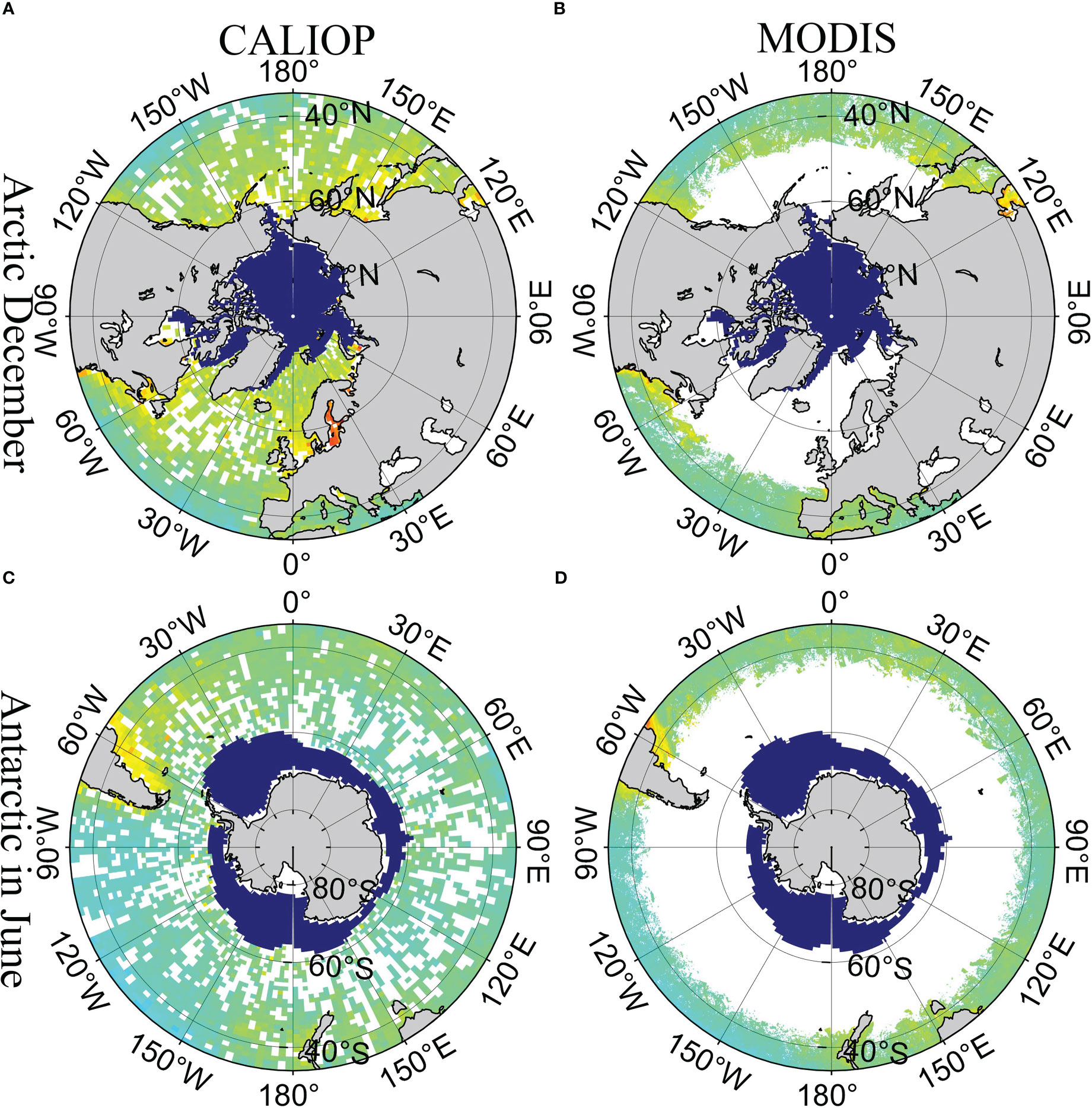
Figure 7 Distribution of CALIOP and MODIS in polar region in winter. (A) CALIOP data in the Arctic in December, (B) MODIS data in the Arctic in December, (C) CALIOP data in the Antarctic in June, and (D) MODIS data in the Antarctic in June. The deep blue represents the sea ice. The green color represents the Chl.

3.2 In situ validation

Figure 8 shows the matched data between Argo Chl and Chl derived from CALIOP and MODIS from 2010 to 2021. The data are matched if they fall within 9 km and occur within 12 hours of each other. The blue and red circles in Figure 8 represent the matched data point of CALIOP and MODIS, respectively. Dashed lines represent the best-fit functions and a green solid line represents the 1:1 line. There are 134 matched points in total and they are distributed around the green line. As shown in Table 1, R², RMSE, MAE, and MAPE between CALIOP and Argo are 0.5153, 0.6740, 0.5342, and 42.17%. The corresponding values of MODIS is 0.5902, 0.6379, 0.5150 and 38.82%. The biases of MODIS and CALIOP are 0.0972 and 0.0549, respectively. The Chl derived from CALIOP and MODIS agrees with the in situ measurements. The similar metrics with previous studies (Marrari et al., 2006; Moore et al., 2009; Hu et al., 2012; Moutier et al., 2019) indicate the FFNN algorithm can be used for retrieval of Chl from CALIOP.

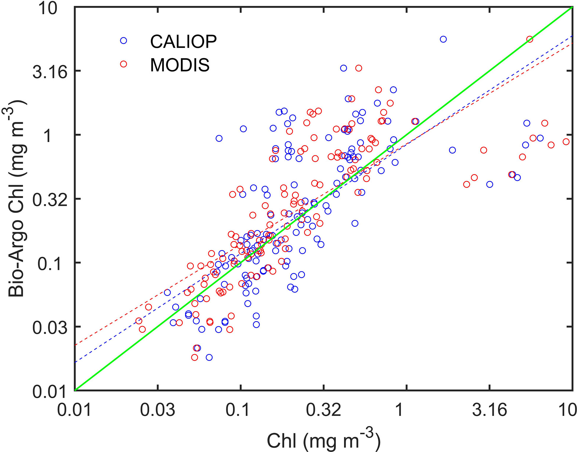
Figure 8 Matched data between Argo Chl and Chl produced by CALIOP and MODIS. The blue and red circles represent the matched data point of CALIOP and MODIS, respectively. Dashed lines represent the best-fit functions and a green solid line represents the 1:1 line.

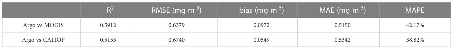
Table 1 Statistical analysis results of in situ Chl and remote sensing measurements.

3.3 Interannual variability

A spatial average of month Chl, bbp, and POC in polar regions has been performed to assess interannual variability. A large interannual variability and an apparent seasonal cycle in the average values can be found in Figure 9. In Arctic areas, Chl, bbp, and POC usually begin to increase in January and reach the maximum in summer. After that, the values begin to decrease. In Antarctic areas, Chl, bbp, and POC usually reach the peak in winter (in the northern hemisphere) and then begin to decrease. For Chl and POC, the values in the Antarctic are generally smaller than the values in the Arctic. Even the maximum values in the Antarctic are still smaller than the minimum values in the Arctic. The results show that the Arctic region may have a more productive ecosystem, which is consistent with previous studies in which phytoplankton biomass in north polar zone is much greater than that in south polar zone (Behrenfeld et al., 2017) Besides, some previous studies show that Chl in Arctic ocean is greater than that in Southern Ocean (Lewis et al., 2016; Behera et al., 2020).as well. For bbp, there are usually two peaks in Arctic areas as shown in Figure 9B. The first peak is usually the maximum and occurs in July. The second peak is smaller and occurs in October. The specific month in which the Chl concentration, bbp, and POC reach the maximum values each year is shown in Figure 10. The maximum in the Antarctic occurs at a more concentrated time, usually in winter (north hemisphere), more specifically, in January. The time may shift to December or February in some years. The month in which the maximum of Chl concentration, bbp, and POC occurs is more consistent. However, the results in the Arctic are more complicated. The maximum can occur in any month from May to October, not just in summer. In some years such as 2007, 2019, and 2020, Chl, bbp, and POC can reach their maximum simultaneously. But in some years, the months in which maximum values occur are different. For example, the bbp reached its peak in June 2014. Then, the Chl reached its maximum in July subsequently and the maximum of POC occurred in August at last. The results show that there is a certain connection between Chl, bbp, and POC, but there are some subtle differences between them.

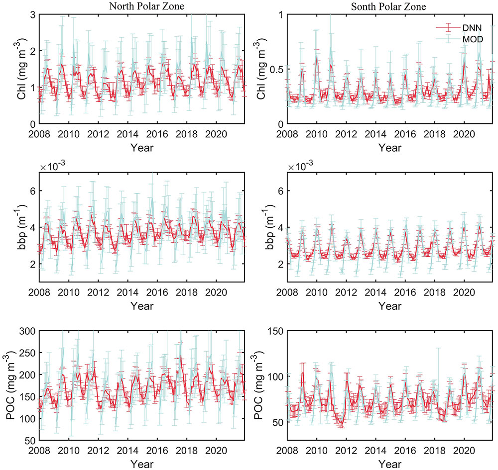
Figure 9 (Top) CALIOP-derived Chl spatial average in polar regions during 2007-2021. (Middle) bbp average in polar regions. (Bottom) POC average in polar regions.

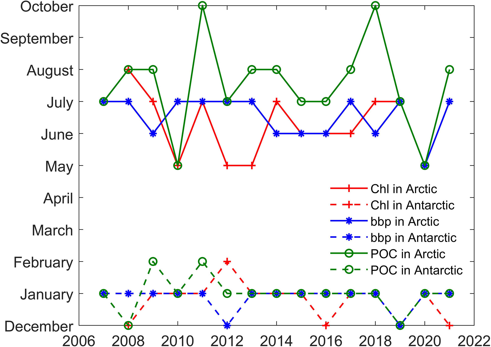
Figure 10 Month in which the Chl concentration, bbp, and POC reach the maximum values each year.

4 Discussion

The monthly change rate defined as dx_m = x_m−x_m−1 is calculated for Chl, bbp, and POC as shown in Figure 11, where m represents month. In the north polar region, the change rates of Chl and bbp usually become greater than zero from early spring when phytoplankton begin to grow. This may be caused by the combination of several factors. As shown in Figure 12, at this time the ice begins to melt, SST and PAR begin to rise, and MLD shoals. In May, the change rates of Chl and bbp reach the maximum, which indicates that phytoplankton reproduces rapidly. This may be caused by the proper PAR and SST as shown in Figure 12. The change rates of Chl and bbp usually start below zero in August, indicating the decline of phytoplankton. This is likely caused by the grazing of predators (Behrenfeld et al., 2017). The change rate of POC is much more complicated. There is no fixed month in which the change rate of POC reaches its peaks and it varies dramatically from year to year. This is related to the fluctuation of POC in the summer as shown in Figure 9. The change rate of Chl in the south polar region is much smaller than those in the north. This is largely because the prevalence of iron-limiting conditions constrains phytoplankton growth (de Baar, 2005; Boyd et al., 2007). As a result, the Chl and POC in the south are far lower than the values in the north. Table 2 shows the linear regression coefficient between bbp, Chl, POC, and environmental parameters. Note that all of the p values are less than 0.001, meaning that Chl, bbp, and POC are correlated with the SIE, PAR, SST, and MLD. But the impacts are different. It can be found that SIE and MLD have a negative impact on bbp, Chl, and POC. In terms of Chl, since the PAR has the highest correlation coefficient, it seems that phytoplankton is more affected by the light in polar areas. In fact, phytoplankton is often light-limited at higher latitudes (Riebesell et al., 2009). MLD likely has a great influence on bbp and the influence on POC of SIE in the Arctic is much greater than that in the Antarctic. The results indicate that environmentally driven factors of phytoplankton vary interannually at each pole (Behrenfeld et al., 2017).

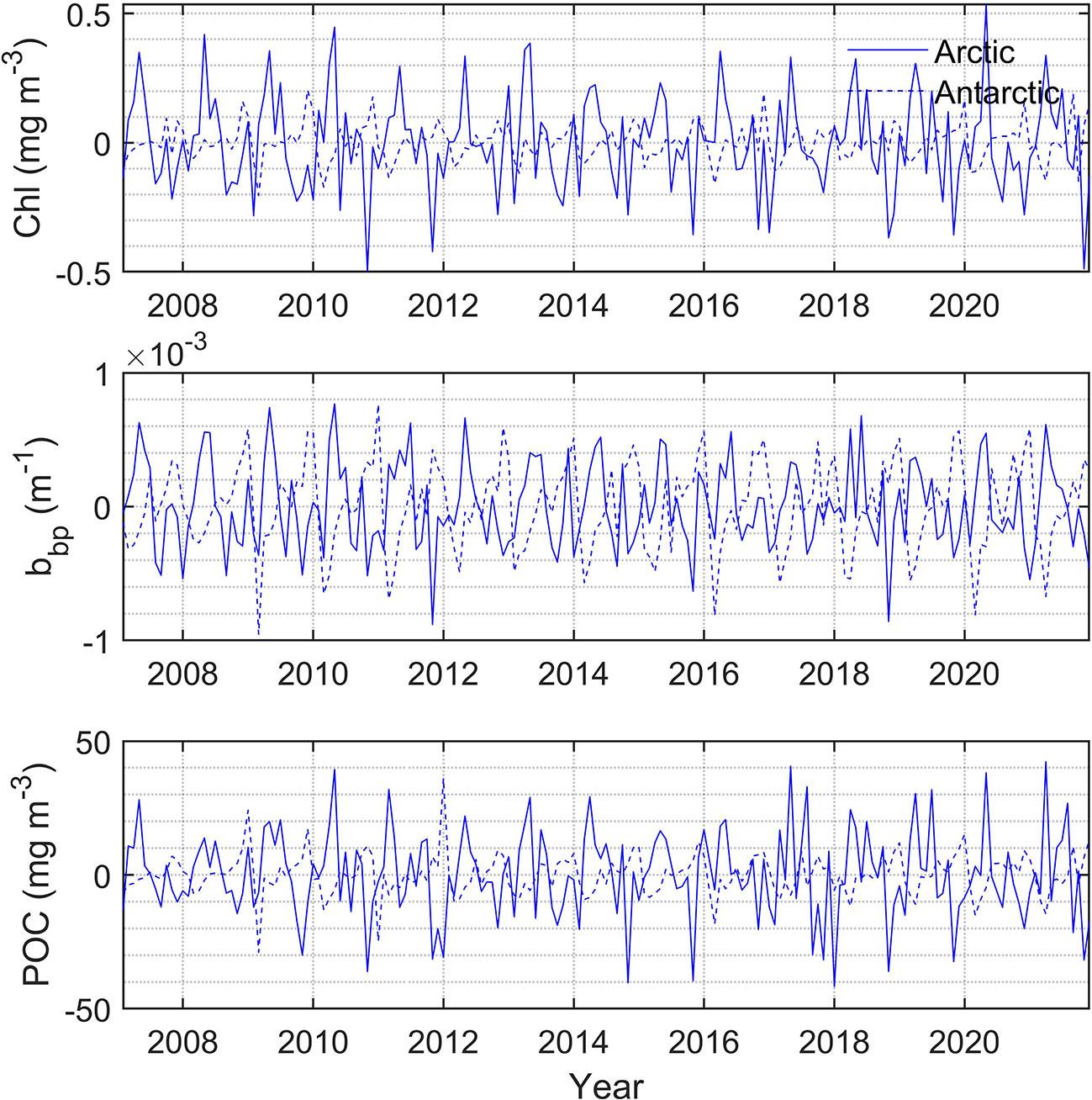
Figure 11 (Top) Chl change rate in polar regions during 2007-2021. (Middle) bbp change rate in polar regions. (Bottom) POC change rate in polar regions.

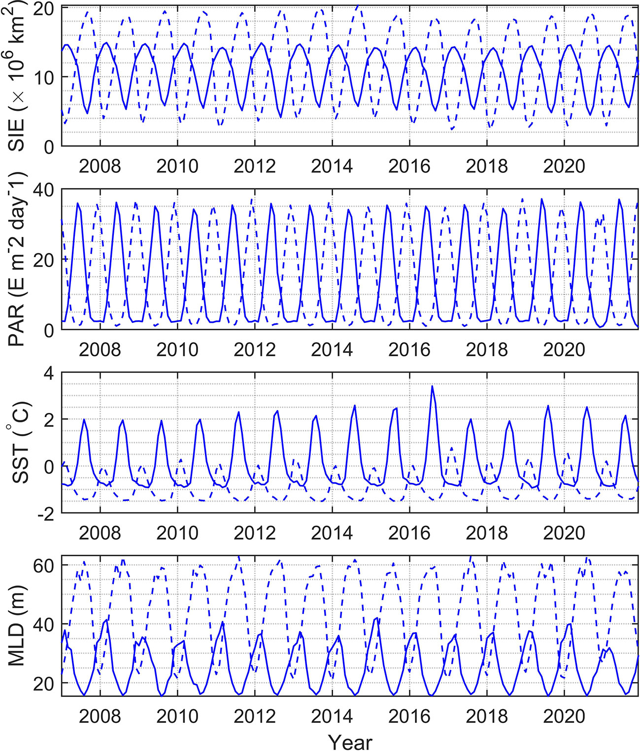
Figure 12 Spatial average of SIE, PAR, SST, and MLD in polar regions during 2007-2021. Solid and dashed lines represent the north and south polar zones, respectively.

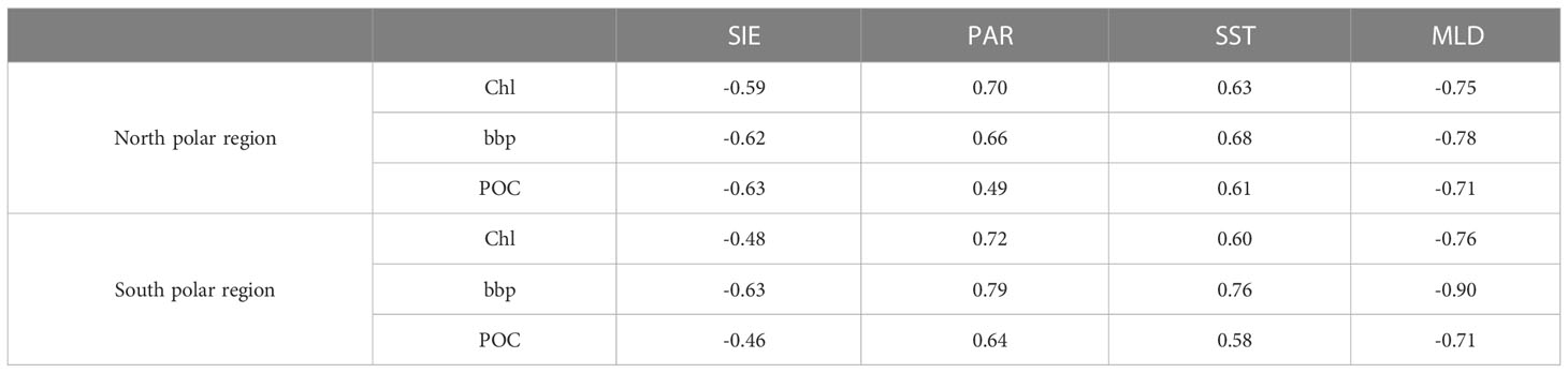
Table 2 Linear correlation coefficient between monthly average Chl, bbp, POC, and SIE, PAR, SST, MLD (N=178).

The monthly climatological averages of Chl, bbp, POC, SIE, PAR, SST, and MLD and their corresponding change rate are shown in Figure 13. In the north polar zone, Chl, bbp, and POC begin to increase in March, after they have reached their minimum in February. In March, SIE is still increasing and reaches its maximum. The result shows that the phytoplankton blooms before the sea ice starts melting in Arctic areas. SST barely changes at this time. But PAR increases a lot in Match. Therefore, the growth of phytoplankton in spring may be largely triggered by the increase of PAR. The change rates of Chl, bbp, and POC have the maximum in May, which indicates phytoplankton blooms. Meanwhile, PAR has the largest change rate in May as well. MLD has the smallest change rate meaning that MLD shoals rapidly at this time. Then, Chl and bbp reach the peak in July and begin to decline in August subsequently. POC is still increasing in August and reaches its peak at this time. In the south polar zone, Chl, bbp, and POC begin to increase in August when SIE is still increasing and SST is still decreasing. PAR begins to increase. Then Chl, bbp, and POC reach their maximums in January simultaneously. It can be found that Chl, bbp, and POC have a stronger correlation in Antarctic areas compared with Arctic areas. The results indicate that Chl, bbp, and POC have similar interannual variability but there are some subtle differences between them.

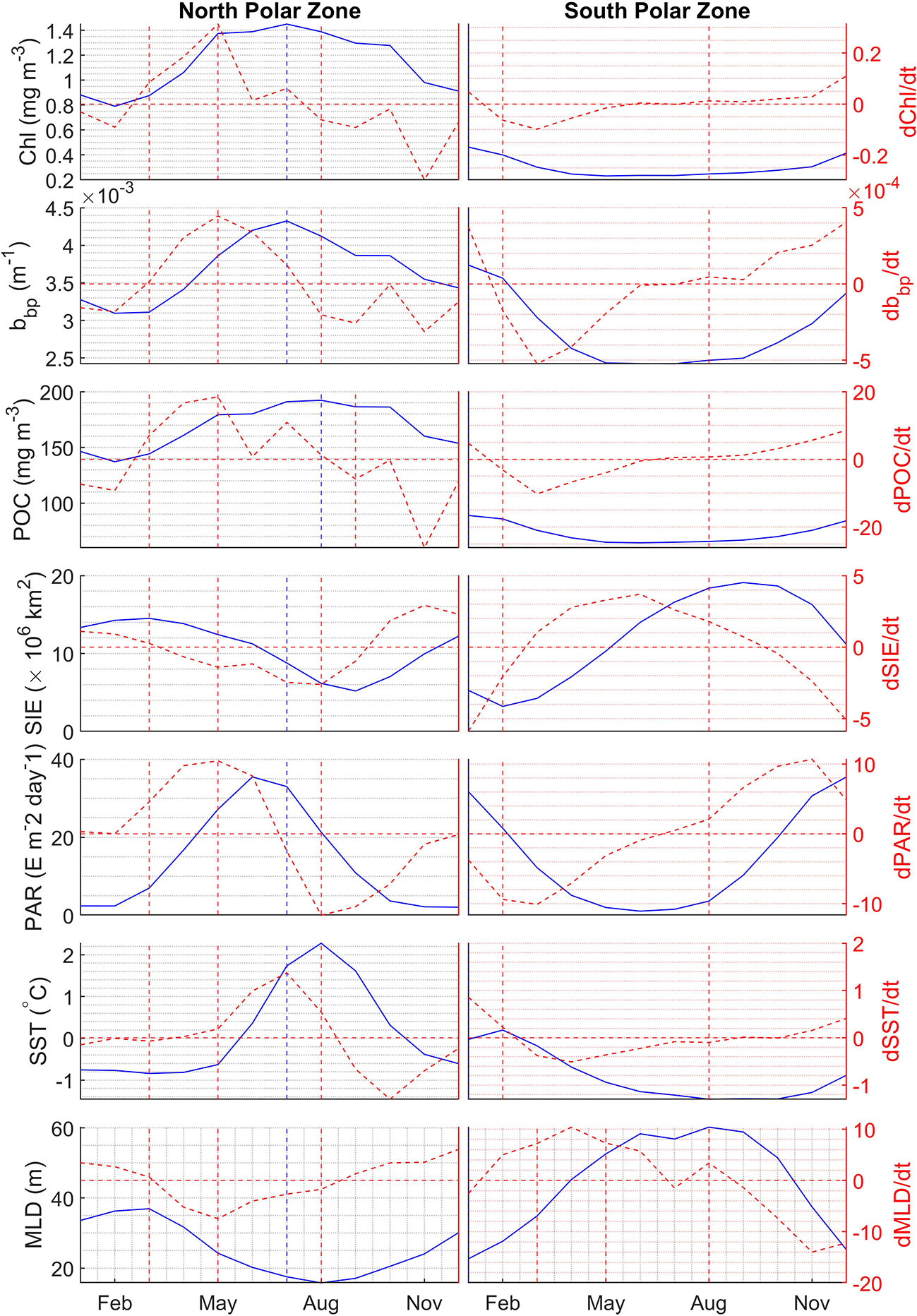
Figure 13 Monthly climatological average of Chl, bbp, POC, SIE, PAR, SST, and MLD represented by the blue solid lines, and their corresponding change rate represented by red dashed lines in the north polar zone (left panel) and south polar zone (right panel). Vertical lines represent the maximum values and the turning point when values begin to reduce or increase.

The total uncertainty (E) of DNN products can be expressed as the root of the squared sum of uncertainties stemming from measurement (M), representation (R), and prediction (P) errors: $E=\sqrt{M^2+R^2+P^2}$ (Gregor and Gruber, 2021). The measurement error includes the potential biases from the measurement MODIS and CALIOP data. The uncertainties of CALIOP δ_T and β;w₊ are about 1% and 10%, respectively(Lu et al., 2014). The uncertainty of MODIS bbp is approximately 30% (Bisson et al., 2019). The uncertainty of MODIS Chl is approximately 35% (Moore et al., 2009). The uncertainty of MODIS POC is approximately 25% (Evers-King et al., 2017). Therefore, the measurement errors of CALIOP-based bbp, Chl and POC are 32%, 36% and 27%, respectively. As the result of the fact that we developed the DNN model on a grid that is in many places coarser in time and space than the typical scales of variabilities of MODIS, the representation error is commonly assumed to be normally distributed with a bias of 0 on a global average (Gregor and Gruber, 2021). The prediction error is approximately 18% according to the validation data. Overall, the total uncertainties of CALIOP-based bbp, Chl and POC are 37%, 40% and 32%, respectively.

5 Conclusions

We proposed a new FFNN model for the retrieval of bbp, Chl, and POC from CALIOP. This data-based approach does not require additional assumptions regarding the relationship between b_bp and b(π). The FFNN is trained using the CALIPSO total ocean column-integrated depolarization ratio and subsurface column-integrated perpendicular backscatter together with collocated MODIS products. Non-linear relationship between lidar signal and bio-optical parameters was estimated through FFNN. Validation with independent data between CALIOP and MODIS with RMSE and R² of bbp are 0.0011 m^-1 and 0.75, those of POC are 36.7 mg/m³ and 0.82, and those of Chl are 1.3 mg/m³ and 0.84, indicates that the retrieval results agree well with MODIS products and in-situ BGC-Argo data. In order to assess the model further, it was compared to in situ Argo Chl with R², RMSE, MAE, and MAPE between CALIOP and Argo are 0.5153, 0.6740, 0.5342, and 42.17%, which demonstrates the effectiveness of the model. The performance of CALIOP product is close to MODIS after comparing it with Argo data. A merge product derived by combined active and passive remote sensing data could have a greater coverage and the algorithm used for the merge product will be further studied in the future to improve and produce the merge product.

Apparent seasonal cycles of phytoplankton can be observed. It was found that Chl, bbp, and POC have similar interannual variability but there are some subtle differences between them. Chl, bbp, and POC have a stronger correlation in Antarctic areas compared with Arctic areas. The combined analysis of bbp, Chl, and POC contributes to a comprehensive understanding of interannual variability in the ecosystem in polar regions. The coincidence of phytoplankton changes with PAR and the high linear regression coefficient indicates that sunlight is one key factor governing phytoplankton growth in polar regions. Future work should address the spatial variation of phytoplankton in polar regions.

Data availability statement

The original contributions presented in the study are included in the article/Supplementary Material. Further inquiries can be directed to the corresponding author.

Author contributions

ZZ: Conceptualization, Realization, and Writing-Original draft. PC: Supervision, Methodology, Reviewing. CX: Validation, Editing. CZ: Reviewing and Editing. MS: Validation and Editing. SZ: Editing. SC: Editing. DW: Editing. All authors contributed to the article and approved the submitted version.

Funding

National Key Research and Development Program of China (2022YFB3901703). This research was funded by the Key Special Project for Introduced Talents Team of Southern Marine Science and Engineering Guangdong Laboratory (GML2021GD0809), the National Natural Science Foundation (42276180; 41901305; 61991453), and the Key Research and Development Program of Zhejiang Province (2020C03100).

Acknowledgments

The authors gratefully acknowledge the NASA Langley Research Center for providing CALIOP data through the Atmospheric Science Data Center (https://asdc.larc.nasa.gov/data/CALIPSO/). We are grateful to the NASA Ocean Biology Processing Group for providing MODIS products (https://oceandata.sci.gsfc.nasa.gov/) and biogeochemical-Argo data from the Argo Data Assembly Center (ftp://ftp.ifremer.fr/ifremer/argo/dac/). We thank the reviewers for their suggestions, which significantly improved the presentation of the paper.

Conflict of interest

The authors declare that the research was conducted in the absence of any commercial or financial relationships that could be construed as a potential conflict of interest.

Publisher’s note

All claims expressed in this article are solely those of the authors and do not necessarily represent those of their affiliated organizations, or those of the publisher, the editors and the reviewers. Any product that may be evaluated in this article, or claim that may be made by its manufacturer, is not guaranteed or endorsed by the publisher.

Supplementary material

The Supplementary Material for this article can be found online at: https://www.frontiersin.org/articles/10.3389/fmars.2023.1050087/full#supplementary-material

Supplementary Figure 1 | The spatial distribution of in situ data (A) and histograms of all data (B) and matched data (C).

Supplementary Figure 2 | Point density of the matched data. (A) training data; (B) validation data; (C) evaluation data.

Supplementary Figure 3 | Comparison between DNN-based CALIOP products with Oregon State University (OSU) CALIOP products in 2009. (A) DNN products (B) OSU products.

References

Alvera-Azcárate A., van der Zande D., Barth A., Troupin C., Martin S., Beckers J.-M. (2021). Analysis of 23 years of daily cloud-free chlorophyll and suspended particulate matter in the greater north Sea. Front. Mar. Sci. 8. doi: 10.3389/fmars.2021.707632
Behera N., Swain D., Sil S. (2020). Effect of Antarctic sea ice on chlorophyll concentration in the southern ocean. Deep Sea Res. Part II: Topical Stud. Oceanogr. 178, 104853. doi: 10.1016/j.dsr2.2020.104853
Behrenfeld M. J., Gaube P., Della Penna A., O'Malley R. T., Burt W. J., Hu Y., et al. (2019). Global satellite-observed daily vertical migrations of ocean animals. Nature 576 (7786), 257–261. doi: 10.1038/s41586-019-1796-9
Behrenfeld M. J., Hu Y., Hostetler C. A., Dall'Olmo G., Rodier S. D., Hair J. W., et al. (2013). Space-based lidar measurements of global ocean carbon stocks. Geophys. Res. Lett. 40 (16), 4355–4360. doi: 10.1002/grl.50816
Behrenfeld M. J., Hu Y., O’Malley R. T., Boss E. S., Hostetler C. A., Siegel D. A., et al. (2017). Annual boom–bust cycles of polar phytoplankton biomass revealed by space-based lidar. Nat. Geosci. 10 (2), 118–122. doi: 10.1038/ngeo2861
Bell B., Hersbach H., Simmons A., Berrisford P., Dahlgren P., Horányi A., et al. (2021). The ERA5 global reanalysis: Preliminary extension to 1950. Q. J. R. Meteorological Soc. 147 (741), 4186–4227. doi: 10.1002/qj.4174
Berthon J. F., Shybanov E., Lee E. G., Zibordi G. (2007). Measurements and modeling of the volume scattering function in the coastal northern Adriatic Sea. Appl. Optics 46 (22), 5189–5203. doi: 10.1364/AO.46.005189
Bisson K. M., Boss E., Werdell P. J., Ibrahim A., Behrenfeld M. J. (2021). Particulate backscattering in the global ocean: A comparison of independent assessments. Geophys. Res. Lett. 48 (2), e2020GL090909. doi: 10.1029/2020gl090909
Bisson K. M., Boss E., Westberry T. K., Behrenfeld M. J. (2019). Evaluating satellite estimates of particulate backscatter in the global open ocean using autonomous profiling floats. Opt Express 27 (21), 30191–30203. doi: 10.1364/OE.27.030191
Blondeau-Patissier D., Gower J. F. R., Dekker A. G., Phinn S. R., Brando V. E. (2014). A review of ocean color remote sensing methods and statistical techniques for the detection, mapping and analysis of phytoplankton blooms in coastal and open oceans. Prog. Oceanogr. 123, 123–144. doi: 10.1016/j.pocean.2013.12.008
Boss E., Pegau W.S.J.A.O. (2001). Relationship of light scattering at an angle in the backward direction to the backscattering coefficient. Applied Optics 40 (30), 5503–5507. doi: 10.1364/AO.40.005503
Boyd P. W., Jickells T., Law C. S., Blain S., Boyle E. A., Buesseler K. O., et al. (2007). Mesoscale iron enrichment experiments 1993-2005: synthesis and future directions. Science 315 (5812), 612–617. doi: 10.1126/science.1131669
Brewin R. J. W., Ciavatta S., Sathyendranath S., Jackson T., Tilstone G., Curran K., et al. (2017). Uncertainty in ocean-color estimates of chlorophyll for phytoplankton groups. Front. Mar. Sci. 4. doi: 10.3389/fmars.2017.0010
Capuzzo E., Lynam C. P., Barry J., Stephens D., Forster R. M., Greenwood N., et al. (2018). A decline in primary production in the north Sea over 25 years, associated with reductions in zooplankton abundance and fish stock recruitment. Glob Chang Biol. 24 (1), e352–e364. doi: 10.1111/gcb.13916
Chami M., Marken E., Stamnes J., Khomenko G., Korotaev G. (2006). Variability of the relationship between the particulate backscattering coefficient and the volume scattering function measured at fixed angles 111 (C5). doi: 10.1029/2005JC003230
Chami M., Thirouard A., Harmel T. (2014). POLVSM (Polarized volume scattering meter) instrument: an innovative device to measure the directional and polarized scattering properties of hydrosols. Optics Express 22 (21), 26403–26428. doi: 10.1364/OE.22.026403
Churnside J. H., Marchbanks R. D. (2015). Subsurface plankton layers in the Arctic ocean. Geophys. Res. Lett. 42 (12), 4896–4902. doi: 10.1002/2015gl064503
Churnside J. H., Sullivan J. M., Twardowski M. S. (2014). Lidar extinction-to-backscatter ratio of the ocean. Optics express 22 (15), 18698–18706. doi: 10.1364/OE.22.018698
Claustre H., Johnson K. S., Takeshita Y. (2019). Observing the global ocean with biogeochemical-argo. Annu. Rev. Mar. Sci. 12 (1), 23–48. doi: 10.1146/annurev-marine-010419-010956
de Baar H. J. W. (2005). Synthesis of iron fertilization experiments: From the iron age in the age of enlightenment. J. Geophys. Res. 110 (C9). doi: 10.1029/2004jc002601
Dickey T., Lewis M., Chang G. (2006). Optical oceanography: Recent advances and future directions using global remote sensing and in situ observations. Rev. Geophys. 44 (1). doi: 10.1029/2003RG000148
Dionisi D., Brando V. E., Volpe G., Colella S., Santoleri R. (2020). Seasonal distributions of ocean particulate optical properties from spaceborne lidar measurements in Mediterranean and black sea. Remote Sens. Environ. 247, 111889. doi: 10.1016/j.rse.2020.111889
Evers-King H., Martinez-Vicente V., Brewin R. J. W., Dall'Olmo G., Hickman A. E., Jackson T., et al. (2017). Validation and intercomparison of ocean color algorithms for estimating particulate organic carbon in the oceans. Front. Mar. Sci. 4. doi: 10.3389/fmars.2017.00251
Frouin R. J., Frouin R., McPherson J., Ueyoshi K., Franz B. A., Ebuchi N., et al. (2012). “A time series of photosynthetically available radiation at the ocean surface from SeaWiFS and MODIS data,” in Remote sensing of the marine environment II (Kyoto, Japan: Proc.SPIE).
Getzewich B. J., Vaughan M. A., Hunt W. H., Avery M. A., Powell K. A., Tackett J. L., et al. (2018). CALIPSO lidar calibration at 532 nm: version 4 daytime algorithm. Atmospheric Measurement Techniques 11 (11), 6309–6326. doi: 10.5194/amt-11-6309-2018
Gordon H. R., Clark D. K., Mueller J. L., Hovis W. A. (1980). Phytoplankton pigments from the nimbus-7 coastal zone color scanner: comparisons with surface measurements. Science 210 (4465), 63–66. doi: 10.1126/science.210.4465.63
Gregor L., Gruber N. (2021). OceanSODA-ETHZ: A global gridded data set of the surface ocean carbonate system for seasonal to decadal studies of ocean acidification. Earth System Sci. Data 13 (2), 777–808. doi: 10.5194/essd-13-777-2021
Hersbach H., Bell B., Berrisford P., Hirahara S., Horányi A., Muñoz-Sabater J., et al. (2020). The ERA5 global reanalysis. Q. J. R. Meteorological Soc. 146 (730), 1999–2049. doi: 10.1002/qj.3803
Hinton G., Srivastava N., Swersky K. (2012) Lecture 6a: Overview of mini-batch gradient descent, neural networks for machine learning, slides. Available at: http://www.cs.toronto.edu/~tijmen/csc321/slides/lecture_slides_lec6.pdf.
Hu C., Lee Z., Franz B. (2012). Chlorophyll a algorithms for oligotrophic oceans: A novel approach based on three-band reflectance difference. J. Geophys. Research: Oceans 117 (C1). doi: 10.1029/2011jc007395
Hu Y., Stamnes K., Vaughan M., Pelon J., Weimer C., Wu D., et al. (2008). Sea Surface wind speed estimation from space-based lidar measurements. Atmospheric Chem. Phys. Discussions 8 (1), 2771–2793. doi: 10.5194/acpd-8-2771-2008
Hu L., Zhang X., Xiong Y., Gray D. J., He M. X. (2020). Variability of relationship between the volume scattering function at 180° and the backscattering coefficient for aquatic particles. Appl. Optics 59 (10), C31–C41. doi: 10.1364/ao.383229
Jackson T., Sathyendranath S., Mélin F. (2017). An improved optical classification scheme for the ocean colour essential climate variable and its applications. Remote Sens. Environ. 203, 152–161. doi: 10.1016/j.rse.2017.03.036
Jamet C., Ibrahim A., Ahmad Z., Angelini F., Babin M., Behrenfeld M. J., et al. (2019). Going beyond standard ocean color observations: Lidar and polarimetry. Front. Mar. Sci. 6. doi: 10.3389/fmars.2019.00251
Kim M.-H., Kim S.-W., Yoon S.-C., Omar A. H. (2013). Comparison of aerosol optical depth between CALIOP and MODIS-aqua for CALIOP aerosol subtypes over the ocean. J. Geophys. Research: Atmospheres 118 (23), 13,241–213,252. doi: 10.1002/2013jd019527
Lee Z., Carder K. L., Arnone R. A. (2002). Deriving inherent optical properties from water color: a multiband quasi-analytical algorithm for optically deep waters. Appl. Optics 41 (27), 5755–5772. doi: 10.1364/AO.41.005755
Lee J. H., Churnside J. H., Marchbanks R. D., Donaghay P. L., Sullivan J. M. (2013). Oceanographic lidar profiles compared with estimates from in situ optical measurements. Appl. Optics 52 (4), 786–794. doi: 10.1364/AO.52.000786
Lewis K. M., Mitchell B. G., van Dijken G. L., Arrigo K. R. (2016). Regional chlorophyll a algorithms in the Arctic ocean and their effect on satellite-derived primary production estimates. Deep Sea Res. Part II: Topical Stud. Oceanogr. 130, 14–27. doi: 10.1016/j.dsr2.2016.04.020
Li X., Mao Z., Zheng H., Zhang W., Yuan D., Li Y., et al. (2022). Process-oriented estimation of chlorophyll-a vertical profile in the Mediterranean Sea using MODIS and oceanographic float products. Front. Mar. Sci. 9. doi: 10.3389/fmars.2022.933680
Lu X., Hu Y., Trepte C., Zeng S., Churnside J. H. (2014). Ocean subsurface studies with the CALIPSO spaceborne lidar. J. Geophys. Research: Oceans 119 (7), 4305–4317. doi: 10.1002/2014jc009970
Maritorena S., Siegel D. A., Peterson A. R. (2002). Optimization of a semianalytical ocean color model for global-scale applications. Appl. Optics 41 (15), 2705–2714. doi: 10.1364/AO.41.002705
Marrari M., Hu C., Daly K. (2006). Validation of SeaWiFS chlorophyll a concentrations in the southern ocean: A revisit. Remote Sens. Environ. 105 (4), 367–375. doi: 10.1016/j.rse.2006.07.008
McClain C. R. (2009). A decade of satellite ocean color observations. Annu. Rev. Mar. Sci. 1 (1), 19–42. doi: 10.1146/annurev.marine.010908.163650
Moore T. S., Campbell J. W., Dowell M. D. (2009). A class-based approach to characterizing and mapping the uncertainty of the MODIS ocean chlorophyll product. Remote Sens. Environ. 113 (11), 2424–2430. doi: 10.1016/j.rse.2009.07.016
Moutier W., Thomalla S., Bernard S., Wind G., Ryan-Keogh T., Smith M. (2019). Evaluation of chlorophyll-a and POC MODIS aqua products in the southern ocean. Remote Sens. 11 (15), 1793. doi: 10.3390/rs11151793
Murphy A., Hu Y. (2021). Retrieving aerosol optical depth and high spatial resolution ocean surface wind speed from CALIPSO: A neural network approach. Front. Remote Sens. 1. doi: 10.3389/frsen.2020.614029
O'Reilly J. E., Maritorena S., Mitchell B. G., Siegel D. A., Carder K. L., Garver S. A., et al. (1998). Ocean color chlorophyll algorithms for SeaWiFS. J. Geophys. Research: Oceans 103 (C11), 24937–24953. doi: 10.1029/98jc02160
Parekh P., Dutkiewicz S., Follows M. J., Ito T. (2006). Atmospheric carbon dioxide in a less dusty world. Geophys. Res. Lett. 33 (3). doi: 10.1029/2005gl025098
Riebesell U., Kortzinger A., Oschlies A. (2009). Sensitivities of marine carbon fluxes to ocean change. Proc. Natl. Acad. Sci. U.S.A. 106 (49), 20602–20609. doi: 10.1073/pnas.0813291106
Sharma S., Sharma S., Athaiya A. (2020). Activation functions in neural networks. Int. J. Eng. Appl. Sci. Technol. 4 (12), 310–316.
Stramski D., Reynolds R. A., Babin M., Kaczmarek S., Lewis M. R., Röttgers R., et al. (2008). Relationships between the surface concentration of particulate organic carbon and optical properties in the eastern south pacific and eastern Atlantic oceans. Biogeosciences 5 (1), 171–201. doi: 10.5194/bg-5-171-2008
Sullivan J. M., Twardowski M. S. (2009). Angular shape of the oceanic particulate volume scattering function in the backward direction. Appl. Optics 48 (35), 6811–6819. doi: 10.1364/AO.48.006811
Werdell P. J., Franz B. A., Bailey S. W., Feldman G. C., Boss E., Brando V. E., et al. (2013). Generalized ocean color inversion model for retrieving marine inherent optical properties. Appl. Optics 52 (10), 2019–2037. doi: 10.1364/AO.52.002019
Whitmire A. L., Pegau W. S., Karp-Boss L., Boss E., Cowles T. J. (2010). Spectral backscattering properties of marine phytoplankton cultures 18 (14), 15073–15093. doi: 10.1364/OE.18.015073
Winker D. M., Vaughan M. A., Omar A., Hu Y., Powell K. A., Liu Z., et al. (2009). Overview of the CALIPSO mission and CALIOP data processing algorithms. J. Atmospheric Oceanic Technol. 26 (11), 2310–2323. doi: 10.1175/2009jtecha1281.1
Xu X., Lemmen C., Wirtz K. W. (2020). Less nutrients but more phytoplankton: Long-term ecosystem dynamics of the southern north Sea. Front. Mar. Sci. 7. doi: 10.3389/fmars.2020.00662
Zhang X., Boss E., Gray D. J. (2014). Significance of scattering by oceanic particles at angles around 120 degree 22 (25) 31329–31336. doi: 10.1364/OE.22.031329
Keywords: chlorophyll, bbp, POC, CALIOP, polar oceans, phytoplankton
Citation: Zhang Z, Chen P, Zhong C, Xie C, Sun M, Zhang S, Chen S and Wu D (2023) Chlorophyll and POC in polar regions derived from spaceborne lidar. Front. Mar. Sci. 10:1050087. doi: 10.3389/fmars.2023.1050087
Received: 21 September 2022; Accepted: 23 January 2023;
Published: 03 February 2023.
Edited by:
Javier A. Concha, European Space Research Institute (ESRIN), ItalyReviewed by:
Shengqiang Wang, Nanjing University of Information Science and Technology, ChinaYongxiang Hu, Langley Research Center (NASA), United States
Copyright © 2023 Zhang, Chen, Zhong, Xie, Sun, Zhang, Chen and Wu. This is an open-access article distributed under the terms of the Creative Commons Attribution License (CC BY). The use, distribution or reproduction in other forums is permitted, provided the original author(s) and the copyright owner(s) are credited and that the original publication in this journal is cited, in accordance with accepted academic practice. No use, distribution or reproduction is permitted which does not comply with these terms.
*Correspondence: Peng Chen, chenp@sio.org.cn