Dynamical interactions between Loop Current and Loop Current Frontal Eddies in a HYCOM ensemble of the circulation in the Gulf of Mexico

1 Introduction

The Loop Current (LC) dominates the oceanic flow in the Gulf of Mexico (GoM) as it is its most energetic feature. The LC enters the Gulf through the Yucatan Channel and exits through the Florida Straits before it becomes the Gulf Stream. The path of the LC is highly variable. It can flow directly from the Yucatan Channel to the Florida Straits, which is usually referred to as the ‘port to port’ state (Schmitz, 2005). The LC can also have an extended state when its northern tip intrudes northward into the eastern GoM basin. The extended state LC sheds an anticyclonic LC eddy (LCE) intermittently at irregular intervals (Schmitz, 2003). The LCEs may re-attach to and detach from the LC several times before the final detachment (Schmitz, 2005). After the final detachment, the LCE propagates westwards, and the LC retreats depending on the size of the detached LCE (Leben, 2005).

Given its dynamic and highly variable nature, understanding the LC system’s dynamics is vital for improving the LC circulation forecasts in the GoM, and thereby providing valuable information for marine operations in the GoM such as: pollutant transport (Walker et al., 2011; Le Hénaff et al., 2012b), hurricane intensification (Bao et al., 2000; Jaimes et al., 2006), and oil platform operations (National Academies of Sciences et al., 2018). The dynamical processes and mechanisms involved in LCE sheddings have been the subject of many observational, theoretical and modeling studies. Modeling studies reveal that both baroclinic and barotropic instabilities play roles in the separation process of LCEs (Hurlburt and Thompson, 1982; Cherubin et al., 2005). Pichevin and Nof (1997) proposed the momentum imbalance paradox for explaining eddy separation. Analysis of the observations from the CANEK program (Candela et al., 2002) revealed that potential vorticity (PV) flux anomaly at the Yucatan Channel may serve as a useful indicator of Loop Current variability, including Loop Current extension, retraction, and eddy shedding (Candela et al., 2003; Oey, 2004). A nearly linear relationship between the Loop Current retreat latitude and the subsequent separation period was found via altimeter-derived LC metrics (Leben, 2005). By analyzing hydrographic data, Sturges and Evans (1983) indicated that the north-south fluctuations in the Loop Current position are correlated with the sea level at the coast and presumably with coastal currents. Deep eddies and deep flows are found to influence the LCE shedding process as well (Oey, 2008; Chang and Oey, 2011). Observational data has also linked LCE detachments to eddies or perturbations coming from the Caribbean Sea (Athié et al., 2012; Androulidakis et al., 2021; Le Hénaff et al., 2023; Ntaganou et al., 2023) and pulses of increased transport through the Florida Straits (Sturges et al., 2010).

Previous studies have revealed the important roles that the Loop Current Frontal Eddies (LCFEs) play in the LC dynamics and its detachment. The observation of these cold, cyclonic eddies along the LC edge was first documented by Cochrane (1972). Vukovich & Maul (1985) found that, on the eastern side of the LC, LCFEs have diameters in the range of 80–120 km and reach at least 1000 m depth. According to the authors, these eddies can move westward and lead to an LCE detachment or separation. Fratantoni et al. (1998) used Sea Surface Temperature (SST) satellite data to reveal that a cyclonic eddy would stay longer near the Dry Tortugas when an LCE is shed. Zavala-Hidalgo et al. (2003) investigated cyclonic eddies over the northeast Campeche Bank (CB) and documented their formation and life cycle (either their decay or their north/northwest migration). They noted in particular that their formation coincides with LCE detachments. The LCE detachment types were categorized into two general modes by Schmitz (2005). One is primarily due to pinch-off by cyclones on the boundary of the LC, the other when the LC is being pulled apart by the westward propagation of its own tip. The numerical simulations of Androulidakis et al. (2014) confirmed the role of northern LCFE and CB LCFE in necking down the LC during LCE detachment.In addition, the bathymetry of the Mississippi Fan was found to play a role in intensifying LCFEs along the extended LC northern edge (Le Hénaff et al., 2012a). In their analysis of mooring data in both the northeast and southeast GoM, Hamilton et al. (2016) found that the steepening of the LC meanders leads to a pinch-off of LC eddies, and that the deep lower-layer eddies, constrained by the closed topography of the southeastern Gulf, appear to assist in achieving separation. Finally, Sheinbaum et al. (2016), using some of the same mooring observations, found that some LCE detachments are dominated by a cyclone associated with a meander through the southward flowing branch of the LC, e.g., Eddy Ekman and Eddy Franklin in 2010-2011, while during some other events (Eddy Cameron and Eddy Darwin in 2008-2009¹, the CB cyclone appears to be nearly as strong as the ones coming from the eastern side of the LC.

While previous studies have explored the dynamics of the LC system, including the LCFEs and LCEs, there are still gaps in our understanding of this system. Specifically, in ocean model simulations, the influence of initial condition perturbations, on the subsequent development of LCFEs and the detachment of LCEs remains underexplored. Furthermore, the existence of a teleconnection between distinct LCFEs, that is, a distant interaction between LCFEs that ring the LC system and propagate along its rim, has not been seriously studied, although this possibility was brought up by Schmitz (2005).

This study attempts to fill these gaps by applying targeted ensemble simulations to investigate the dynamics of the LC system during the shedding of Eddy Franklin in 2010 (see Figure 1), with a particular emphasis on the impact of initial condition perturbations on the development of LCFEs and the detachment of LCEs. In addition, the possible teleconnection between distinct LCFEs is statistically investigated. The realism of the model outputs is also evaluated by comparing ensemble simulations with mooring observations. This study is a continuation of the work in Iskandarani et al. (2016) and Wang et al. (2018), aiming to provide deeper insights into the LC system’s dynamics and its implications for the GoM circulation forecasts. The analysis herein shows that the initial condition perturbations have a significant impact on the LCE detachment and its timing, and that larger and stronger LCFEs are more likely to be followed by an LCE detachment. Moreover, when a large and strong LCFE intrudes into the LC from the east, a second LCFE on the western side of the LC is prone to form.

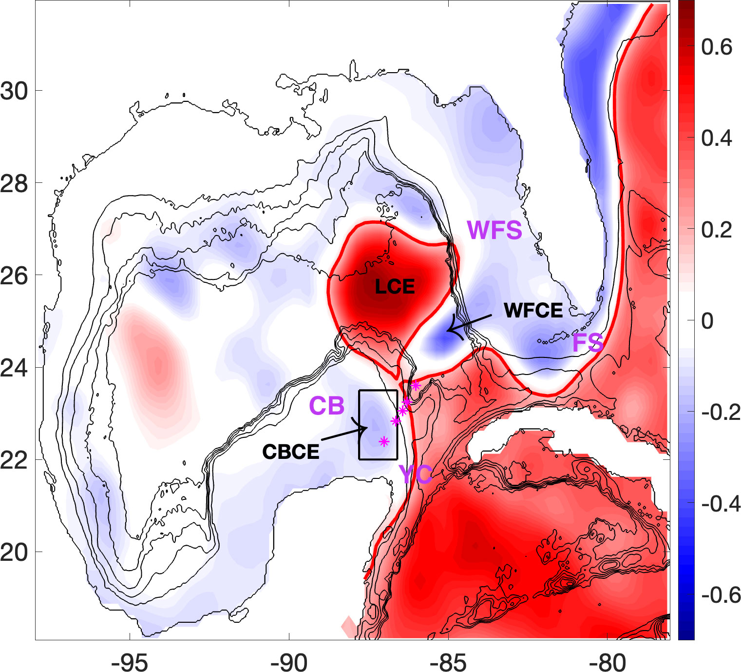
Figure 1 Altimetry sea surface height (SSH, m) during LCE Franklin detachment on 05/29/2010. The red line, which is 0.17 m SSH contour, delineates the edge of the LC. Two LCFEs are present on either side of the LC, the West Florida cyclonic eddy (WFCE) on the east flank of the LC and the Campeche Bank cyclonic eddy (CBCE) the west flank of the LC. The mooring stations described in Section 2.3 are marked in magenta asterisks. Acronyms of geographic features are in magenta text: West Florida Shelf (WFS), Florida Straits (FS), Yucatan Channel (YC) and Campeche Bank (CB). The rectangular region that contains the CBCE is the fixed region in which the spatially averaged potential vorticity of eastern CB is estimated in Section 3.1 and 3.2. The black lines are isobaths from 0 to 3000 m with 600 m intervals.

The layout of this article is as follows: Section 2 provides background information about the ensemble simulation and a description of the observational data. Section 3 presents the research results, including the impact of initial conditions on the LC system, the teleconnection found between LCFEs and a model-mooring data comparison. Section 4 provides a summary and a discussion.

2 Background/model description

2.1 HYCOM setup

The ensemble forecast we used was generated using the Hybrid Coordinate Ocean Model (HYCOM) (Bleck, 2002; Chassignet et al., 2003; Halliwell, 2004). The model configuration is described in Iskandarani et al. (2016). HYCOM uses a generalized vertical coordinate system to optimize the distribution of vertical computational layers so that they are isopycnic (sigma) in stratified regions, terrain-following in shallow coastal regions, and isobaric (z-level) in the unstratified mixed layer. The model used here has a horizontal grid resolution of 1/25° and 20 vertical layers². Out of the vertical layers, 5 are purely z-levels at the top, and spread to about 20 m depth in the open ocean, ensuring a good representation of the upper ocean, while the other 15 layers are hybrid (z-levels, sigma or terrain-following depending on the stratification and on the location) to represent the rest of the water column. The computational domain is open along portions of its southern, eastern and northern boundaries, where values are provided by a lower resolution 1/12° North Atlantic HYCOM simulation (Chassignet et al., 2007). The model is forced by the 27km resolution Coupled Ocean Atmosphere Mesoscale Prediction System (COAMPS) atmospheric outputs ³. The model has the same configuration as the GoM regional expt 20.1 experiment of HYCOM (McDonald, 2006) that was implemented in near realtime by the US Navy Research Laboratory (NRL) at the time of Eddy Franklin, which ensures that it is a robust model with realistic capabilities. In particular, the expt 20.1 experiment was used in several studies of the Deepwater Horizon oil spill (e.g. Mezić et al. (2010); Liu et al. (2011); Valentine et al. (2012); Le Hénaff et al. (2012b)). The initial conditions for the model, prior to perturbations, are from the same expt 20.1 experiment which assimilates available satellite altimeter observations and in situ sea surface temperature (SST) as well as available in situ vertical temperature and salinity profiles from XBTs, ARGO floats and moored buoys. After adding perturbations, the model is then integrated forward in time without data assimilation.

2.2 The HYCOM Ensemble

Each member (or realization) of the ensemble, which is integrated for 60 days from May 1, 2010 to June 29, 2010, corresponds to a different initial condition in which the size and strength of the West Florida Cyclonic Eddy (WFCE) are modified with respect to the control run, which is the unperturbed simulation. The perturbation strategy is based on the Empirical Orthogonal Function (EOF) decomposition of the temporal evolution of the near-real time, data-assimilative expt20.1 experiment from which the present model configuration is derived. The EOF decomposition was computed over a 14-day period, which is expected to be dominated by changes in the LC and LCFEs (Iskandarani et al., 2016). The multivariate, 3-dimensional EOF decomposition is performed on two variables: the 3-dimensional ocean hydrostatic pressure increment in each model layer, and the sea surface height (SSH). The hydrostatic pressure increment is a good proxy for the ocean vertical structure, in particular the density gradients are associated with geostrophic currents, whereas the SSH incorporates the surface signature of the dynamical features of interest here, i.e. the LC and the associated eddies. The principal components of each mode were used to project the EOF modes to the model prognostic variables, i.e., temperature, salinity, velocities, layer thicknesses (Li et al., 2016). The perturbations consist in the first two leading EOF modes, and the strength of the perturbations to the HYCOM control was modulated by the amplitudes of the EOF modes which were considered uncertain. Iskandarani et al. (2016) shows that the two leading EOF modes mostly perturb the strength of the WFCE. This approach allows us to directly link the output of the simulation to only two uncertain parameters, as done by Iskandarani et al. (2016) and Wang et al. (2018), and provide the opportunity to investigate the relationship between the initial strength and size of the WFCE and the subsequent LC detachment and formation of the Campeche Bank Cyclonic Eddy (CBCE). The first two EOF modes have been found to be sufficient to represent the uncertainty in the Loop Current region from May 1, 2010 to May 30, 2010, when the first detachment of Eddy Franklin occurred (Iskandarani et al., 2016; Wang et al., 2018). Each ensemble member corresponds to a specified setting of the EOF modal amplitudes, referred to here as ξ₁ and ξ₂ (a value of 0 corresponds to not perturbing the control run whereas a value of ±1 corresponds to adding and subtracting the EOF mode at full amplitude). Illustrations of the signature of these perturbations can be found in Iskandarani et al. (2016) (their Figures 1, 2 and 4) and Wang et al. (2018) (their Figure 8). The ensemble sampled the 2D uncertain amplitude space (ξ₁,ξ₂) ⁴ using a total of 49 realizations. The ensemble outputs are saved daily for 60 days from May 1st, 2010 to June 29, 2010. Previous studies showed that the actual LC contour derived from satellite observation generally fall within the envelope of this HYCOM ensemble contours within 30 days, which stresses the realism of the ensemble since the observational data appears to be a plausible realization of the model ensemble (Iskandarani et al., 2016; Wang et al., 2018).

2.3 Mooring data

The observation data used in our study is from the moorings of the Centro de Investigación Científica y de Educación Superior de Ensenada (CICESE) array in the Mexican waters of the GoM. The array was designed to investigate the flow over the Western Yucatan Channel and Campeche Bank and its role in the LC dynamics and LCE detachments (Sheinbaum et al., 2016). The Plataforma Este (PE, Eastern shelf) mooring section that we picked for the analysis crosses from the CB shelf break to depths between 2000 and 3500 m. Section PE is located in the region where CBCEs usually develop. The section consists of five moorings that use a variety of current measurement equipment, such as Acoustic Doppler Current Profilers and Nortek Aquadopp current meters. The moorings are off-shore from 100 km to 270 km. The coordinates of each PE mooring station are listed on Table 2 in Athie et al. (2014). The mooring measurement depth is 100 m for the shallowest station, and it reaches about 3500 m depth for the deepest station. The vertical sampling deployment is at intervals of 300 m to 500 m. The PE section deployment covers over 22 months, from June 2009 to April 2011 (Athie et al., 2014).

3 Results

3.1 Potential vorticity anomaly analysis

Firstly, we investigate the impact of initial condition perturbations on the evolution of the LCFEs’ structure and strength, using potential vorticity (PV) and PV anomaly (PVA) for the dynamical analysis. In geostrophic balance, an eddy is associated with a local extreme of PV (Ertel, 1942). In isopycnal coordinates, the PV of a fluid parcel within an isopycnal layer is given by

where ζ is the relative vorticity of the fluid within the layer, h is the layer thickness, and f is the planetary vorticity. The PV includes information of both the vorticity dynamics (numerator) and the mass field (denominator). PVA is defined as the difference between PV and a reference PV state at rest (PVref), which was chosen here to be the ocean at a location outside the LC and LCFE regions (calculation details of PVref provided later on), normalized by the reference layer thickness H

Hoskins et al. (1985) found that the presence of a PVA pole in a specific layer is associated with a circulation that extends to all layers, but which is more intense in that specific layer (a positive PVA pole being associated with a cyclonic circulation, while a negative PVA pole is associated with an anticyclonic circulation). That property means that the strengthening of the cyclonic structure, can be associated with an intensification of its PVA [see also Herbette et al. (2005); Meunier et al. (2010); Le Hénaff et al. (2012a)]. Thus, the PVA evolution of the LCFEs reveals the strengthening or weakening of the LCFEs’ structures.

There are 20 hybrid layers in the original HYCOM output. To simplify the analysis, we group together those original layers with similar PVA patterns and come up with a simplified two-layer system. Previous studies have conducted similar layer simplification strategy to analyze the evolution of LCFE (Le Hénaff et al., 2012a; Androulidakis et al., 2014). To get the simplified system, we first project the model outputs onto purely isopycnal layers, using the same number of layers, as well as the same target densities as the native HYCOM grid. The projection on purely isopycnal layers is necessary, because the PV calculation requires the knowledge of isopycnal layer thicknesses. This projection procedure leads to the interpolation of fields only from the layers that were not isopycnal in the HYCOM configuration, i.e., layers that were based on z levels and sigma layers near steep topography. The new fields in the purely isopycnal layers are interpolated linearly between adjacent depths from the original HYCOM grid. To define PV_ref in our study, we select a date in the previous year in the same season when the LC is not as extended. On that date, we select a grid point in the eastern Gulf which is away from both the LC and LCFE regions, to estimate the reference PV, using outputs from the near-real time HYCOM expt_20.1 reference experiment. The LC dynamics is absent from the location selected for estimating PVref location, and RV at the reference location is as close to zero as possible, so that the ocean state used to estimate PVref can be considered at rest when compared to the LC system. The same approach was used by Le Hénaff et al. (2012a) and Androulidakis et al. (2014) to study the evolution of the LCFEs and of the LC system. PVref in each isopycnal layer is calculated as $P{V}_{\text{ref},i}=\frac{f}{H_i}$, where PV_ref,iis the reference PV corresponding to the i-th isopycnal layer, and H_iis the i-th HYCOM layer depth at the reference point.

After projecting the original hybrid HYCOM layers into purely isopycnal layers and after defining PV_ref, we estimate the PVA in each layer in order to identify the positive PVA regions along the west Florida Shelf and over the Campeche Bank corresponding to the cyclonic activities associated with the west Florida cyclonic eddy (WFCE) and the Campeche Bank cyclonic eddy (CBCE), respectively. After identifying the layers showing the high positive PVA signals associated with the cyclones under study, we reduce the number of layers in order to simplify the analysis of the evolution of the PV field. The isopycnal layers with a high positive PVA cores corresponding to WFCE and CBCE are grouped together. In our case, this method leads to a simplified analysis using two layers, where the LC and LCFEs signals are mainly in the upper layer. The upper layer groups the top 10 projected isopycnal layers of densities ranging from 1019.5 to 1025.77 kg/m³ and extends as deep as 800 m in the study area, while the lower layer below extends to the GoM bottom. We then evaluate the corresponding PVA for each simplified layer. We use vertically averaged velocity for the calculation of relative vorticity ζ, and the layer thickness h is the sum of the thicknesses of all the isopycnal layers that constitute the simplified layer.

We focus on the evolution of LCFEs in several specific ensemble members with significantly different initial condition perturbations: realization 01(hereafter RZ01) with the most negative perturbations [(ξ₁,ξ₂) = (−0.9491,−0.9491)], realization 25 (hereafter RZ25) with no perturbation [(ξ₁,ξ₂) = (0,0)], a.k.a., the control run, and realization 49 (hereafter RZ49) with the most positive perturbations [(ξ₁,ξ₂) = (0.9491,0.9491)]. Figure 2 shows the upper layer PVA evolution of our simplified two-layer system for those three different realizations. The differences in PVA anomaly on the first day are due to the initial condition perturbations. RZ49 has the most positive PVA and the largest high positive PVA region to the north and northeast of the extended LC, while RZ01 has the least positive PVA and smallest high positive PVA region. The control run RZ25 has a moderate positive PVA strength and positive PVA size region. This illustrates how the initial condition perturbations perturb the strength of the WFCE, and also the northern cyclonic eddy (NCE) (Schmitz, 2005), which is located on the northern edge of the LC. A positive perturbation yields strong frontal eddies and vise versa. This relationship between perturbation and the strength of the LCFEs matches the results from Iskandarani et al. (2016), who found the same effect of the initial condition perturbations on the strength of the WFCE, albeit in the SSH signal. As time progresses, the positive PVA pattern corresponding to the WFCE moves southward along the west Florida shelf before it changes direction to intrude into the LC. On day 20, the three realizations differ in the degree to which the WFCE has intruded into the LC. RZ49 shows a WFCE with the most western longitudinal extension and whose PVA remains the most intense among the three realizations. When the perturbation is negative, in RZ01, the western intrusion of the WFCE into the LC is reduced along with its amplitude. On day 30, the WFCE in RZ01 moves south along the shelf, instead of intruding west into the LC, while its counterparts in RZ25 and RZ49 continue their westward intrusion. The WFCE in RZ49 still exhibits a stronger positive PVA than that in RZ25, and more importantly, the former has evolved into an extended tongue that intrudes further west than 88°W, which makes the LCE totally detached. Based on the 17-cm SSH contours (not shown) that Leben (2005) used to define the edge of the LC, on day 30 RZ49 has a detached LCE, RZ25 shows a nearly detached LCE, and RZ01 has no tendency of LCE detachment at all. It is also worth noticing the PVA evolution on the eastern edge of the CB. From day 1 to day 20, high PVA accumulates gradually over the eastern CB close to the Yucatan, as the LC is squeezed against the CB. The PVA evolution in this region is similar across the realizations during this period. On day 30, the three realizations show evident differences in PVA patterns over the eastern CB. In RZ25, the high positive PVA region along the eastern bank edge is more intense than that in RZ01, and in both realizations, it is oriented along the southeast-northwest direction, following the edge of the LC. In RZ49, this area of high PVA starts to move northeastward and to interact with the southwestward moving WFCE; this growing patch of high positive PVA eventually forms a CBCE. To sum up, Figure 2 delivers the information that PV along the CB accumulates and finally forms a CBCE when the WFCE is strong and intrudes into the LC, while no CBCE forms when the WFCE is initially weak and LC intrusion does not happen. In Subsection 3.2, we perform an analysis of the teleconnection taking place between the WFCE and the CBCE.

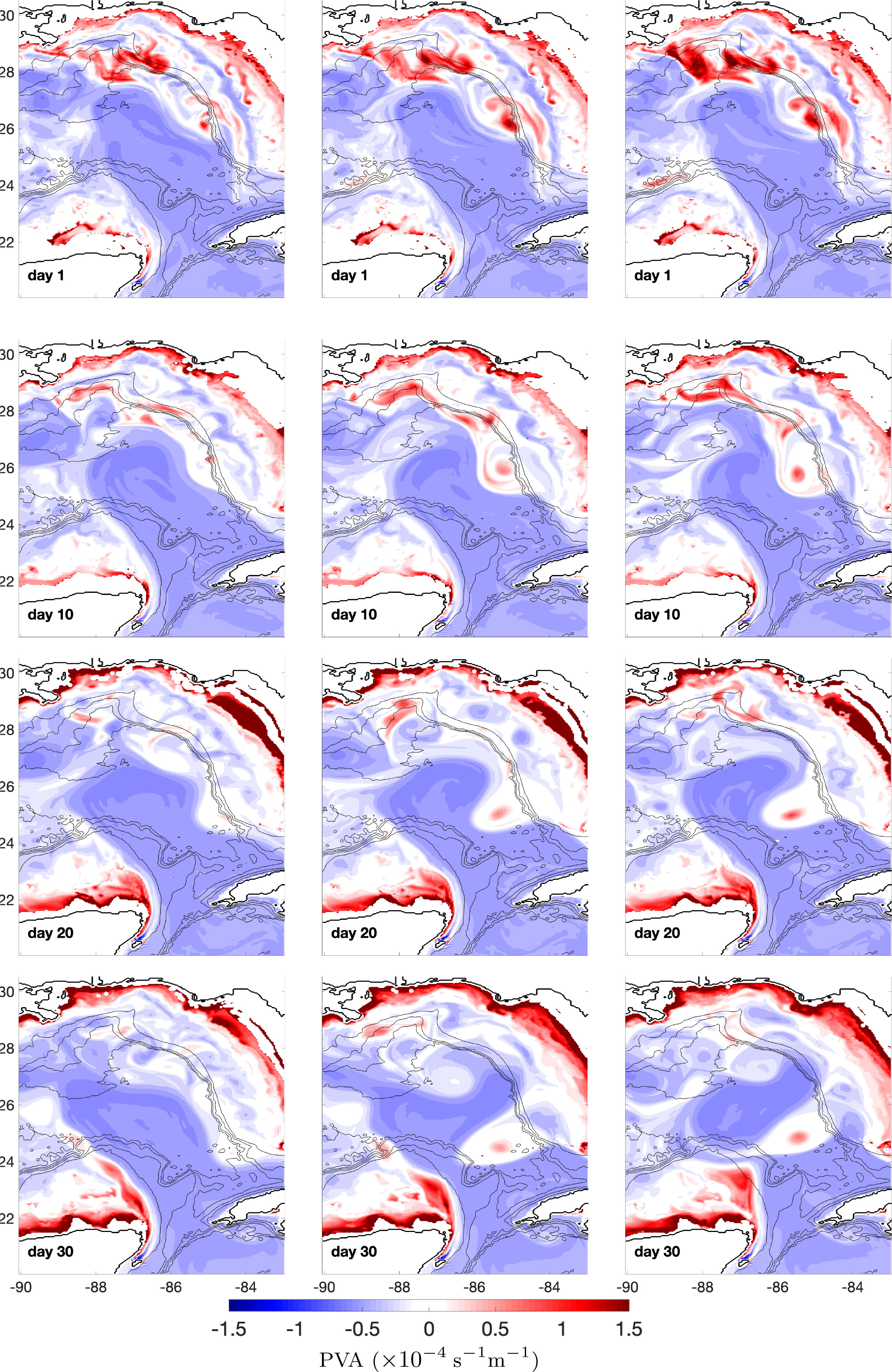
Figure 2 Upper layer PVA evolution for RZ01 (left column), RZ25 (center column), and RZ49 (right column). Coastlines are shown in black lines. Isobaths are shown in gray lines from 0 to 3500 m with 700 m intervals.

Figure 3 shows the evolution of the lower layer PVA for the three realizations. Realizations showing a strong WFCE signals in the upper layer (see RZ25 on day 20 and 30, and RZ49 for day 10, 20 and 30) have corresponding strong pole in positive PVA in the lower layer. This indicates that the WFCE, once well developed, has a very coherent vertical structure, which is consistent with Le Hénaff et al. (2012a). All three realizations show a strong positive PVA belt along the eastern edge of the CB from day 1 to day 20. This belt stretches from the eastern shelf along the Yucatan Peninsula in the Caribbean Sea (20° N) to the northern tip of the CB (24°N).

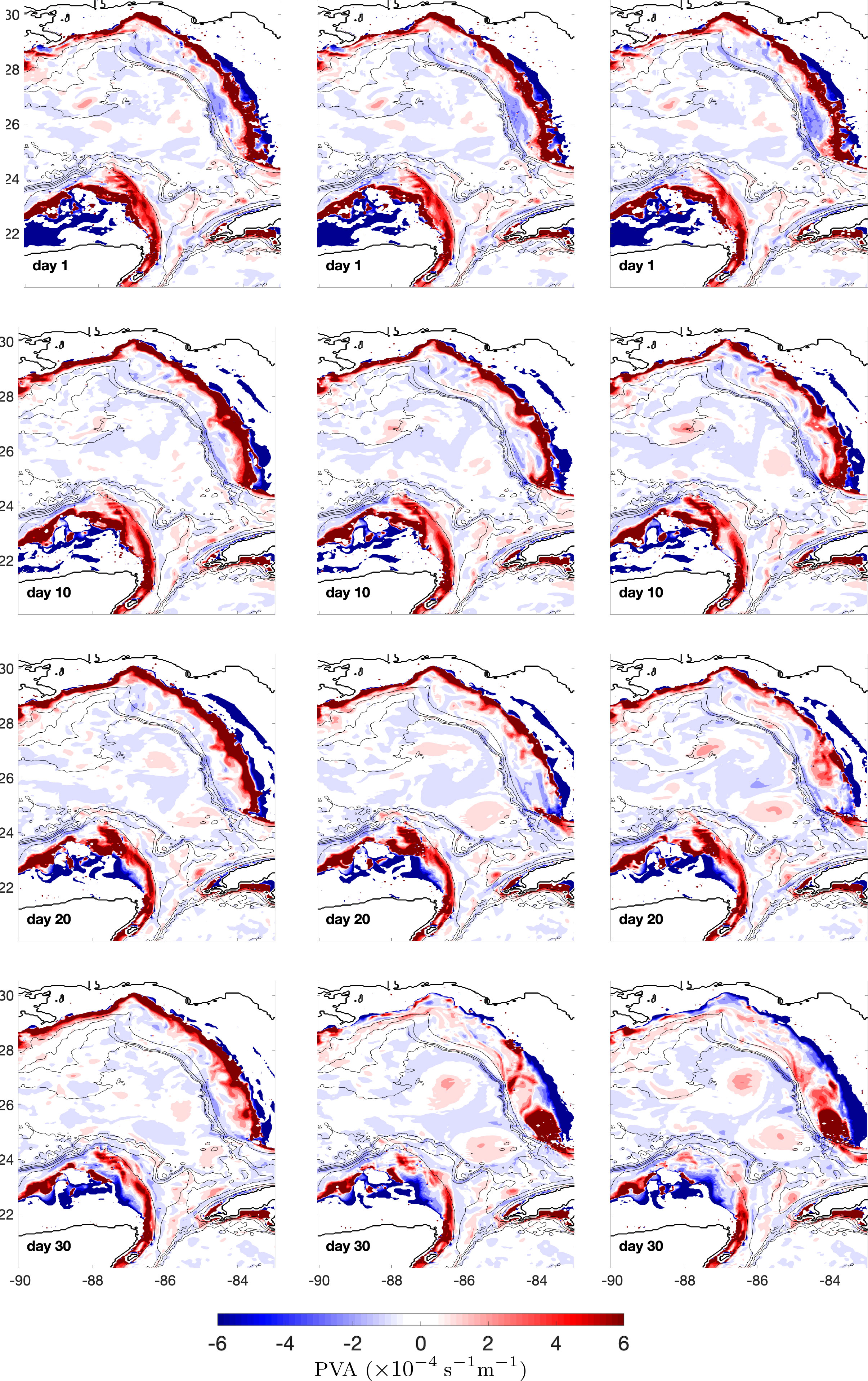
Figure 3 same as Figure 2, for lower layer PVA evolution.

In RZ49, where CBCE is in development in the upper layer, this strong positive belt in the lower layer retracts (from 24°N to 23°N) on day 30. This indicates that, when the upper layer high positive PVA patch along the eastern CB starts to shift direction to the northeast, developing a CBCE (RZ49), its lower layer PVA structure erodes. While in the simulations that this upper layer PVA patch is oriented southeast- northwest (RZ01 and RZ25), the PVA belt in the lower layer does not erode.

Figure 4 presents the evolution of the ensemble upper layer PVA standard deviation ⁵ as a measure of the uncertainty in the PVA in the simplified upper layer associated with the variability of the ensemble of initial conditions. In the early stage (from day 5 to day 20), the PVA uncertainty is mainly located to the north and northeast of the LC. The region of high PVA variance east of the LC is due to the different strength and size of the WFCE across realizations. At day 25, a noticeably high PVA variance region starts to form over the eastern CB, and becomes significant on day 30. It reflects that a CBCE has formed in some realizations while fail to form in other realizations. This corresponds to the difference in the CBCE formation and the LCE detachment across the different realizations.

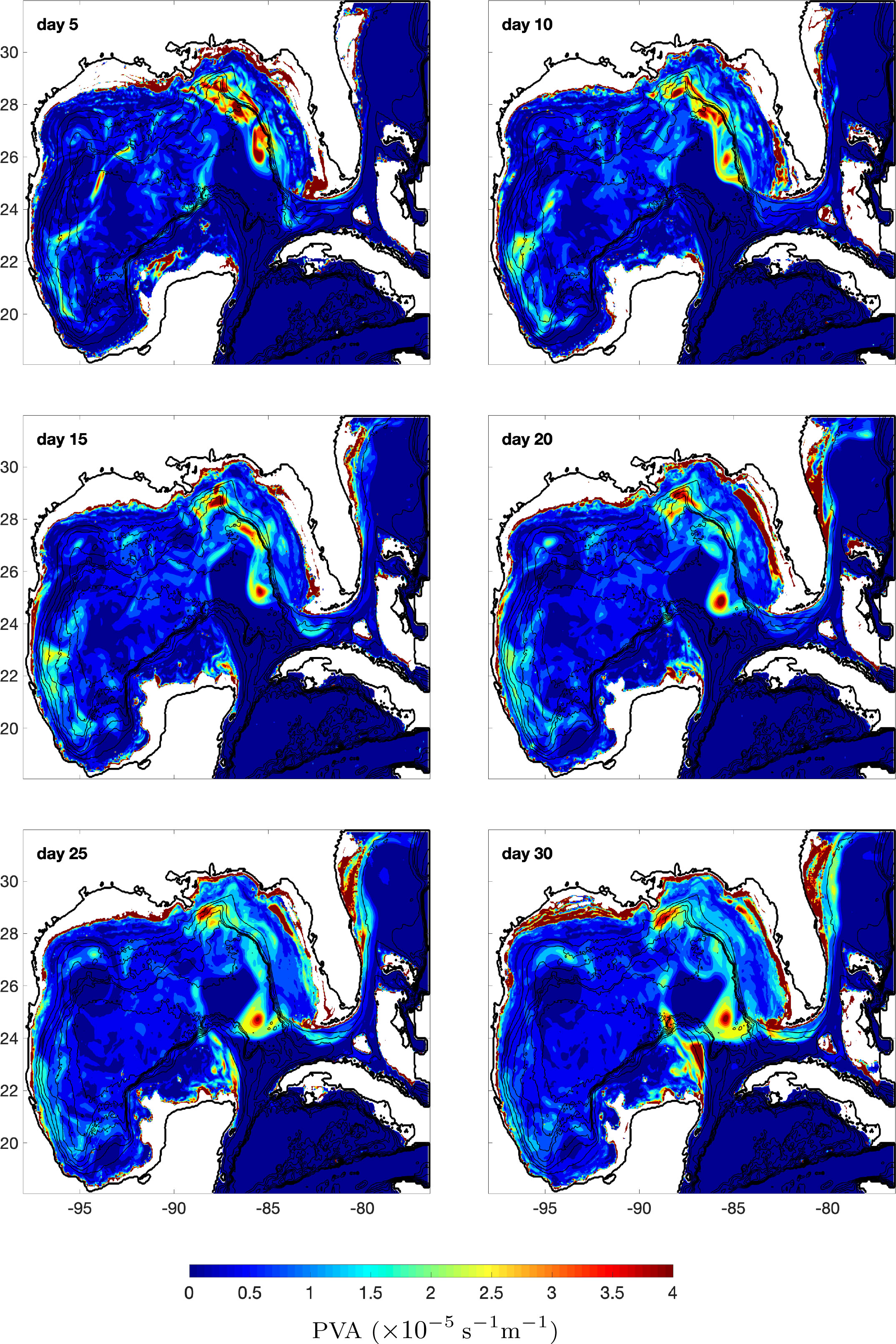
Figure 4 Ensemble standard deviation of PVA in the upper layer. The black lines are isobaths from 0 to 4000 m with 500 m intervals.

We now investigate the relationship between the EOF perturbation stochastic amplitudes, ξ₁ and ξ₂, the initial size and strength of the WFCE, and the later development of CBCE. We use the -28 cm SSH to define the edge of the WFCE region as in Hiron et al. (2020) where this contour level was found to be a good and convenient proxy for attractive Lagrangian Coherent Structures (closed patterns of high negative values of the finite-size Lyapunov exponent). Figure 5 shows the response surfaces of the initial area size and strength (defined as the spatially integrated PV) of the WFCE at day 1 to changes in the stochastic amplitudes ξ₁ and ξ₂. The two quantities show a strong dependence to the amplitude of the first EOF mode ξ₁. With an increase of ξ₁, both the size and strength of WFCE increase evidently. With different values of ξ₁, the initial strength of WFCE can vary from 0.07×10⁻⁴ to 2.98×10⁻⁴ s⁻¹m⁻¹, the initial size of WFCE from 0.23×10³ to 11.6×10³ km². By contrast, the WFCE is quite insensitive to changes in ξ₂. The difference in sensitivity of the WFCE characteristics to the two perturbation modes can be explained by the spatial signature of these EOF modes: mode 1 has a strong signature on the initial WFCE, whereas the signature of mode 2 in the WFCE is not as strong (see Iskandarani et al. (2016), their Figure 1). In addition, the explained variance of EOF mode 2 is quite small compared to that of EOF mode 1 (Iskandarani et al., 2016). As a result, ξ₂, the amplitude of mode 2, has little impact on WFCE, and EOF 1 makes the largest contributions to the perturbation of the initial size and strength of WFCE.

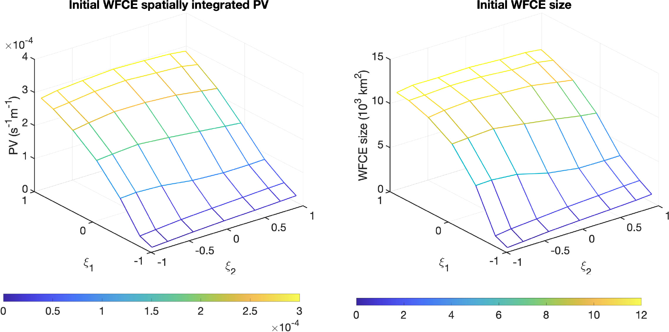
Figure 5 Spatially integrated PV of WFCE (left) and its size (right) on day 1 over the stochastic variable space.

Figure 6 shows the temporal evolution of the response surface of the spatially integrated PV over the eastern CB (see Figure 1), where we found that the PVA variance increases after day 25 (see Figure 4). On day 5, the averaged PV over this region is insensitive to changes in ξ₁ or ξ₂. As time progresses, however, the dependence of the area-integrated PV on ξ₁ starts to appear whereby an increase in ξ₁ leads to an increase of the area-integrated PV. The area-integrated PV remains largely insensitive to changes in the amplitude of the second mode ξ₂ throughout the duration of the experiment albeit for slight positive correlation. Although the change of the area-integrated PV along the ξ₁ axis is not monotonic in some realizations, it is obvious that the increase in PV over the CB since day 25 is strongly associated with increasing ξ₁, that is an increase in the size and strength of the WFCE. The area-integrated PV of all realizations increases with time, with the largest increase associated with those realizations with a strong and large initial WFCE (high ξ₁). Figure 6 confirms that, although the initial impact of the the 1st EOF mode perturbation is confined to the northeast of the LC, it leads to a stronger subsequent PV development southwest of the LC along the eastern CB.

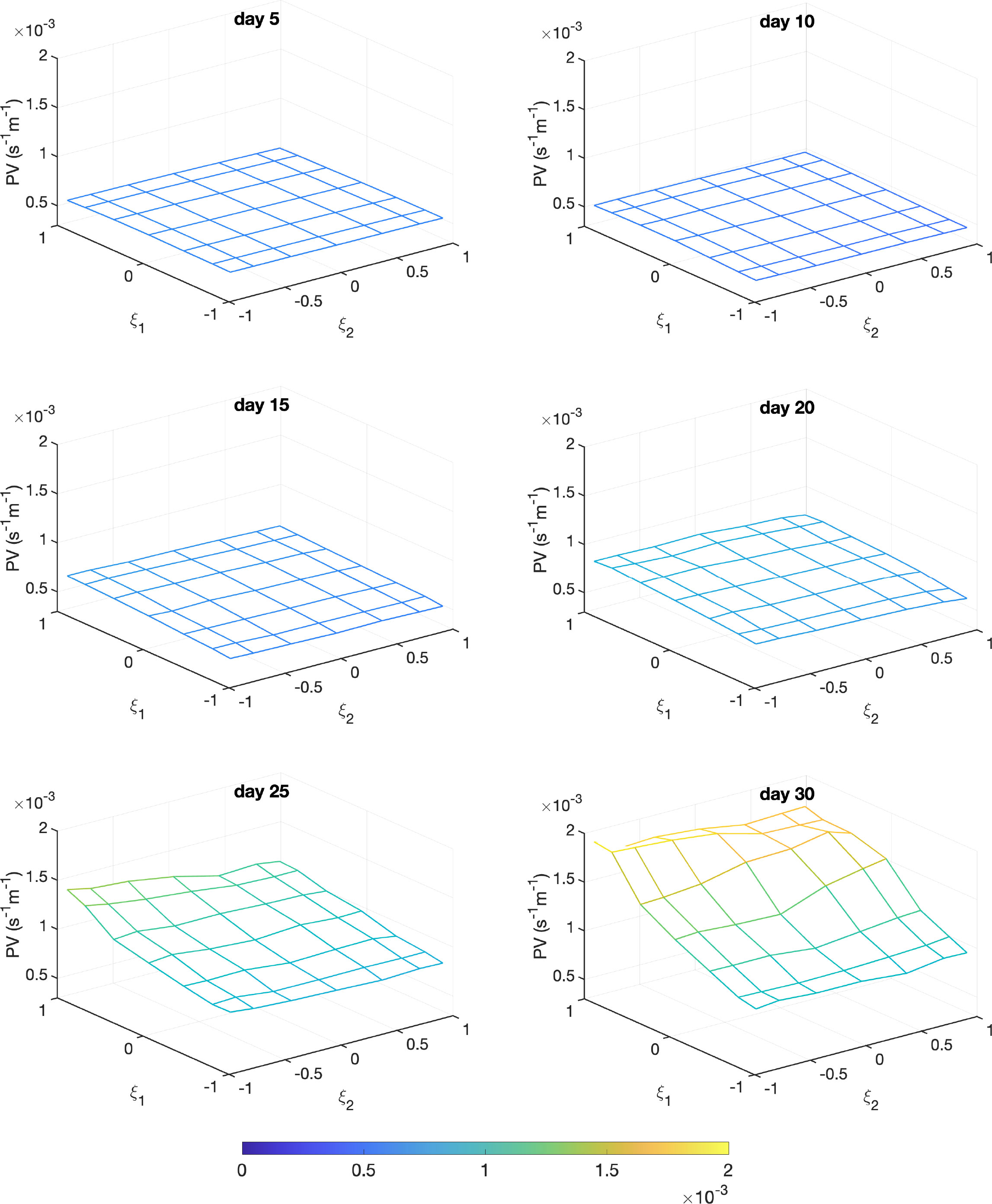
Figure 6 Evolution of spatially integrated PV over the eastern CB in the stochastic variable (ξ₁, ξ₂) space.

3.2 Teleconnection between LCFEs

The initial condition perturbations modify the PVA in the northeastern GoM and modulates the strength of the WFCE. These same perturbations do not impact the PVA over the eastern CB until 25 days later when differences between realizations starts to appear appear, especially along the CB. In order to investigate whether the PV evolution over the eastern CB can be correlated with other processes in the GoM, we estimate the covariance between the spatially averaged upper layer PV over the eastern CB on day 30 (22.4° N to 23.8° N, 86.6° W to 87.8° W, see the rectangular region in Figure 1) and the SSH with lagged time over the whole GoM.

For two variables X and Y, the covariance is estimated as

For covariance between the spatially averaged PV over eastern CB on day t, $P{V}_{CB}^t$, and the SSH at a grid (i,j) with τ days lag, $SS{H}_{ij}^{t-\tau }$, the empirical covariance between them is

Where $P{V}_{CB,n}^t$ is the spatially averaged PV of CBCE on day t for realization number n, $SS{H}_{ijn}^{t-\tau }$ is SSH value at grid point (i,j) with τ days lag for realization number n,$\overline{P{V}_{CB}^t}=\frac{1}{N}{\displaystyle \sum _{r=1}^N}P{V}_{CB,n}^t,\overline{SS{H}_{ij}^{t-r}}=\frac{1}{N}{\displaystyle \sum _{r=1}^{N}SS{H}_{ijn}^{t-r}}$, N is the total number of realizations.

Figure 7 shows the covariance between this averaged PV on day 30, and the lagged SSH (SSH on day 5, 10, 15, 20, 25 and 30) over the entire GoM. The covariance is normalized by the maximum and minimum values so that all the values fall between -1 and 1. On day 5, i.e., at -25 day lag, negative covariance regions is present on the northeast side of the LC and these regions overlap with the front of the WFCE shown in SSH contours. As time progresses, this negative covariance strengthens and the associated region moves along with the WFCE front. The ensemble mean SSH contours are shown as well, in black lines. On day 25, i.e., at -5 day lag, on the north and east side of this negative covariance region, noticeable positive covariance emerges, which coincide with the LC edges that have been displaced westward by an intruding WFCE. On day 30, i.e., at 0 day lag, the negative covariance region extends to the east side of the CB, while the positive covariance regions intensify. Since a cyclonic eddy is associated with a negative SSH anomaly and an anti-cyclonic is associated with a positive SSH anomaly, a negative covariance with the SSH of a cyclonic eddy corresponds to a positive relationship with the strength of that eddy. This covariance analysis stresses the statistical teleconnection that exists between the signatures of both LCFES at various times, i.e., the CBCE around the time of its formation and the WFCE during the previous 25 days.

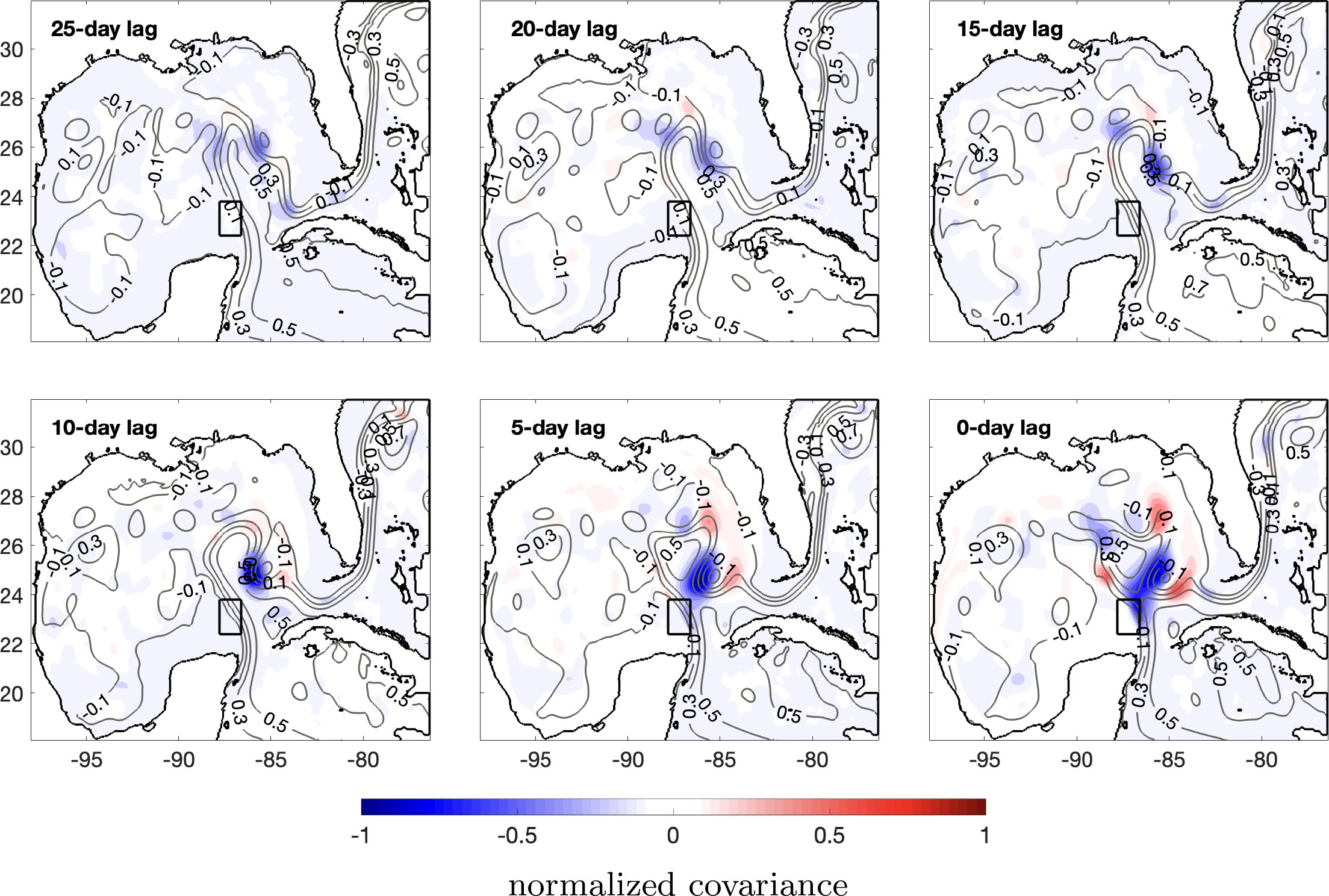
Figure 7 Covariance between the spatially averaged upper layer PV over the eastern CB on day 30 (the spatially averaged area shown in rectangular region in each subplot, and in Figure 1 as well) and the lagged SSH (SSH on day 5, 10, 15, 20,25 and 30) over the GoM. The covariance is normalized by the maximum and minimum values so that all the values fall between -1 and 1. The ensemble mean SSH contours are shown in gray lines marked with SSH values (in m). The coastlines are shown in black lines.

Figure 8 is the scatterplot of initial WFCE strength versus area-integrated PV over the eastern CB. The red circles are realizations without an LCE detachment occurs and the blue circles are realizations where an LCE detachment occurs. The correlation coefficient r between both variables is already high on day 1, and reaches its peak value of 0.945 on day 30. The correlation weakens slightly on day 35 but still exhibits a high correlation coefficient. Figure 9 is the scatterplot of the initial WFCE size versus the eastern CB strength. The result is quite similar to that of Figure 8. The correlation between the initial WFCE size and the eastern CB strength remains high throughout all the forecast days and it peaks on day 30. The positive correlation between the initial WFCE size and the integrated PV over the eastern CB, illustrative of a teleconnection between both eddies, is verified in Figures 8, 9. Another phenomenon that is revealed in Figures 8, 9 is that the realizations with an LCE detachment start with an initially higher WFCE strength and size, and end with a higher eastern CB integrated PV value, than those without LCE detachment. In the realizations without an LCE detachment, the initial integrated PV values of WFCE are all lower than 1.5×10⁻⁴s⁻¹m⁻¹. Most of the PV values are greater than 1.5×10⁻⁴s⁻¹m⁻¹ for realizations with an LCE detachment, except for three realizations, whose PV values are around 0.8×10⁻⁴s⁻¹m⁻¹. Similarly, in terms of the initial WFCE size, the realizations without an LCE detachment have small WFCE sizes that are always smaller than 6×10³km². The initial WFCE size is greater than 6×10³km² for the realizations with an LCE detachment, with 3 exceptions, which are all around 4×10³km². In terms of the eastern CB integrated PV value (y axis values in Figures 8, 9), all the realizations with an LCE detachment have PV values greater than 4.0 ×10⁻⁴s⁻¹m⁻¹ on day 35, while all the realizations without an LCE detachment have PV values lower than 4.0 ×10⁻⁴s⁻¹m⁻¹. By contrast, on day 1, the eastern CB integrated PV values are similar across all realizations.

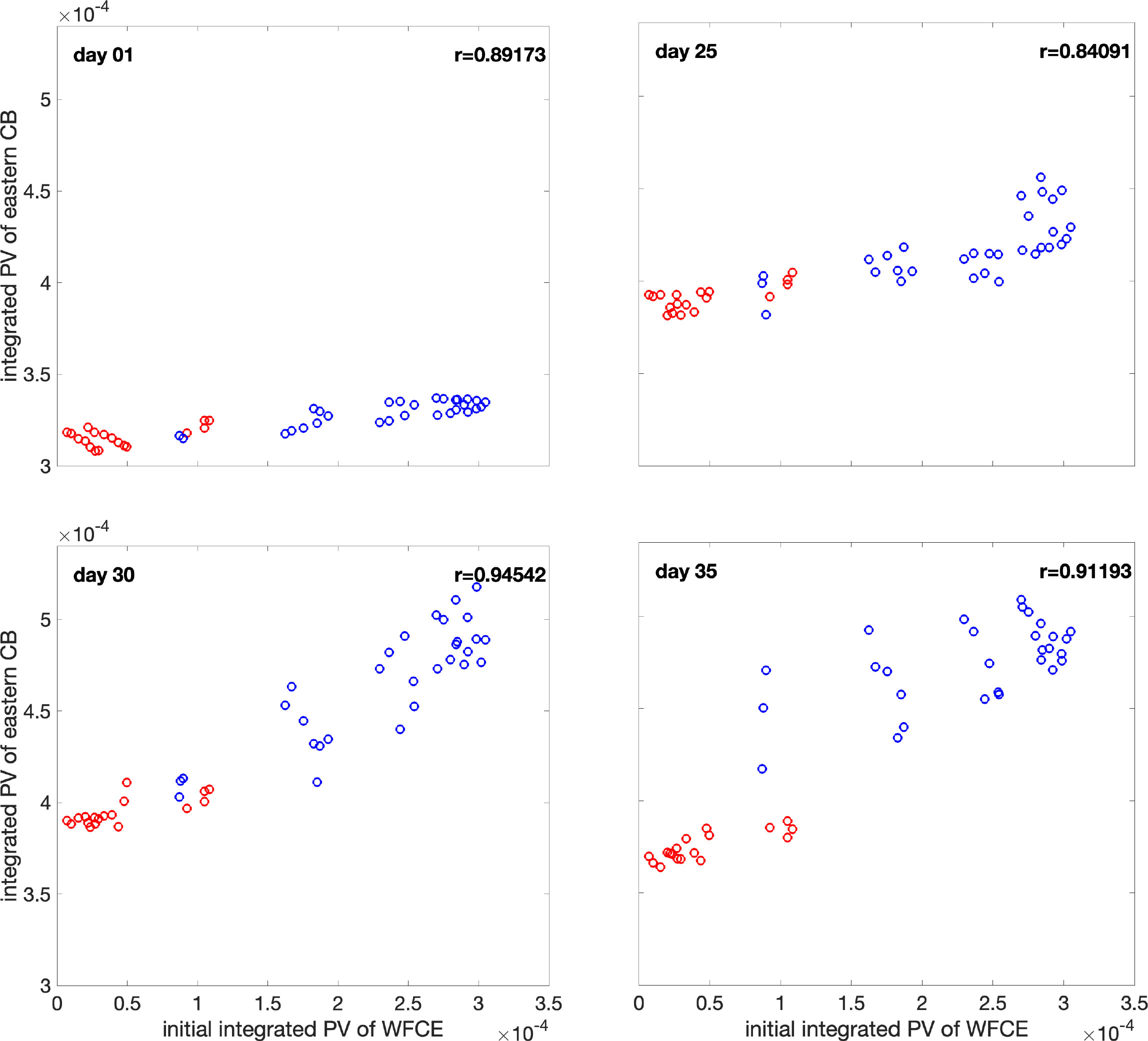
Figure 8 Scatterplots of integrated PV (s⁻¹m⁻¹) over the eastern CB (see box on Figure 1) on day 01, 25, 30 and 35 against the initial day 01 integrated PV of the WFCE. Red circles are realizations without an LCE detachment. Blue circles are realizations with an LCE detachment.

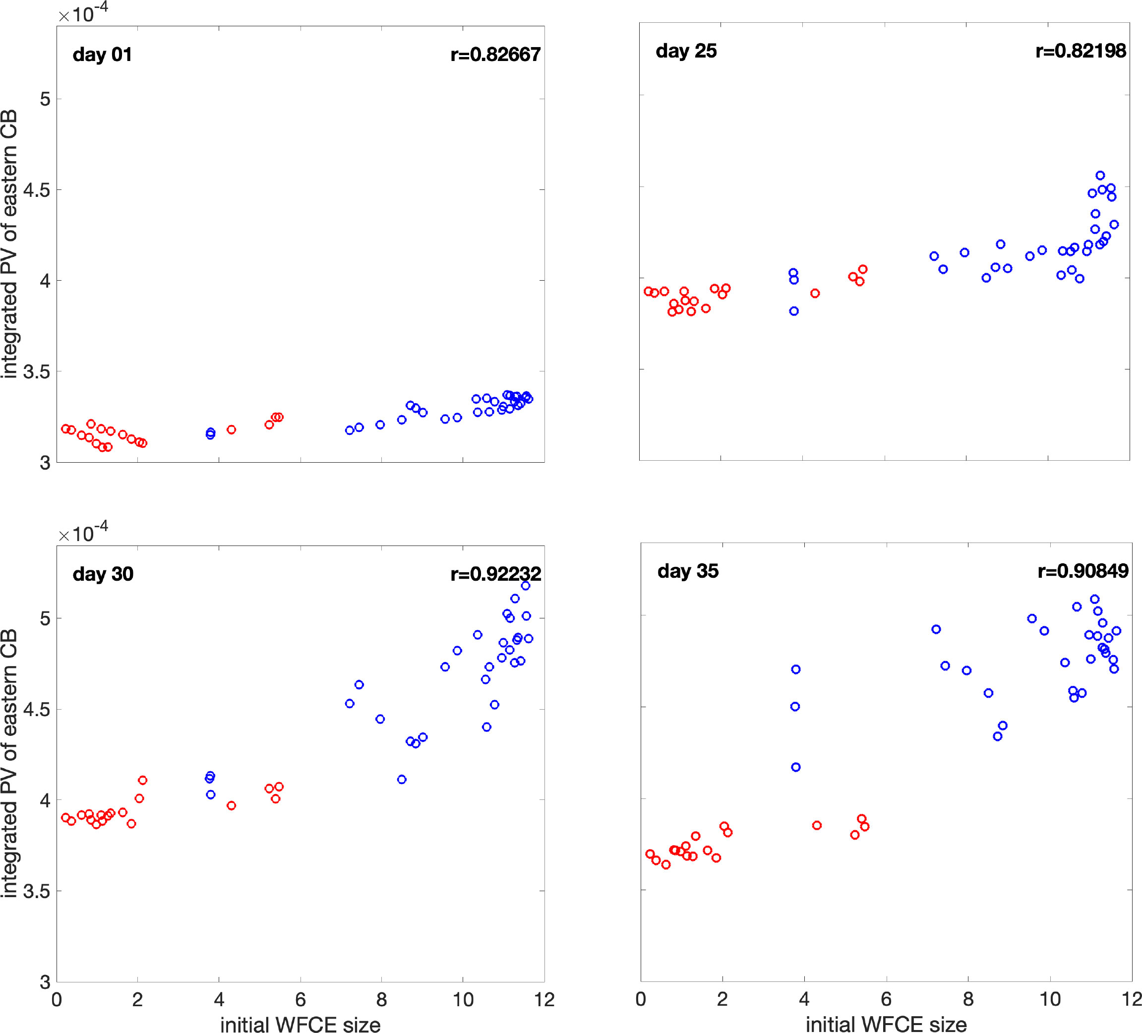
Figure 9 Scatterplots of integrated PV (s⁻¹m⁻¹) over the eastern CB (see box on Figure 1) on day 01, 25, 30 and 35 against initial size (10³km²) of the WFCE. Red dots are realizations without an LCE detachment. Blue dots are realizations with an LCE detachment.

In Subsection 3.1, we showed that a CBCE develops only when a WFCE is strong enough to intrude into the LC. The statistical analysis performed in this subsection confirms that a teleconnection exists between both eddies, during the LCE detachment process, by which the growing PV on the eastern CB is positively related with the strength of WFCE and the distance between them. In other words, a more intense WFCE approaching the CB will lead to increase in the PV over the eastern CB and favor the formation of a CBCE.

3.3 LCE detachment criterion

This subsection presents the investigation of the conditions and timing of the LCE detachment. Among the 49 ensemble realizations, 29 realizations led to an LCE detachment; no such detachment occurs for the remaining 20 realizations in the 60-day simulation period. Figure 10 shows the relationship between the LCE detachment day and the amplitude of the first perturbation ξ₁, since there is little dependency on ξ₂. We can see that in the scatterplot, there is a noticeable negative trend between these two variables. The more positive ξ₁ value, the sooner the LCE detachment. In other words, a larger ξ₁ accelerates the LCE detachment process. The PVA plots on Figures 2, 3 also suggest that the positive initial perturbation is associated with a more unstable LC system, i.e. with large meanders and strong PVA poles. This finding shows that the initial conditions, in particular the strength of the WFCE, have a role on the behavior of the LC system, i.e., the LCE detachment occurrence and timing. This may be useful for LC system forecasting.

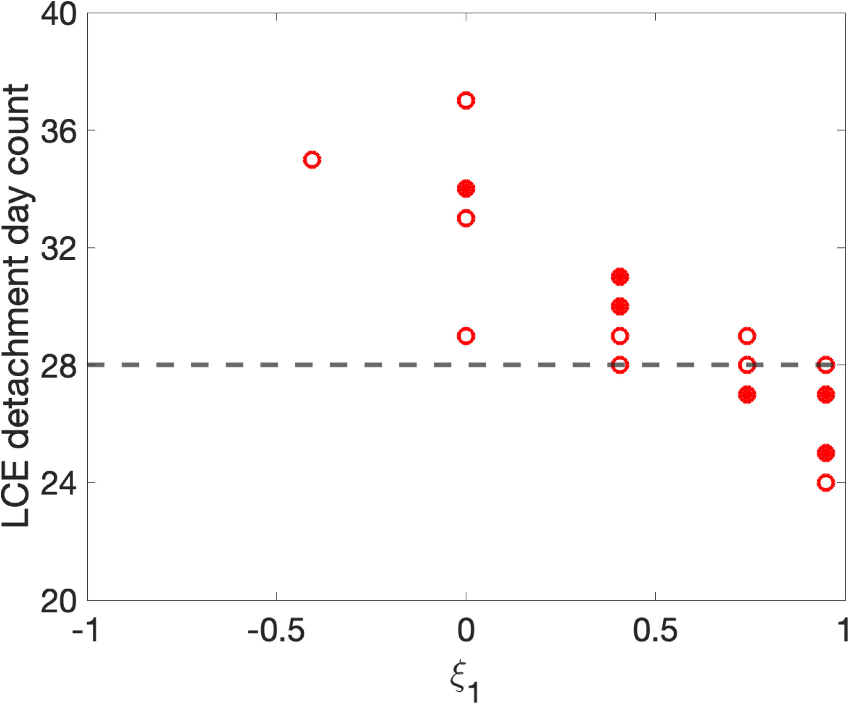
Figure 10 LCE detachment day against ξ₁. Circles are single realizations. Solid dots are multiple realizations that are overlapped. The horizontal dashed line (day 28) is the day that the LCE actually detached based on altimetry data.

We also trace the trajectory of WFCEs in all the ensemble realizations. We find that when an LCE detaches, the western extension of WFCE is always west of 85.6° W (not shown). In the realizations without an LCE detachment, the WFCE is always east of 85.6° W (when the WFCE moves south to 26° N). This is in agreement with mechanisms described by Schmitz (2005), and it reveals that in order to trigger an LCE detachment, the WFCE needs to extend at least west to 85.6°W.

We also present the LCE detachment in altimetry SSH data, to verify that the eddy detachment process that we found in the ensemble of simulations is realistic. Figure 11 shows the altimetry SSH evolution for Eddy Franklin in 2010 (upper row) and Eddy Icarus 2011 (lower row). These two eddy detachment events exhibit WFCEs with similar sizes before the WFCEs start to intrude into the LC. These two events also share a similar LCE detachment mechanism, with the WFCE making the major contribution to the initial eddy detachment. The timespans from the WFCE intrusion to the LCE detachment are similar as well, in these two events, with 26 days for Franklin, and 21 days for Icarus. More generally, the involvement of a strong WFCE and of a growing CBCE, as is the focus of our study, is consistent with Schmitz (2005), who studied and described a large number of LCE detachment sequences.

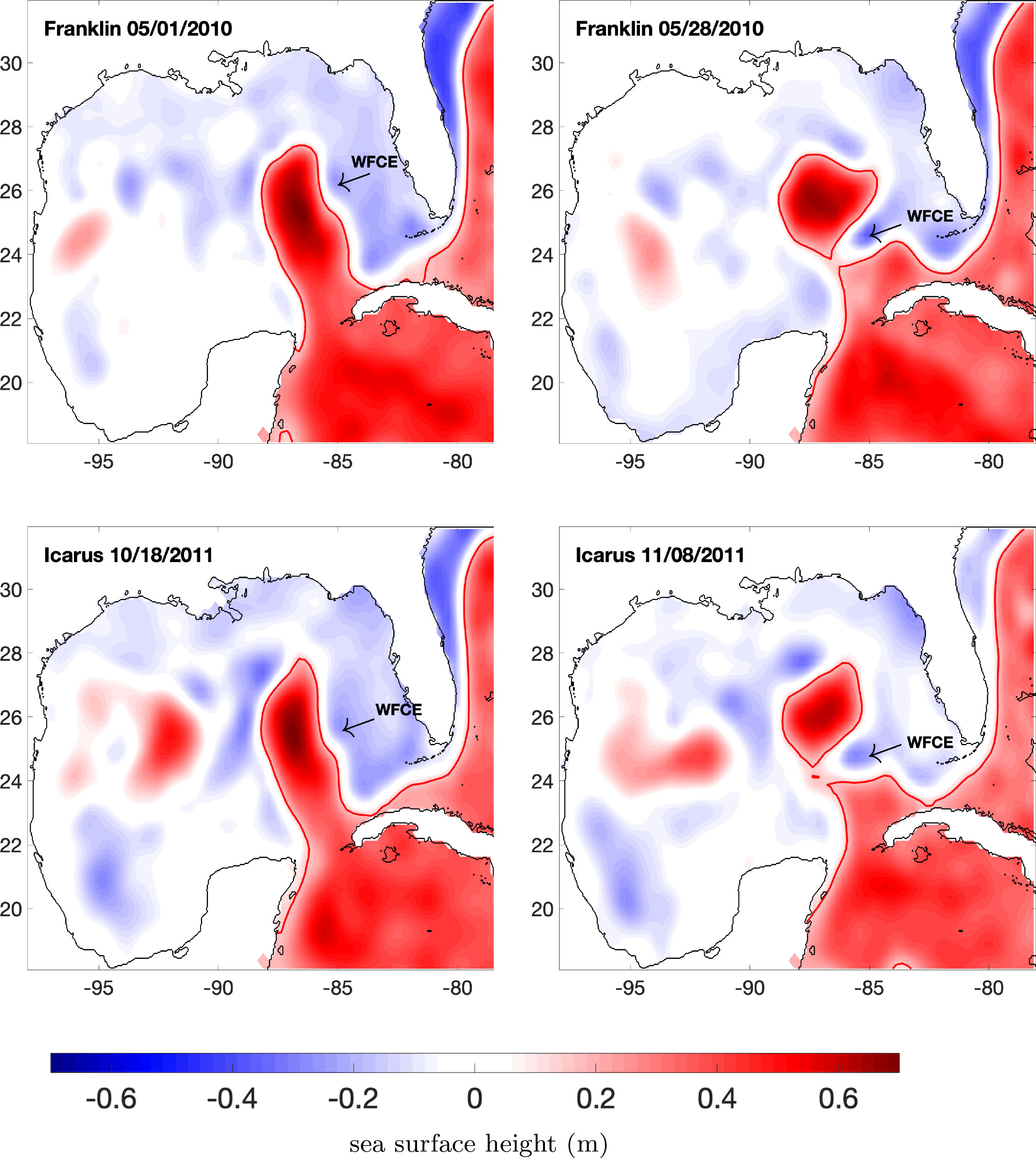
Figure 11 Altimetry-derived SSH (m) for Eddy Franklin in 2010 and Icarus in 2011. The black line is the coastline. The red line is 0.17 m SSH contour, which is the edge of the LC (Leben, 2005). The WFCE that is intruding into the LC and causing the LCE detachment is marked by an arrow and the mention “WFCE”.

3.4 Observation-model comparison

In this subsection, we compare the ensemble outputs with mooring observation data to investigate how the initial condition perturbations impact the realism of the model outputs, in light of our results from the ensemble modeling, in particular related to the detachment or not of an LCE.

To make the mooring observation and model outputs comparable in both time and space, we take the daily mean of the PE section mooring data to match the date of the daily HYCOM outputs. Then we use linear and bi-linear interpolation to interpolate the model data onto the mooring locations.

Firstly, we make model-observation comparison of the current velocity components tangential and normal to the mooring line (See Figure 1 for the locations of the mooring stations from PE1 to PE5. See Table 2 in Athie et al. (2014) for the coordinates of each PE mooring station). The comparison of the normal velocity component (normal with respect to the mooring array, i.e. along the dominant current direction) at shallow depth (50 to 60 m) for each mooring station is shown in Figure 12. In the beginning of the comparison period, the ensemble of realizations yield values that are very close to each other and generally capture the observed trend, if not the exact observed values. The ensemble starts to diverge around day 25. Apart from mooring PE5 where no model realization follows the observed trends, a subset of realizations tends to generally compare reasonably well with the observations or their trends (blue lines), while other realizations deviate from the observations (red lines). Compared to the blue realization group, the red group generally shows small variations through time, and fails to capture the characteristics of the observations. Overall, the model realizations in which an LCE detachment occurs are closer to the observations or their trend than the ones in which there is no LCE detachment. Since an LCE detachment was actually observed (Figure 10, on day 28), this comparison shows that the simulations with a strong initial WCFE, which leads to an LCE detachment, provide a reasonable representation of the early stages of the shedding process of Eddy Franklin, and that our ensemble is adapted to study the sensitivity of this process to initial conditions.

Figure 12 Comparison of model and mooring data for the normal(with respect to the mooring array) velocity U_nfor each mooring station at depth 50∼60 m. The realizations with an LCE detachment are in blue color. The realizations without an LCE detachment are in red color. The bold black lines are the observed velocities from the mooring array. The horizontal dashed line is the line of zero velocity.

We also compare the relative vorticity (RV) between the ensemble members and the mooring array observations. Due to the lack of salinity data in the moorings, it is not possible to estimate the PV. Since the mooring data are aligned on a straight line, we can only measure the across-line component of the RV $\frac{d{U}_n}{d{x}_t}$, where dU_nis the difference in normal velocities U_nbetween two adjacent mooring stations (i.e., PE1 and PE2, PE2 and PE3, etc), and dx_tis the distance between these stations. Figure 13 presents the vertical section of the RV from mooring data and from the three representative ensemble realizations on day 1. The observation exhibits high positive RV formed near the surface, over the shallow region along the CB, while the simulations all present high positive RV at depth, close to the shelf break. Figure 14 shows that the observed positive RV structure is shifted eastwards on day 25, and that this offshore displacement appears barotropic. In the simulations, the deep patch of positive RV lifts upwards and the RV structure in RZ49 has become very similar to the one in the observations. On day 30 (Figure 15), the patch of of positive RV in the observation extends eastwards at depth, and gradually becomes smaller when closer to the surface, with the core of the structure (highest RV) near the surface, over the CB shelf break. Among the three simulations, RZ49 matches with the observation very well regarding the positive RV structure. Based on SSH values, RZ49 shows an LCE that detaches on May 27th, which is very close to May 28th, the LCE actual detachment altimetry observations. This comparison confirms that the simulations in which an LCE detachment takes place, thanks to realistic initial conditions, compare well with the observations throughout the study period.

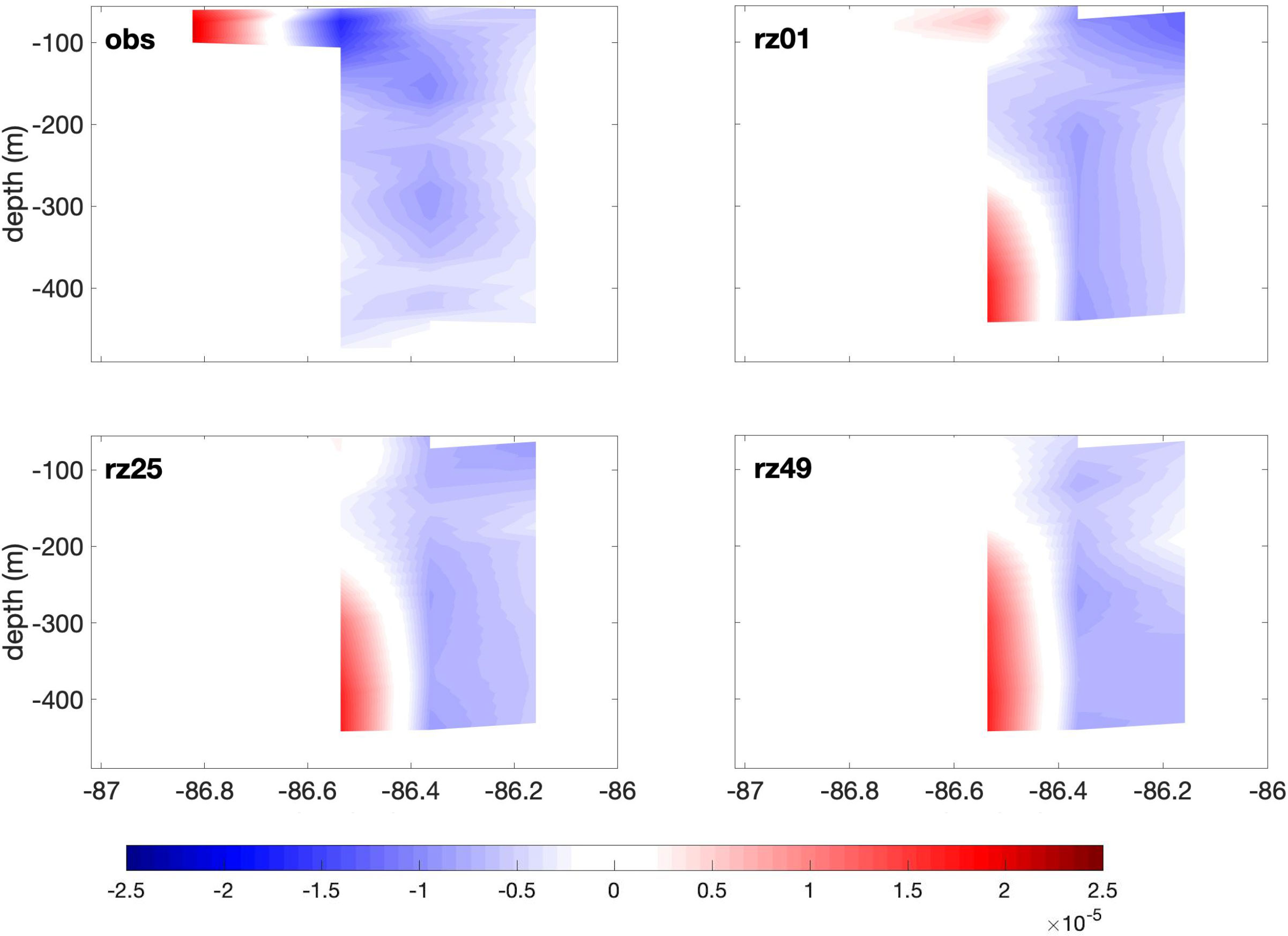
Figure 13 Vertical section of the RV (s⁻¹) over the eastern CB on day 1 for mooring data (upper left), rz 01 (upper right), rz 25 (lower left) and rz 49 (lower right).

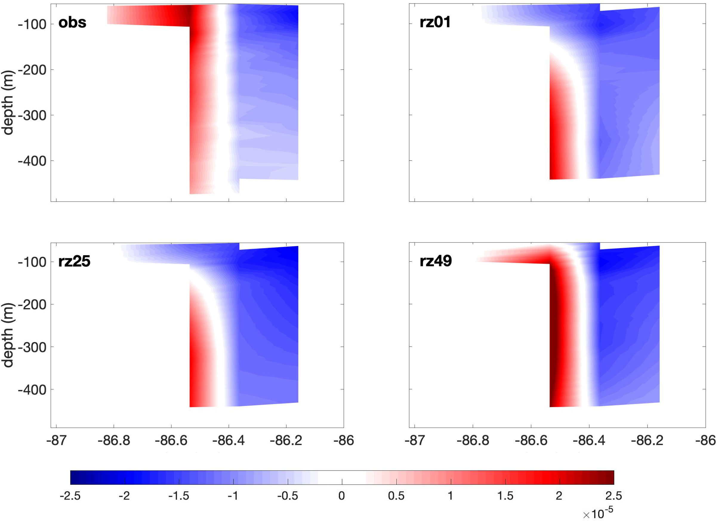
Figure 14 same as Figure 13, on day 25.

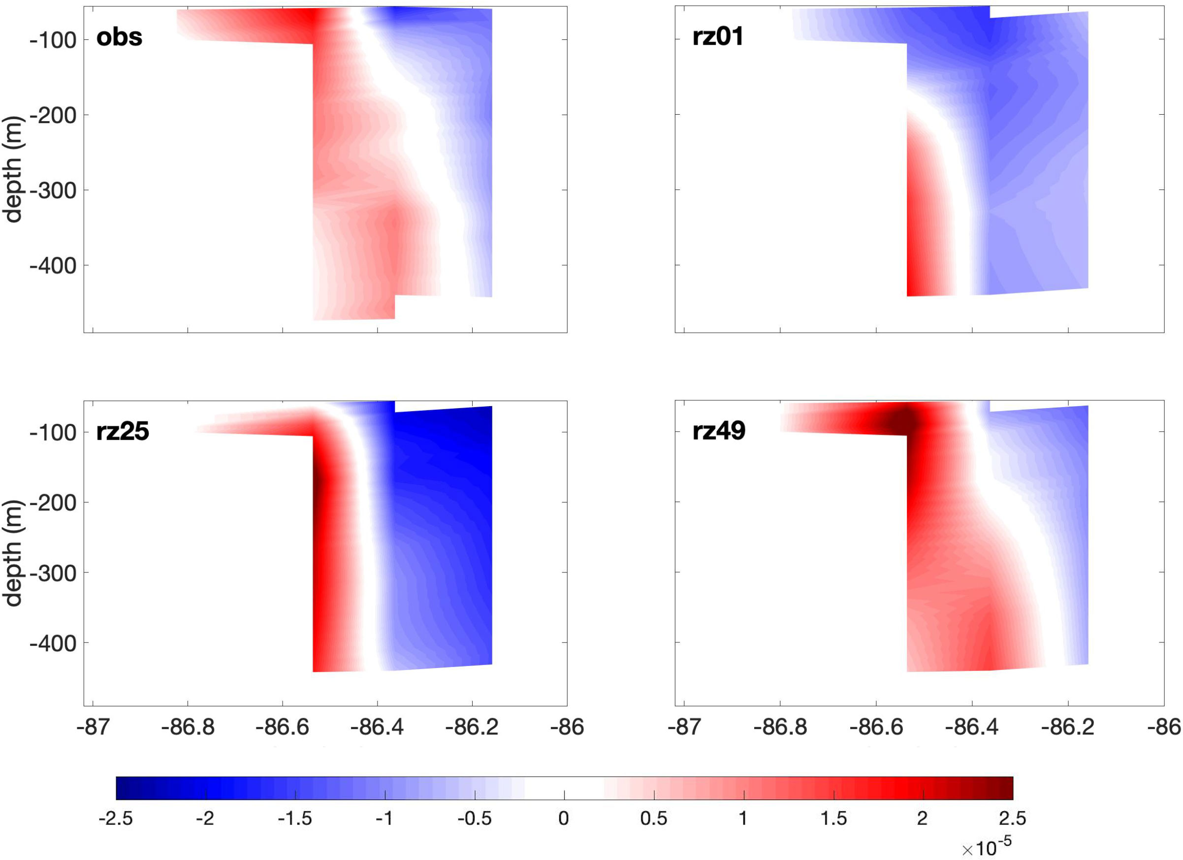
Figure 15 same as Figure 13, on day 30.

4 Summary and discussion

This paper analyses the impacts of perturbing the initial conditions in an ensemble simulation of the LC system whose main goal was forecasting the detachment of LCE Franklin. By targeting specific aspects of the initial conditions, namely the size and strength of the WFCE, the ensemble is used to investigate the dynamic impacts of such perturbations on LC detachments. The methodology adopted allowed us to build a direct relationship between two uncertain parameters controlling the initial perturbations and their subsequent impact on the ensuing LC circulation. The spatial distribution of the perturbations was obtained through an EOF decomposition of a 14-day time series of a realistic model representation of the GoM where the dominant modes reflect the variability of the LC frontal dynamics (Iskandarani et al., 2016).The two uncertain parameters, ξ₁ and ξ₂, consisted of the amplitude of the two dominant modes. _{1 2} Our research finds that both the WFCE and CBCE are perturbed by the first variability mode. More positive value of ξ₁ yields stronger WFCE immediately and stronger CBCE around 25 days later. The strong LCFEs consequently favor the detachment of an LCE. Meanwhile, the LCFEs are quite insensitive to changes in ξ_2.

This teleconnection between the CBCE and the WFCE during the LCE detachment process has been confirmed by a statistical analysis, in which we found that the PV growing on east of the CB is positively correlated with the strength of the WFCE and the distance between those PV poles. In the ensemble realizations analysis, we found that a strong WFCE leads to the formation of a CBCE, while a CBCE does not form when the WFCE weak or small. Combining those findings, we draw the conclusion that the more intense WFCE and the closer it is approaching to the CB, the more cyclonic PV will gather east of the CB. The approaching strong WFCE strengthens a forming CBCE which can subsequently intrude into the LC from its western side.

The ensemble members all share the same boundary conditions in the Caribbean Sea, so that the differences appearing in the CB region in the ensemble of simulations only come from the perturbations of the initial conditions. Considering that these perturbations are insignificant in the CB region, but that their signature is in the strength of the WFCE, the formation of a CBCE around and after day 25 can be attributed to the initial strength of the WFCE. If the formation of the CBCE was independent from the initial strength of the WFCE, the surface response of the PV amplitude in the CB region to the initial perturbation amplitudes would remain flat throughout the simulations, unlike what is seen on Figure 6. Moreover, the scatterplots relating the PV values in the CB region to the initial WFCE strength or size would show scattered values for each subplot, without pattern and without any high correlation values, unlike what is seen on Figures 8, 9. These considerations make it clear that there exists a teleconnection between the CBCE and the WFCE in our study case of the formation of Eddy Franklin. Hiron et al. (2022) revealed that during LCE detachment, some of the WFCE water originates from the outer band of the LC front. In particular, small cyclonic eddies along the northern edge of the LC were found to merge and form a larger frontal eddy on the eastern side of the LC. This is indicative of a connection between small LCFEs along the LC and the formation of a WFCE. However, that connection is directed by the advective time scales along the edge of the LC and implies physical contact (through merging), whereas in the present study the connection is remote between two distinct eddies that do not necessarily merge.

Comparing the model outputs with mooring velocity observations along the eastern CB, we found that those ensemble realizations with relatively strong initial WFCE (realizations with LCE detachment) generally capture the characteristics of the observation evolution. The high RV corresponding to the CBCE formation in the observation is first visible at the surface, while in model simulations it appears to be lifted from deep region. However, as the time increases, the simulations successfully represent the eastward displacement of the high RV structure. The realizations with an LCE detachment present positive RV structures that are quite similar to the observations after around day 25.

Another significant phenomenon that we find through this investigation is that the initial state (size and strength) of the WFCE determines the evolution of the CBCE and the occurrence of the LCE detachment around 25 days and later. A strong and large WFCE leads to an LCE detachment and the formation of a CBCE along the eastern flank of the CB. By contrast, a weak and small WFCE in the northeastern side of the LC does not trigger an LCE detachment, or the formation of a CBCE. This result is consistent with Le Hénaff et al. (2014), in which the authors show that only intense WFCEs appear to participate in LC detachments. Our results suggest that the state of the WFCE may be a predictor of the LC system evolution. The size and strength of WFCE when it’s present on the northeastern flank of the LC, can determine whether a CBCE will develop later on, and whether a LC detachment will occur or not. Moreover, since we have found that a stronger and larger initial WFCE leads to an earlier LCE detachment date (Figure 10), it might be possible to estimate the approximate date of an upcoming LCE detachment, after a well-formed WFCE is identified on the northeastern flank of the LC with a measurement of its size or strength. This suggestion is based on the study case of the formation of Eddy Franklin, but the sequence of eddy presence observed in our study case at the beginning of the shedding process was observed in the shedding process of Eddy Icarus, which followed Eddy Franklin in 2011, and is more generally consistent with the descriptive study of Schmitz (2005). In addition, Sheinbaum et al. (2016) mentioned that, for certain LCE detachments, the strength of the CBCE matches that of the WFCE, unlike during the Eddy Franklin shedding; it is worthwhile to investigate to what extent the teleconnection between LCFEs identified in our study is preserved under the latter scenario. Further research needs to be conducted on multiple LCE detachment events, in order to construct and test a valid relationship between the WFCE state and the LCE detachment process.

Author’s note

The content is solely the responsibility of the authors and does not necessarily represent the official views of the Gulf Research Program or the National Academies of Sciences, Engineering, and Medicine.

Data availability statement

The raw data supporting the conclusions of this article will be made available by the authors, without undue reservation.

Author contributions

XY, MI and MLH conceived of the presented idea. XY and MLH performed the computations. MI supervised the findings of this work. XY, MI and MLH analyzed the results from the investigation and made conclusions. BM provides suggestions during the conduction of the investigation. XY wrote the paper with comments from all other authors. All authors contributed to the article and approved the submitted version.

Funding

This research was made possible by the support of the National Science Foundation Award 1639722 and ONR grant N000141912671. MLH received partial support for work on this publication by NOAA/AOML and was supported in part under the auspices of the Cooperative Institute for Marine and Atmospheric Studies (CIMAS), a cooperative institute of the University of Miami and NOAA (agreement NA20OAR4320472). Research reported in this publication was partially supported by the Gulf Research Program of the National Academies of Sciences, Engineering, and Medicine under the Grant Agreement number 2000011056 and the Grant Agreement number 2000013149.

Acknowledgments

The mapped altimetry products were produced by Ssalto/Duacs and distributed by the Copernicus Marine Environment Marine Service.

Conflict of interest

The authors declare that the research was conducted in the absence of any commercial or financial relationships that could be construed as a potential conflict of interest.

Publisher’s note

All claims expressed in this article are solely those of the authors and do not necessarily represent those of their affiliated organizations, or those of the publisher, the editors and the reviewers. Any product that may be evaluated in this article, or claim that may be made by its manufacturer, is not guaranteed or endorsed by the publisher.

Abbreviations

*Fully documented templates are available in the elsarticle package on CTAN.

Footnotes

1. ^ For the detailed information of these LCEs, please see the Woods Hole Gulf of Mexico Loop Current Eddies records website: https://www.horizonmarine.com/loop-current-eddies.
2. ^ The details of the model configuration, including advection scheme, mixing, vertical structure, can be found in the HYCOM website: https://www.hycom.org/data/goml0pt04/expt-20pt1
3. ^ To access COAMPS model code and data, please see https://cordc.ucsd.edu/projects/models/coamps/.
4. ^ The sampling was designed to minimize the error between a Polynomial Chaos surrogate and the sample via a Galerkin projection on polynomials of degree 6 in the variables ξ₁ and ξ₂. See Figure 3 in Iskandarani et al. (2016) for the sampling points in the uncertain (ξ₁,ξ₂) space.
5. ^ The ensemble standard deviation were calculated using the Polynomial Chaos surrogate, see Le Maı̂tre and Knio (2010) and Iskandarani et al. (2016) for details.

References

Androulidakis Y., Kourafalou V., Le Hénaff M., Kang H., Ntaganou N. (2021). The role of mesoscale dynamics over northwestern Cuba in the loop current evolution in 2010, during the deepwater horizon incident. J. Mar. Sci. Eng. 9, 1–26. doi: 10.3390/jmse9020188
Androulidakis Y., Kourafalou V. H., Le Hénaff M. (2014). Influence of frontal cyclone evolution on the 2009 (ekman) and 2010 (franklin) loop current eddy detachment events. Ocean Sci. 10, 947–965. doi: 10.5194/os-10-947-2014
Athié G., Candela J., Ochoa J., Sheinbaum J. (2012). Impact of caribbean cyclones on the detachment of loop current anticyclones. J. Geophysical Research: Oceans 117. doi: 10.1029/2011JC007090
Athie G., Sheinbaum J., Romero A., Ochoa J., Candela J. (2014). “Measurements in the Yucatan-Campeche area in support of the Loop Current dynamics study,” in Technical Report, Bureau of Ocean Energy Management, Gulf of Mexico OCS Region, New Orleans. (New Orleans, Louisiana: United States. Department of the Interior), 159pp.
Bao J., Wilczak J., Choi J., Kantha L. (2000). Numerical simulations of air–sea interaction under high wind conditions using a coupled model: A study of hurricane development. Monthly Weather Rev. 128, 2190–2210. doi: 10.1175/1520-0493(2000)128<2190:NSOASI>2.0.CO;2
Bleck R. (2002). An oceanic general circulation model framed in hybrid isopycnic-cartesian coordinates. Ocean Model. 4, 55–88. doi: 10.1016/S1463-5003(01)00012-9
Candela J., Sheinbaum J., Ochoa J., Badan A., Leben R. (2002). The potential vorticity flux through the yucatan channel and the loop current in the gulf of Mexico. Geophysical Res. Lett. 29, 16–11. doi: 10.1029/2002GL015587
Candela J., Tanahara S., Crepon M., Barnier B., Sheinbaum J. (2003). Yucatan channel flow: Observations versus clipper atl6 and mercator pam models. J. Geophysical Research: Oceans 108. doi: 10.1029/2003JC001961
Chang Y.-L., Oey L.-Y. (2011). Loop current cycle: coupled response of the loop current with deep flows. J. Phys. Oceanography 41, 458–471. doi: 10.1175/2010JPO4479.1
Chassignet E. P., Hurlburt H. E., Smedstad O. M., Halliwell G. R., Hogan P. J., Wallcraft A. J., et al. (2007). The hycom (hybrid coordinate ocean model) data assimilative system. J. Mar. Syst. 65, 60–83. doi: 10.1016/j.jmarsys.2005.09.016
Chassignet E. P., Smith L. T., Halliwell G. R., Bleck R. (2003). North atlantic simulations with the hybrid coordinate ocean model (hycom): Impact of the vertical coordinate choice, reference pressure, and thermobaricity. J. Phys. Oceanography 33, 2504–2526. doi: 10.1175/1520-0485(2003)033<2504:NASWTH>2.0.CO;2
Cherubin L. M., Sturges W., Chassignet E. P. (2005). Deep flow variability in the vicinity of the yucatan straits from a high-resolution numerical simulation. J. Geophysical Research-Oceans 110, C04009. doi: 10.1029/2004JC002280
Cochrane J. D. (1972). Separation of an anticyclone and subsequent developments in the loop current (1969). Contributions Phys. Oceanography Gulf Mexico 2, 91–106.
Fratantoni P. S., Lee T. N., Podesta G. P., Muller-Karger F. (1998). The influence of loop current perturbations on the formation and evolution of tortugas eddies in the southern straits of florida. J. Geophysical Research: Oceans 103, 24759–24779. doi: 10.1029/98JC02147
Halliwell G. R. (2004). Evaluation of vertical coordinate and vertical mixing algorithms in the hybrid-coordinate ocean model (hycom). Ocean Model. 7, 285–322. doi: 10.1016/j.ocemod.2003.10.002
Hamilton P., Lugo-Fern´andez A., Sheinbaum J. (2016). A loop current experiment: Field and remote measurements. Dynamics Atmospheres Oceans 76, 156–173. doi: 10.1016/j.dynatmoce.2016.01.005
Herbette S., Morel Y., Arhan M. (2005). Erosion of a surface vortex by a seamount on the β plane. J. Phys. oceanography 35, 2012–2030. doi: 10.1175/JPO2809.1
Hiron L., de la Cruz B. J., Shay L. K. (2020). Evidence of loop current frontal eddy intensification through local linear and nonlinear interactions with the loop current. J. Geophysical Research: Oceans 125, e2019JC015533. doi: 10.1029/2019JC015533
Hiron L., Miron P., Shay L. K., Johns W. E., Chassignet E. P., Bozec A. (2022). Lagrangian coherence and source of water of loop current frontal eddies in the gulf of Mexico. Prog. Oceanography 208, 102876. doi: 10.1016/j.pocean.2022.102876
Hoskins B. J., McIntyre M. E., Robertson A. W. (1985). On the use and significance of isentropic potential vorticity maps. Q. J. R. Meteorological Soc. 111, 877–946. doi: 10.1002/qj.49711147002
Hurlburt H. E., Thompson J. D. (1982). The dynamics of the loop current and shed eddies in a numerical model of the gulf of Mexico. Elsevier Oceanography Ser. 34, 243–297. doi: 10.1016/S0422-9894(08)71247-9
Iskandarani M., Le Hénaff M., Thacker W. C., Srinivasan A., Knio O. M. (2016). Quantifying uncertainty in gulf of Mexico forecasts stemming from uncertain initial conditions. J. Geophysical Research: Oceans 121, 4819–4832. doi: 10.1002/2015JC011573
Jaimes B., Shay L. K., Uhlhorn E., Cook T. M., Brewster J., Halliwell G., et al. (2006). Influence of loop current ocean heat content on Hurricanes Katrina, Rita, and Wilma. In Proceedings of the 27th Conference on Hurricanes and Tropical Meteorology. (Monterey, CA, USA), 24–28.
Leben R. R. (2005). Altimeter-derived loop current metrics. Geophysical Monograph-American Geophysical Union 161, 181. doi: 10.1029/161GM15
Le Hénaff M., Kourafalou V. H., Androulidakis Y., Ntaganou N., Kang H. (2023). Influence of the caribbean sea eddy field on loop current predictions. Front. Mar. Sci. 10, 1129402. doi: 10.3389/fmars.2023.1129402
Le Hénaff M., Kourafalou V. H., Dussurget R., Lumpkin R. (2014). Cyclonic activity in the eastern gulf of Mexico: Characterization from alongtrack altimetry and in situ drifter trajectories. Prog. Oceanography 120, 120–138. doi: 10.1016/j.pocean.2013.08.002
Le Hénaff M., Kourafalou V. H., Morel Y., Srinivasan A. (2012a). Simulating the dynamics and intensification of cyclonic loop current frontal eddies in the gulf of Mexico. J. Geophysical Research: Oceans 117. doi: 10.1029/2011JC007279
Le Hénaff M., Kourafalou V. H., Paris C. B., Helgers J., Aman Z. M., Hogan P. J., et al. (2012b). Surface evolution of the deepwater horizon oil spill patch: combined effects of circulation and wind-induced drift. Environ. Sci. Technol. 46, 7267–7273. doi: 10.1021/es301570w
Le Maître O., Knio O. M. (2010). Spectral methods for uncertainty quantification: with applications to computational fluid dynamics (Berlin: Springer Science & Business Media).
Li G., Iskandarani M., Le Hénaff M., Winokur J., Le Maˆıtre O. P., Knio O. M. (2016). Quantifying initial and wind forcing uncertainties in the gulf of Mexico. Comput. Geosciences 20, 1133–1153. doi: 10.1007/s10596-016-9581-4
Liu Y., Weisberg R. H., Hu C., Zheng L. (2011). Tracking the deepwater horizon oil spill: A modeling perspective. Eos Trans. Am. Geophysical Union 92, 45–46. doi: 10.1029/2011EO060001
McDonald M. (2006) Hycom + ncoda gulf of Mexico 1/25° analysis (goml0.04/expt 20.1). Available at: http://https://www.hycom.org/data/goml0pt04.
Meunier T., Rossi V., Morel Y., Carton X. (2010). Influence of bottom topography on an upwelling current: Generation of long trapped filaments. Ocean Model. 35, 277–303. doi: 10.1016/j.ocemod.2010.08.004
Mezić I., Loire S., Fonoberov V. A., Hogan P. (2010). A new mixing diagnostic and gulf oil spill movement. Science 330, 486–489. doi: 10.1126/science.1194607
National Academies of Sciences, et al. (2018). Understanding and predicting the gulf of Mexico loop current: critical gaps and recommendations (Washington, DC: National Academies Press). doi: 10.17226/24823
Ntaganou N., Kourafalou V., Beron-Vera F. J., Olascoaga M. J., Le Hénaff M., Androulidakis Y. (2023). Influence of caribbean eddies on the loop current system evolution. Front. Mar. Sci. 10, 961058. doi: 10.3389/fmars.2023.961058
Oey L.-Y. (2004). Vorticity flux through the yucatan channel and loop current variability in the gulf of Mexico. J. Geophysical Research-Oceans 109. doi: 10.1029/2004JC002400
Oey L.-Y. (2008). Loop current and deep eddies. J. Phys. Oceanography 38, 1426–1449. doi: 10.1175/2007JPO3818.1
Pichevin T., Nof D. (1997). The momentum imbalance paradox. Tellus 49A, 298–319. doi: 10.3402/tellusa.v49i2.14484
Schmitz J. W.J. (2003). “Notes on the circulation in and around the gulf of Mexico,” in A review of the deep water circulation, vol. i. (TX, USA: Texas A&M University Press, College Station).
Schmitz J. W.J. (2005). Cyclones and westward propagation in the shedding of anticyclonic rings from the loop current. Washington DC Am. Geophysical Union Geophysical Monograph Ser. 161, 241–261. doi: 10.1029/161GM18
Sheinbaum J., Athi´e G., Candela J., Ochoa J., Romero-Arteaga A. (2016). Structure and variability of the yucatan and loop currents along the slope and shelf break of the yucatan channel and campeche bank. Dynamics Atmospheres Oceans 76, 217–239. doi: 10.1016/j.dynatmoce.2016.08.001
Sturges W., Evans J. (1983). On the variability of the loop current in the gulf of Mexico. J. Mar. Res. 41, 639–653. doi: 10.1357/002224083788520487
Sturges W., Hoffmann N. G., Leben R. R. (2010). A trigger mechanism for loop current ring separations. J. Phys. Oceanography 40, 900–913. doi: 10.1175/2009JPO4245.1
Valentine D. L., Mezi´c I., Ma´ceˇsi´c S., Crnjari´c-ˇ Zic,ˇ N., Ivi´c S., Hogan P. J., et al. (2012). Dynamic autoinoculation and the microbial ecology of a deep water hydrocarbon irruption. Proc. Natl. Acad. Sci. 109, 20286–20291. doi: 10.1073/pnas.1108820109
Vukovich F. M., Maul G. A. (1985). Cyclonic eddies in the eastern gulf of Mexico. J. Phys. Oceanography 15, 105–117. doi: 10.1175/1520-0485(1985)015<0105:CEITEG>2.0.CO;2
Walker N. D., Pilley C. T., Raghunathan V. V., D’Sa E. J., Leben R. R., Hoffmann N. G., et al. (2011). Impacts of loop current frontal cyclonic eddies and wind forcing on the 2010 gulf of Mexico oil spill. Monit. Modeling Deepwater Horizon Oil Spill: A Record-Breaking Enterprise 195, 103–116. doi: 10.1029/2011GM001120
Wang S., Li G., Iskandarani M., Le Hénaff M., Knio O. M. (2018). Verifying and assessing the performance of the perturbation strategy in polynomial chaos ensemble forecasts of the circulation in the gulf of Mexico. Ocean Model. 131, 59–70. doi: 10.1016/j.ocemod.2018.09.002
Keywords: Loop Current, ensemble simulations, Campeche Bank cyclonic eddy, West Florida cyclonic eddy, potential vorticity, teleconnection
Citation: Yang X, Le Hénaff M, Mapes B and Iskandarani M (2023) Dynamical interactions between Loop Current and Loop Current Frontal Eddies in a HYCOM ensemble of the circulation in the Gulf of Mexico. Front. Mar. Sci. 10:1048780. doi: 10.3389/fmars.2023.1048780
Received: 20 September 2022; Accepted: 13 September 2023;
Published: 13 October 2023.
Edited by:
Julio Sheinbaum, Centro de Investigación Científica y de Educación Superior de Ensenada (CICESE), MexicoReviewed by:
Wei Huang, Oak Ridge National Laboratory (DOE), United StatesJorge Zavala-Hidalgo, Universidad Nacional Autónoma de México, Mexico
Efrain Moreles, National Autonomous University of Mexico, Mexico
Copyright © 2023 Yang, Le Hénaff, Mapes and Iskandarani. This is an open-access article distributed under the terms of the Creative Commons Attribution License (CC BY). The use, distribution or reproduction in other forums is permitted, provided the original author(s) and the copyright owner(s) are credited and that the original publication in this journal is cited, in accordance with accepted academic practice. No use, distribution or reproduction is permitted which does not comply with these terms.
*Correspondence: Xingchen Yang, xxy181@miami.edu