Chlorophyll response to wind and terrestrial nitrate in the western and southern continental shelves of the Gulf of Mexico

1 Introduction

The Gulf of Mexico (GoM or gulf hereafter) is a semi-enclosed sea that covers an area of ∼ 1.5 × 10⁶ km². It is located between 18–30° N and 82–98° W (Figure 1) and connects with the Atlantic Ocean through the Yucatan Channel and the Straits of Florida. The general circulation of the GoM is driven by the Loop Current, which enters the gulf through the Yucatan Channel. The Loop Current, as its name suggests, forms an anticyclonic semi-closed loop after it enters the gulf before exiting through the Straits of Florida. Anticyclonic mesoscale eddies detach from the Loop Current and propagate westward with speeds of ∼2 km per day (Elliott, 1982). Vázquez De La Cerda et al. (2005) established that a semi-permanent cyclonic' eddy forced by Ekman pumping associated with wind stress curl is present in the Bay of Campeche (BOC), which is located in the southern region of the GoM.

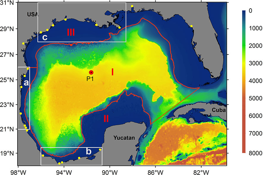
Figure 1 Gulf of Mexico bathymetry (m) and model domain. The yellow dots represent the rivers used in the model configuration. The red line represents the 200 m isobath that divides the gulf into three major regions: the deep region (I), southern coastal region (II), and northern coastal region (III). The areas within gray boxes represent the Tamaulipas-Veracruz (TAVE; (A), Bay of Campeche (BOC; (B) and Louisiana-Texas (LATEX; (C) shelves, respectively. TAVE and BOC areas were used to calculate daily chlorophyll, wind, and nitrate flux means.

The advection of low salinity water and coastal upwelling are among the relevant processes associated with wind seasonality. Coastal upwelling due to Ekman transport occurs in summer and winter in the southern and northern regions of the gulf, respectively (Zavala-Hidalgo et al., 2003; Zavala-Hidalgo et al., 2006). During the fall and winter, low salinity waters arrive from the Mississippi and Atchafalaya rivers and the Louisiana-Texas (LATEX) platform to the Tamaulipas-Veracruz (TAVE) platform. During the summer, water is advected over the continental shelf from the TAVE to LATEX region. Of the 16 rivers that flow into the GoM from Mexican territory, the Grijalva, Usumacinta, Coatzacoalcos, Papaloapan, and Panuco rivers provide the majority of the freshwater to the gulf, with a combined flow of ∼ 2.2 × 10⁶ m³ per year (Figure 2). This value constitutes ∼ 90% of the total runoff from Mexican territory into the GoM (CONAGUA, 2014). Together with contributions from the United States, this fluvial runoff promotes the formation of large regions in which the primary productivity has a seasonal component that is strongly linked to nitrogen-rich freshwater inputs (Lohrenz et al., 1997; Fennel et al., 2011; Nababan et al., 2011). The information available on the nutrient content and flow of these large continental fluvial inputs is either scarce or intermittent. More importantly, measurements have often been taken in the regions of the continental basins and not in the river mouths where information on net flow is needed to calculate the discharge and total nitrate flowing from the basins to the ocean.

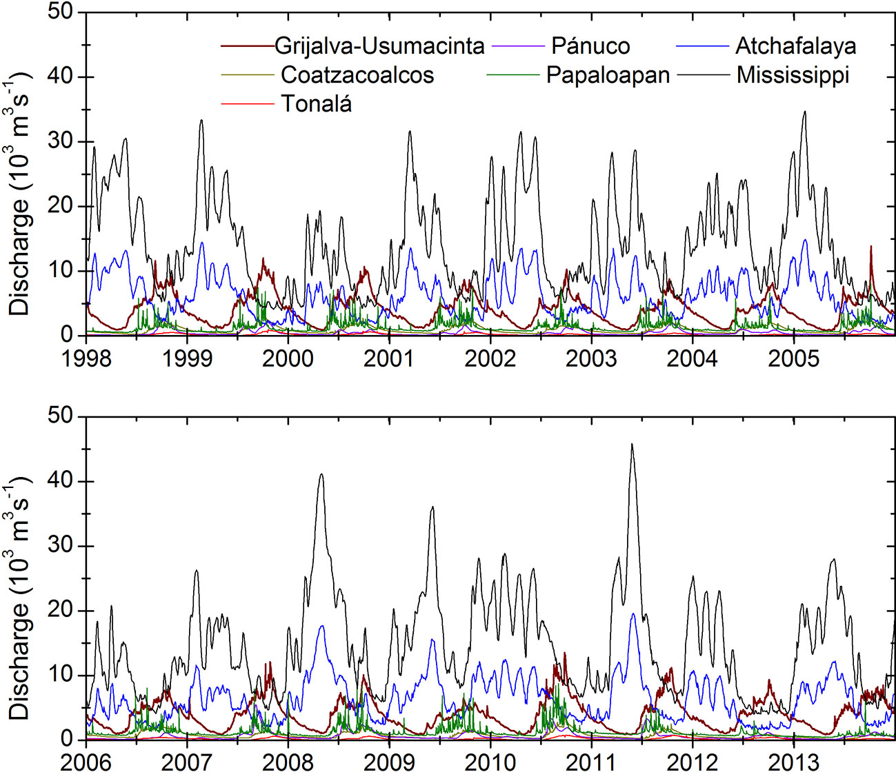
Figure 2 Observed (Mississippi and Atchafalaya) and simulated (Grijalva-Usumacinta, Coatzacoalcos, Tonala, Panuco and Papaloapan) major river discharges used in the model. Seven out of 24 of the implemented rivers are shown.

In the present study, we used a hydrodynamic model coupled to a biogeochemical model to simulate the main physical and biogeochemical features of the GoM emphasizing the influence of wind and rivers on the chlorophyll dynamics over the continental shelf. We used as river forcing the simulated data reported by González-Ramírez and Parés-Sierra (2019). In such study, the authors concluded that the flow and nutrient ´ data of rivers that flow towards the GoM have been underestimated in some of the Mexican rivers, the main and most evident being the Grijalva-Usumacinta system.

We compare surface chlorophyll time series to river discharge and wind records to evaluate the main drivers of chlorophyll variability in the TAVE and BOC regions. Then, using a spectral and Empirical Orthogonal Functions (EOFs) analysis, we describe the principal modes of surface chlorophyll variability in model results and satellite observations.

2 Model configuration

2.1 Physical model

For this study, we used the Coastal and Regional Ocean COmmunity model (CROCO) v. 1.0 (Debreu et al., 2012) to simulate the physical processes of the GoM for the 21 year period between 1993 and 2013. The model domain included the entire GoM from 79.30–98.00° W and from 18.10–30.70° N. The model was configured with a 1/20° horizontal resolution, 40 terrain-following vertical levels, and 3 min time steps. The model employed a third-order upstream-rotated advection scheme, third-order upstream advection of momentum, and the non-local K-profile (Large et al., 1994) closure scheme for vertical turbulent mixing. The temperature and salinity initial conditions used by the model came from the GLORYS (Global Ocean Reanalysis) Project (Lellouche et al., 2013). Our model was forced with monthly momentum means obtained from the GLORYS Project (Lellouche et al., 2013), monthly climatologies of heat and salt fluxes from the Comprehensive Ocean Atmosphere Data Set (Woodruff et al., 1987), and 6 h wind stress derived from the National Centers for Environmental Prediction (NCEP) Climate Forecast System Reanalysis (CFSR; Saha et al. (2010)) for 1998–2010 and the NCEP Climate Forecast System v. 2 [CFSv2; Saha et al. (2014)] for 2011–2013.

2.2 Biogeochemical model

The physical model was coupled with a biogeochemical model (Gruber et al., 2006), which solves the nitrogen cycle using seven state variables [i.e., nitrate (NO3); ammonium (NH4); phytoplankton (Phy); chlorophyll (Chl); zooplankton (Zoo); and two groups of detritus, namely large (LDet) and small particles (SDet)]. In the biogeochemical model, a biological boundary condition was implemented in the bottom that was similar to the one proposed by Fennel et al. (2006). The boundary condition resolves the transformation process of organic matter that reaches the bottom, which was composed of detritus and phytoplankton in this case. This organic matter is instantly remineralized into ammonium. The mathematical expression that defines this process is shown in equation 1:

where $Hz$ is the thickness of the bottom layer, 4/16 is a stoichiometric ratio where 4 moles of NH4 are produced from every 16 moles of nitrogen in the bottom, as organic matter is assumed to follow the Redfield ratio. $Phy{|}_{z=H}$, $SDet{|}_{z=H}$ and $LDet{|}_{z=H}$ are the amounts of phytoplankton, small detritus, and large detritus in the bottom layer and its corresponding sinking velocities: $w_{Phy}$, $w_{SDet}$ and $w_{LDet}$.

In order to evaluate the biogeochemical response to the contribution of nitrate from the rivers, we implemented two model configurations, namely rivers on (Rv) and rivers off (NRv). In the Rv model configuration, 24 major rivers (13 in Mexico and 11 in the United States), including their discharge, water temperature, and nitrate and ammonia concentrations (Figures 2, 3) were implemented as daily freshwater inputs. For the Usumacinta, Grijalva, Tonala, Papaloapan, Coatzacoalcos, and Panuco rivers in Mexico we used the data simulated by González-Ramírez and Parés-Sierra (2019). For the Mississippi and Atchafalaya rivers we used data measured by the US Army Corps of Engineers at Tabert Landing and Simmesport, respectively. For the remaining rivers in both Mexico and the United States, daily climatologies were calculated from the available periods. These data were retrieved from the BANDAS data base and the United States Geological Survey (USGS) respectively. For the initial biological boundary conditions, NO3 and NH4 data from the World Ocean Atlas (Boyer et al., 2013) were used. All Biological parameters used to conduct this study are shown in Table 1.

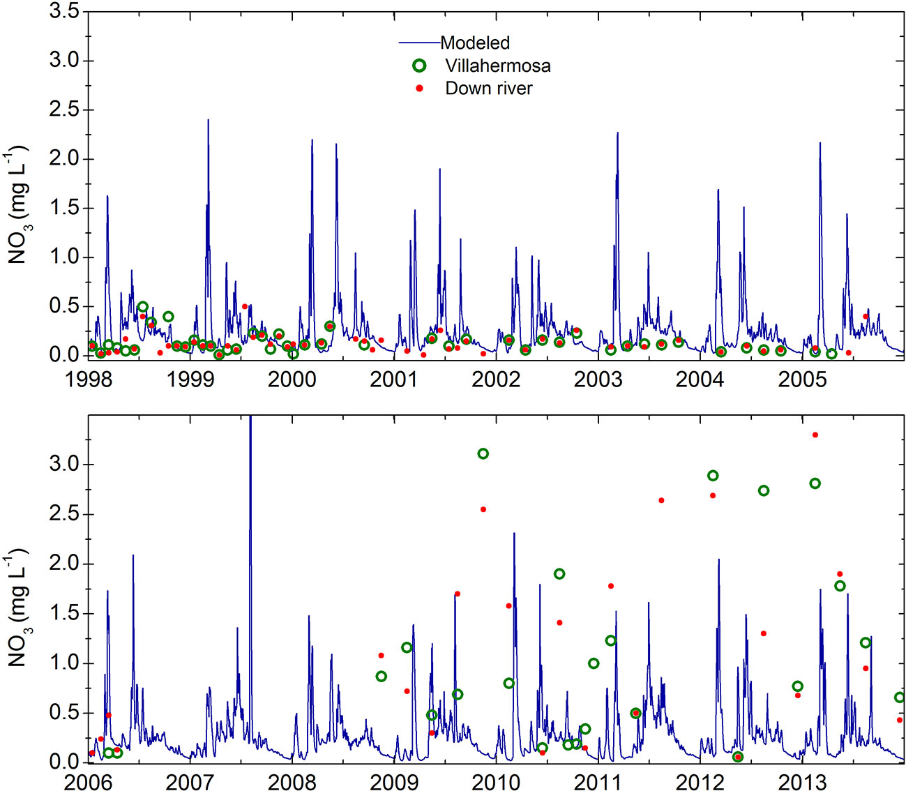
Figure 3 Simulated nitrate concentrations in the Grijalva-Usumacinta river system (blue line) from González-Ramírez and Parés-Sierra (2019) used in the model configuration. Red dots and green circles represent nitrate concentration observations in two different locations: Estacíon 16 y 42: Río Usumacinta and Estacion 3 y 4: Río Grijalva. Data obtained from SERNAPAM, Tabasco.

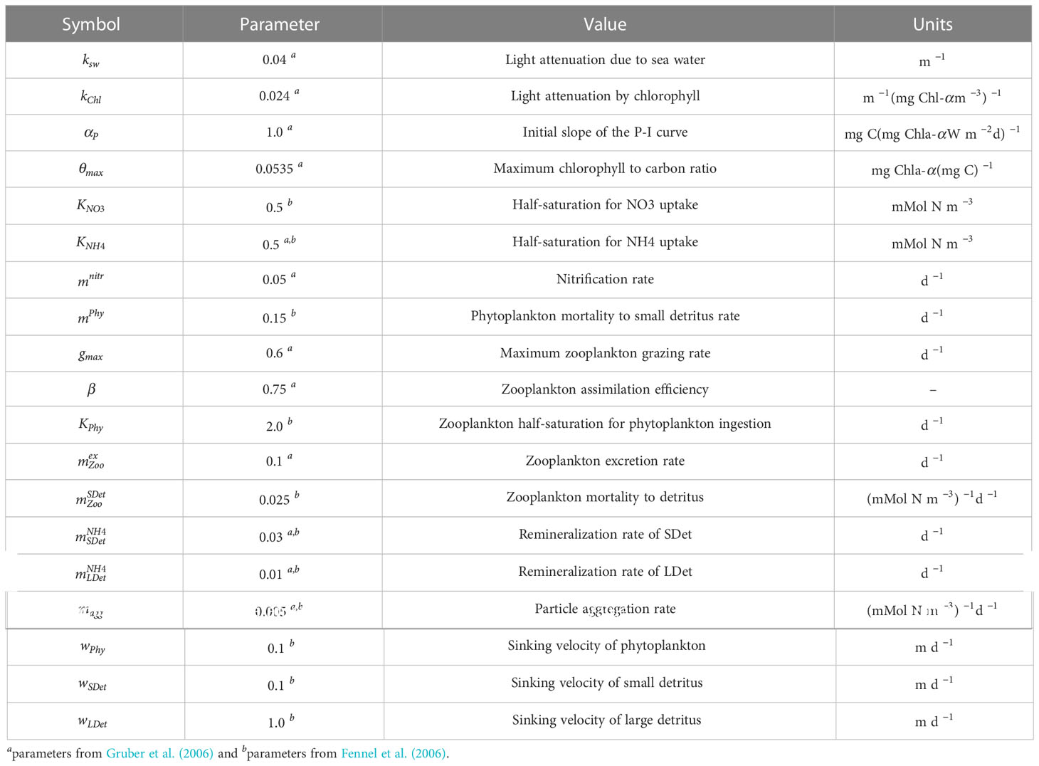
Table 1 Biogeochemical model parametrization used in this study.

3 Analysis

After conducting the 21 year simulation of the physical-biogeochemical model, we proceeded to validate the model outputs. For the biological component of the model we used the chlorophyll concentration as validation and analysis variable. As observed data, in the present study we used the monthly surface chlorophyll concentration for the period between 2003 to 2013 produced by the Moderate Resolution Imaging Spectroradiometer (MODIS) sensor with a 4 km horizontal resolution.

For the purposes of comparing observed and simulated concentrations of chlorophyll at the surface (see Figure 4), the gulf was divided into three large regions delimited by the 200 m isobath: the deep region (I) which is, the southern coastal region (II), and the northern coastal region (III) (Figure 1). Both region II and III divided at the mouth of the Rio Grande and delimited by the 200 m isobath covering all the GoM continental shelf.

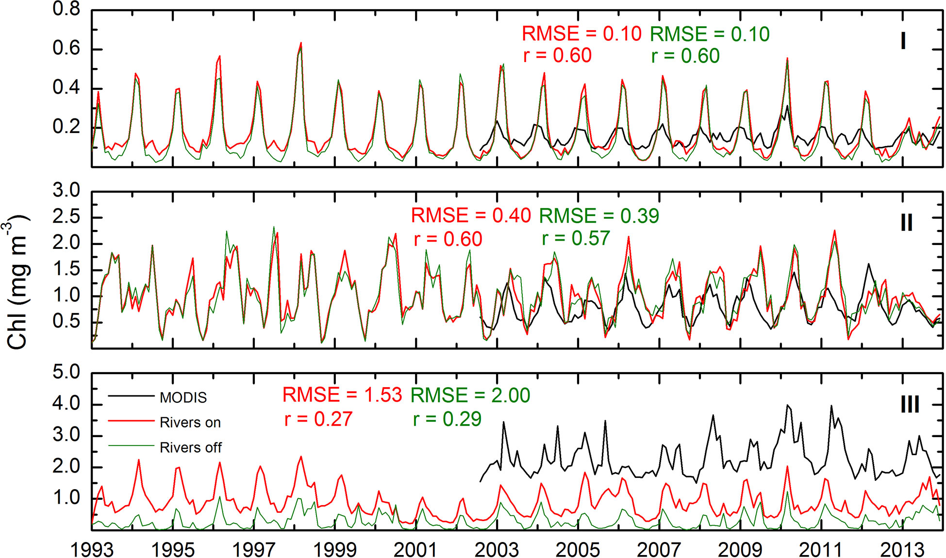
Figure 4 Monthly mean surface chlorophyll concentration. The lines represent the observed data (black) and simulated from both configurations: rivers on (red) and rivers off (green) for the deep (I), southern (II) and northern (III) regions (Figure 1). Root mean square errors and correlations factors between observed and simulated data are shown in each panel.

Regarding the vertical distribution of chlorophyll, daily sampling from 0–250 m depth was carried out at point P1 (Figure 1) during the 21 year simulation. The latter, in order to evaluate the performance of the model to correctly reproduce the chlorophyll distribution and concentration in the water column.

In order to perform a more detailed analysis in the areas (TAVE and BOC, Figure 1) in which the new data from Mexican rivers were implemented as forcings, we calculated daily averages of the upwelling-favorable wind component (Figures 5A, B), surface chlorophyll concentration from both model configurations (Figures 5C, D), and nitrate fluxes ($N{O}_{3}flux=Discharge\times N{O}_{3}concentration$) (Figures 5E, F).

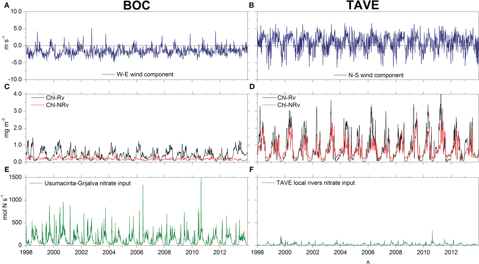
Figure 5 (A, B) - CFSR 8-day, low-pass filtered W-E(N-S) wind component for the BOC(TAVE) region. Negative(Positive) values indicate upwelling-favorable winds. (C, D) - Average daily surface chlorophyll concentrations for the BOC(TAVE) region from both model configurations Rv and NRv. (E, F) - Nitrate flux entering the BOC(TAVE) region.

Moreover, to better understand the time scales in which the different processes occur in the TAVE and BOC regions and the mechanisms associated with them, we conducted a Squared Spectral Coherence (coherence) analysis using the following equation:

where $G_x(f)$ and $G_y(f)$ are the power spectral density functions of $x(t)$ and $y(t)$, respectively, and $G_{xy}(f)$ is the cross-spectral density function between $x(t)$ and $y(t)$. The coherence express the degree of association between the phases and amplitudes of two time series and will always satisfy $0\le {\gamma }_{xy}^2\le 1$. The peaks in the coherence spectrum indicate frequencies at which the studied processes are more correlated and will be zero when the two signals are independent ofeach other (Wang and Tang, 2004; Biltoft and Pardyjak, 2009). First, we calculated the coherence between the simulated surface chlorophyll concentration ($Chl$) and the upwelling-favorable wind component ($wind$) (Figures 6A, B). Additionally, the coherence between the nitrate flux ($N{O}_{3}flux$) entering each region and the difference of surface chlorophyll from both model configurations ($\text{Δ}Chl=Ch{l}_{Rv}-Ch{l}_{NRv}$) (Figures 6C, D) was also calculated.

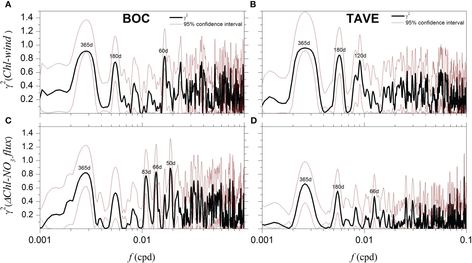
Figure 6 (A, B) - Coherence between the daily surface chlorophyll concentration from the Rv model configuration and the upwelling favorable winds in the BOC(TAVE) region. (C, D) - Coherence between the difference of daily surface chlorophyll concentration from both model configurations ($\Delta Chl$) and the nitrate flux ($N{O}_{3}flux$) from rivers for the BOC(TAVE) region.

Furthermore, from the daily data of surface chlorophyll concentration obtained from the Rv model configuration, we calculated monthly averages for the TAVE and BOC regions (Figures 1A, B). Subsequently, chlorophyll concentration anomalies were used to calculate the EOFs and their corresponding principal components (PC). The first three modes of the EOFs were calculated for the period of 1998–2013. To compare the results of the model with the available observations, the same procedure was followed with the monthly satellite images from MODIS for the period of 2003–2013. In order to identify and associate the variability peaks in the PC with atmospheric and hydrological processes, in TAVE we calculated the anomalies of the monthly N-S wind component and the Mississippi River discharge. In BOC the same was done for the W-E wind component and the Grijalva-Usumacinta river system. Then, we compare the PC from the model and observations in each region with the monthly averaged $\text{Δ}Chl$ and the aforementioned anomalies.

4 Results and discussion

Both configurations of our model were capable of representing the main physical (Figure 7) and biogeochemical (Figure 8) processes in the GoM:

• An average transport of $\sim$ 29 Sv entering the gulf through the Yucatan Channel with the highest current velocities in the western end of the channel with values up to $\sim$ 1.4 m s ${-}^1$ at a 10 m depth.

• A permanent upwelling in the Yucatan Peninsula which provides nutrient rich water to the continental shelf with average temperatures that range from 20 to 24°C.

• Inversion of the coastal current over the western shelf of the GoM, allowing the formation of two confluence areas: one over the US-Mexico border and another between the Mexican states of Veracruz and Tabasco.

• A Loop Current penetration at 27°N.

• The coherent release of anticyclonic eddies from the Loop Current.

• Cyclonic circulation in the BOC region.

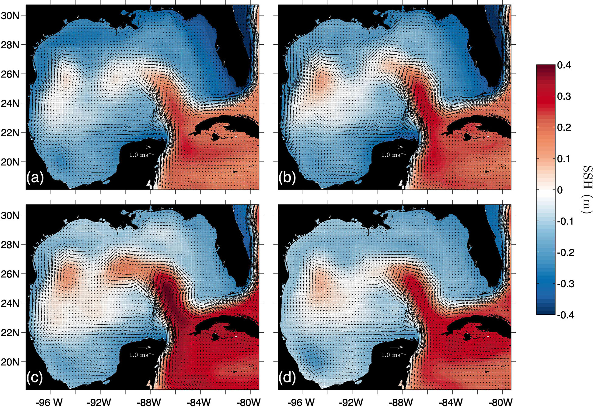
Figure 7 Seasonal climatologies of sea surface height (SSH) and surface circulation for winter (A), spring (B), summer (C) and autumn (D).

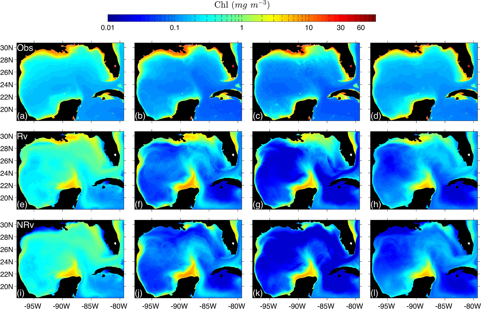
Figure 8 Observed (top row) and simulated (middle and bottom) seasonal climatologies of surface chlorophyll concentration for winter (A, E, I), spring (B, F, J), summer (C, G, K) and autumn (D, H, L). Obs, Observed; Rv, Model configuration with rivers implemented; NRv, Model configuration with no rivers.

Regarding the biogeochemical component of the model, it was possible to acceptably reproduce the general processes involved in the dynamics of chlorophyll as a measure of primary production in the GoM:

• An annual cycle driven by the wind.

• High chlorophyll concentrations in the coastal regions and in cyclonic eddies (primarily in the eddy of the BOC region).

• Low chlorophyll concentrations in the Loop Current and anticyclonic eddies.

4.1 Surface chlorophyll concentration

First we show the simulated surface chlorophyll concentration from both configurations (Rv and NRv) and compare them with satellite images in order to illustrate typical interannual and seasonal patterns. For the 21 years of simulation, in region I and II we observed relatively strong correlations with r=0.60 for both regions, between the monthly averages of the model and those obtained from satellite images (Figure 4). In contrast, a relatively low correlation was observed in region III for these variables (Figure 4). The simulated concentrations were similar to those reported by Xue et al. (2013); Damien et al. (2018); Gomez et al. (2018). The values obtained from the simulations are consistent with those from previous studies on physical-biogeochemical models (i.e., Fennel et al. (2011); Xue et al. (2013); Damien et al. (2018); Gomez et al. (2018)) and with the observational data of Hidalgo-González and Alvarez-Borrego (2008) and Pasqueron de Fommervault et al. (2017). We observed average values of 0.02–0.5 mg m⁻³ in the deep region (Figure 4I) along with a high concentration of chlorophyll (> 5 mg m⁻³) in the Mississippi River delta, which the model was able to mostly reproduce for the spring months (Figure 8F).

Regarding the annual cycle of chlorophyll concentration in the surface, it appears to be stable and consistent with the model data that has been reported by Fennel et al. (2011); Xue et al. (2013); Damien et al. (2018); Gomez et al. (2018), cruise data analyzed by Hidalgo-González and Alvarez-Borrego (2008), and profiler data analyzed by Pasqueron de Fommervault et al. (2017) for both the surface and water column. In the model, this cycle responds mainly to intense vertical mixing caused by winds associated with cold fronts that occur during October–March, mesoscale processes that are mainly associated with the Loop Current, and the eddies that emerge from the Loop Current and eject filaments of chlorophyll-rich water to the central region of the gulf as demonstrated by Toner et al. (2003).

In winter, the model simulated the response of chlorophyll to the supply of nutrients that reach the euphotic zone exported from the upper portion of the nutrient layer due to intense vertical mixing related to atmospheric forcing (e.g., cold fronts from the pole entering the gulf) as shown in panels of Figure 8A, E, I. Such response was evident in the deep region for the satellite images and both model configurations. Nevertheless, it was not the case for the continental shelf where important differences in the chlorophyll concentration can be observed between the Rv and NRv configurations (Figures 8E, I). The most evident was the LATEX region, where the Mississippi and Atchafalaya rivers contribute with the greatest amount of nutrients reaching the continental shelf, dominating the response of the chlorophyll concentration.

In spring it is possible to highlight two processes: a decrease in the surface chlorophyll concentration over the deep region associated with a reduction in wind intensity and increase in chlorophyll concentration over the different regions of the continental shelf (i.e., LATEX, TAVE, and BOC) (Figures 8B, F, J). The increase in chlorophyll over these regions was mainly associated with two factors: the change in the direction of the upwelling-favorable wind component, which can be observed in the response of chlorophyll to the magnitude and direction of the wind patterns in TAVE and BOC (Figures 5A–D), and an accumulation of terrestrial nutrients transported by rivers (Figures 5E, F), which was primarily observed over the LATEX platform in the observations (Figure 8B) and the Rv configuration (Figure 8F). In this region, nutrient inputs, which are mostly supplied by the Mississippi and Atchafalaya rivers, occur during late winter and early spring (Walsh et al., 1989; Turner and Rabalais, 1999). This process continues during the summer, and a minimum concentration of chlorophyll is observed at the surface due to water-column stratification in the deep region.

In contrast, it is during the summer where the greatest difference between model configurations (Rv and NRv) could be observed on the Mexican shelf (Figures 8G, K), principally over the BOC region. This difference was associated with the volume that entered through the Grijalva and Usumacinta rivers, which presented the highest flows in the southern region of the gulf. The average flow of the GrijalvaUsumacinta system was ∼ 3600 m³ s ⁻¹ with maximum values up to 10000 m³ s ⁻¹, suggesting that the nitrate contribution of the Grijalva-Usumacinta system has a fundamental role in the chlorophyll response as demonstrated by the EOF and coherence analysis. Nevertheless, as we described below, the EOF and coherence analysis also showed that the prevailing upwelling-favorable trade winds have an important effect on the surface chlorophyll concentration most of the year, intensifying this effect during the summer

During autumn, the chlorophyll concentration in the deep region gradually increases until the aforementioned winter conditions are once again observed. During the same period, we observed the minimum surface chlorophyll concentration in the Mexican shelf (Figures 8H, L).

Additionally, in the TAVE region it was possible to observe the annual cycle of chlorophyll response in both model configurations, in which low concentrations were present in the coastal zone during the cold months (October–March) and higher concentrations were present during warm months (April–September). However, compared to BOC, the chlorophyll concentration in the TAVE region showed a response associated mainly with the N-S component of the prevailing winds, with higher surface chlorophyll concentrations during the summer when the N-S wind component is upwelling-favorable. In this region, the rivers have a minor impact on the chlorophyll dynamics since the nitrate that flows into the gulf through these is much less than in the BOC and LATEX regions (Figures 5E, F), with mean values of 1.8758 ×10⁷ mol N yr⁻¹, which contrasts with the mean of 1.445 ×10⁸ mol N yr⁻¹ for BOC and what Fennel et al. (2011) reported for the LATEX region: 4.5-5.7 × 10¹⁰ mol N yr⁻¹ for the 1990-2004 period.

The most significant difference between the observed and simulated surface chlorophyll occurred in the LATEX region and in the northern zone of the Yucatan shelf with differences ranging from ∼3 mg m⁻³ to ∼5 mg m⁻³ in LATEX and from ∼1 mg m⁻³ to ∼3 mg m^-3 in the Yucatan shelf, for the Observed and Rv climatologies (Figures 8A–H). Such a difference could be related to the fact that in coastal areas the optical properties of the water are influenced by other constituents of continental origin, such as colored dissolved organic matter (CDOM) and other particles (O’Reilly et al., 1998; Gregg and Casey, 2004). This is important because the algorithms used to measure surface chlorophyll concentration using satellite images were developed for oceanic waters where the optical properties depend only on the chlorophyll concentration of the phytoplankton (Morel and Maritorena, 2001). The chlorophyll concentration discrepancy in the Yucatan shelf could be the product of the high nitrate concentration in the databases used to force the model and to the temperature driven productivity curve proposed by Eppley (1972) used by this model. Other factors that could be influencing this difference are: the morphological characteristics of the Yucatan shelf and the prevailing easterly wind, which is upwelling favorable throughout the year.

4.2 Vertical chlorophyll distribution

The model was able to coherently reproduce the chlorophyll concentration, depth, and migration period of the subsurface maximum at the analyzed point in the water column. We compare values and depths of the simulated chlorophyll in the water column sampled in point P1 (Figure 1) for the 21 years of simulation of the Rv configuration with the reported by Pasqueron de Fommervault et al. (2017) and Damien et al. (2018) and were found to be consistent, reflecting the stable behavior of the primary production processes at work in this region of the gulf. In our simulations, we were able to identify three major processes, which we describe below. First, in winter a uniform vertical distribution of chlorophyll was observed from the surface to the depth of the mixed layer, which was defined as the depth at which the difference in density with regard to the reference depth (in this case 10 m) was 0.03 kg m⁻³. Second, in summer the subsurface maximum was located between 40–90 m on average, and a maximum concentration of ∼ 0.5 mg m⁻³ was observed (Figure 9). Both results are consistent with the data of Pasqueron de Fommervault et al. (2017) derived from APEX profilers, and data simulated by Damien et al. (2018) using a physical-biogeochemical model configuration that was different to the one used in the present study. Then, in the vertical profile of the chlorophyll concentration, it was possible to locate qualitatively the passage of anticyclonic eddies released from the Loop Current which can be observed as periods in which there is no significant concentration of chlorophyll in the water column as shown in Figure 9. The most evident were those that occurred during 1995–1999, 2000–2002, 2004–2008, 2010, and 2013.

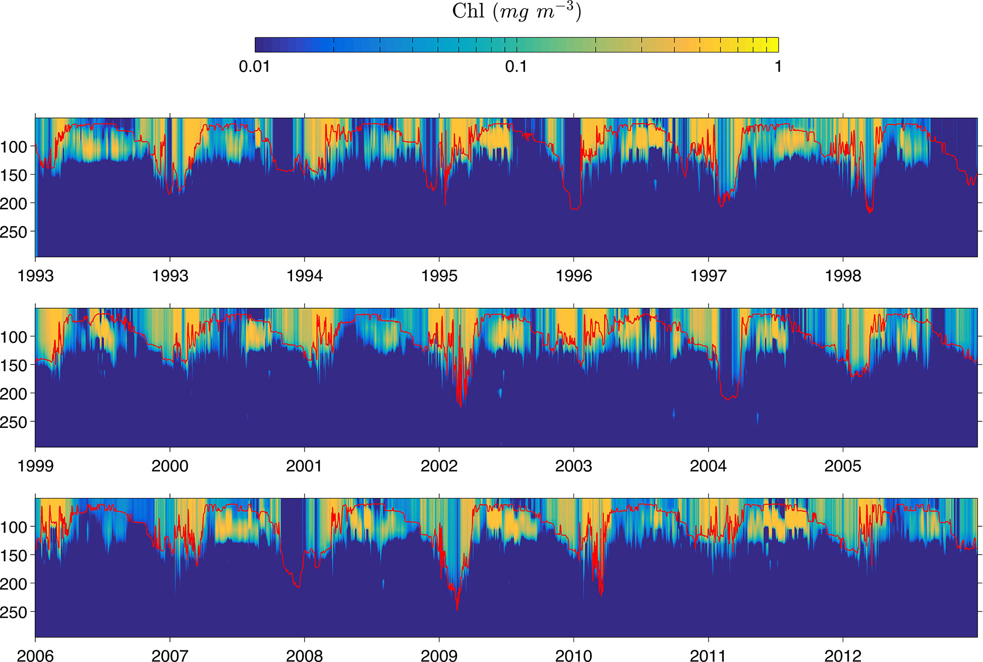
Figure 9 Daily chlorophyll concentration from surface to 250 m sampled in P1. The mixed layer depth (MLD) is represented by the red line.

4.3 Coherence

Regarding the coherence between the mean surface chlorophyll concentration of the Rv configuration and upwelling favorable wind component ${\gamma }^2(Chla-wind)$. We found that the annual signal dominated in both the BOC and TAVE regions with values of ${\gamma }^2{(Chla-wind)}_{BOC}$ =0.90 (Figure 6A) and ${\gamma }^2{(Chla-wind)}_{TAVE}$ =0.95 (Figure 6B). A second important peak of ${\gamma }^2{(Chla-wind)}_{BOC}$ =0.85 and ${\gamma }^2{(Chla-wind)}_{TAVE}$ =0.85 was observed in the 180 day and 60 day period, in both the BOC and TAVE regions, respectively (Figures 6A, B). The dominance of the annual wind cycle in the dynamics of the analyzed regions was identified from the coherence calculation. Such a cycle, in TAVE is associated with the annual upwelling-favorable southerly winds during summer (Figure 5B) and in BOC with the dominant easterly direction of the trade winds (Figure 5A). This contrasts with what was observed in the deep region (Figures 8A, E, I), in which the annual cycle of the response of surface chlorophyll was associated with intense vertical mixing mainly due to cold fronts in the winter months as previously established in several studies (Jolliff et al., 2008; Salmerón-García et al., 2011; Muller-Karger et al., 2015). We associated the 180 day correlation peak observed in TAVE with extraordinary southerly winds during the cold months (October–March). Such winds stimulate a response in the concentration of surface chlorophyll by favoring upwelling due to Ekman transport.

With the purpose of emphasizing the influence of rivers in the TAVE and BOC shelves and considering the fact that the only difference between the Rv and NRv configurations is the river forcing. We propose that, the difference of surface chlorophyll concentration between the two model configurations ($\text{Δ}Chl$) contains the full effect of rivers. Therefore, we present the coherence results (Figures 6C, D) between the nitrate flux ($N{O}_{3}flux$) reaching each region and the corresponding surface chlorophyll difference between the Rv and NRv configurations ($\text{Δ}Chl$). In the same way that the $Chla-wind$ coherence, the $\text{Δ}Chl-N{O}_{3}flux$ coherence [${\gamma }^2(\text{Δ}Chl-N{O}_{3}flux)$] is dominated by an annual signal which is linked to the hydrological cycle of rivers. This effect is more evident in the BOC region with a ${\gamma }^2{(\text{Δ}Chl-N{O}_{3}flux)}_{BOC}$ =0.83 (Figure 6C) compared to the ${\gamma }^2{(\text{Δ}Chl-N{O}_{3}flux)}_{TAVE}$ =0.67 (Figure 6D) present in the TAVE region. Furthermore, in the BOC region the lower frequencies showed higher coherence values, ${\gamma }^2{(\text{Δ}Chl-N{O}_{3}flux)}_{BOC}$ =0.85 for the 66 day period and ${\gamma }^2{(\Delta Chl-N{O}_{3}flux)}_{BOC}$ =0.90 for the 50 day period (Figure 6C). This suggest that the peak of the 60 day period with ${\gamma }^2{(Chla-wind)}_{BOC}$ =0.83 (Figure 6A) is associated to the river effect and not the wind, since the complete Rv signal was used to calculate this value. Conversely, it is not the case for the TAVE region where lower frequency coherence loses relevance, suggesting that the wind effect dominates the chlorophyll response and the effect of the rivers only becomes relevant in the annual period.

4.4 Empirical orthogonal funcions

We examine the EOF for the TAVE region (Figure 10); the first mode yielded 51% and 73% of the variance for the observed and simulated data, respectively. This mode is mainly associated with two factors: the effect of rivers (local and remote) and variations in the chlorophyll concentration associated with atmospheric events. The latter is related to multiple processes such as cold fronts (which induce vertical mixing) and extraordinary winds from the south (upwelling favorable winds).

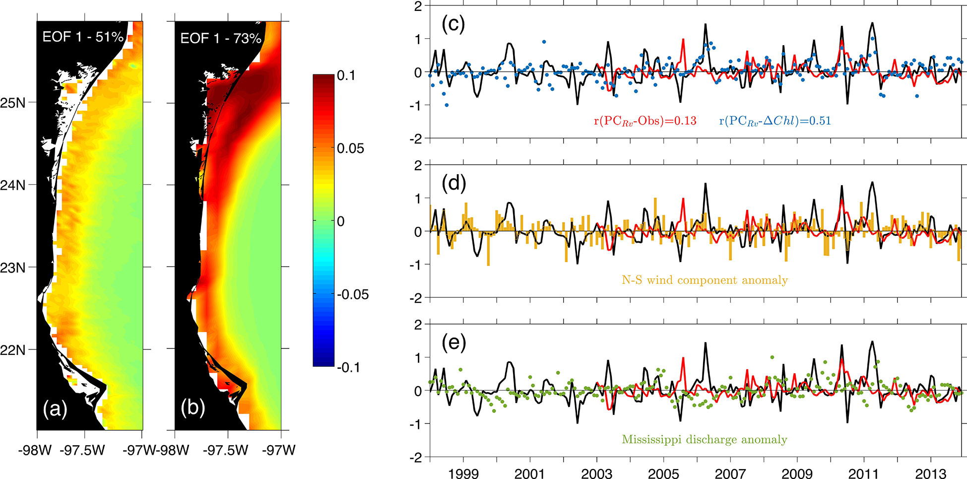
Figure 10 First mode of the surface chlorophyll EOF calculated in the Tamaulipas-Veracruz (TAVE) region. Panel (A) - Spatial structure from monthly satellite imagery products. Panel (B) - Spatial structure from the model outputs. Panel (C) - Principal component corresponding to mode 1 for the model outputs (black line) and observed data (red line), the blue dots represent the surface chlorophyll difference ($\Delta Chla$) between model configurations (i.e. Rv and NRv) for the TAVE region. Panel (D) - Monthly averaged N-S wind component anomaly in the TAVE shelf. Panel (E) - Discharge anomaly from the Mississippi River.

In TAVE, the peaks in extraordinary variability observed in the years 1998, 1999 and 2000, are associated with the strong upwelling-favorable wind (Figure 10D) and the associated Mississippi and Atchafalaya waters advected from LATEX to TAVE. The latter, since it is known that water from these rivers is advected onto TAVE during autumn and winter months Zavala-Hidalgo et al. (2003). This was particularly noticeable in the years 1998 and 1999 (Figure 10E). Moreover, the variability peaks associated with extraordinary flow from the local rivers can be observed in 2004, 2006 and the period between 2009 and 2011 (Figure 10C) appears to be happening only in the model PC, except for 2010 where a response in the observed PC is also present. It is important to note that in the years 2006 and 2011 an increase in the intensity of favorable winds for upwelling was also observed (Figure 10D), which could have led to greater variability in the response of chlorophyll.

For the BOC region (Figure 11), a response to the annual flow cycle of the relevant rivers of the Grijalva-Usumacinta system in the region was observed with a correlation coefficient of 0.60 between the PC of the first mode and the monthly averaged $\text{Δ}Chla$ (Figure 11C). Such response of surface chlorophyll due to the effect of rivers represented the 54% and 66% of the variance for the observed and simulated data, respectively. Since the intensity and variability of the wind is small in this area (Figure 11D), most of the years that present relevant variability peaks in the PC (e.g. 1998-2001, 2005, 2007, 2008, 2010 and 2011) are related to the contribution of nutrients associated with extraordinary flow events from the rivers, mainly the Grijalva-Usumacinta system which has the highest discharge rates compared to other rivers in the region.

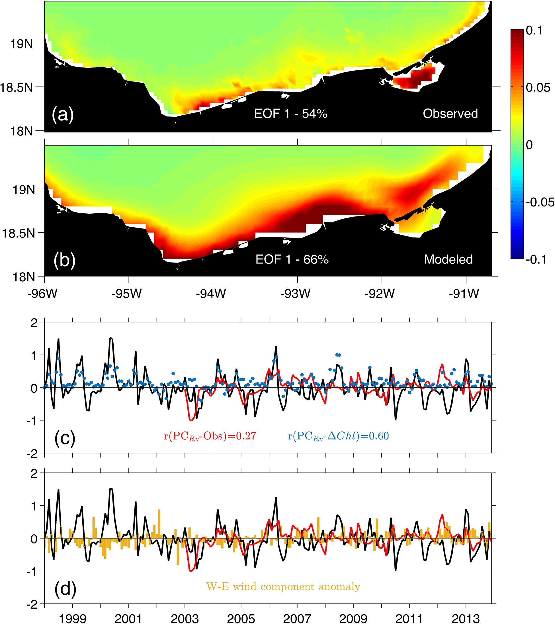
Figure 11 First mode of the surface chlorophyll EOF calculated in the Bay of Campeche (BOC) region. (A) spatial structure from monthly satellite imagery products. (B) spatial structure from the model outputs. (C) Principal component corresponding to mode 1 for the model outputs (black line) and observed data (red line), the blue dots represent the surface chlorophyll difference ($\Delta Chla$) between model configurations (i.e. Rv and NRv) for the BOC region. (D) Monthly averaged W-E wind component anomaly in the BOC shelf.

5 Conclusions

On the whole, we can conclude that using realistic discharge and nutrient data in river forcing improves the way in which primary production processes in coastal areas are represented by coupled physical-biogeochemical models. Moreover, by using this data, in some cases we were able to observe a response in chlorophyll concentration to extraordinary events related to hydrological and anthropogenic processes.

We found that in the deep region of the gulf, the concentration and distribution (both superficial and in the water column) of chlorophyll was mainly driven by the annual wind cycle, which was associated with the formation of cold fronts. In BOC, the variation in the chlorophyll concentration was driven by two main factors. The first was the nitrate concentration, provided mainly by the Grijalva-Usumacinta river system, which is directly correlated to the hydrological annual cycle but also to lower frequency events that could be related to variations in nitrate concentration associated to anthropogenic activities. The second was the prevailing wind in the region which is upwelling-favorable throughout the year. In TAVE, three determining factors were found for the chlorophyll response. The main factor was the annual wind cycle which is driven by the N-S wind component and it is upwelling-favorable in the summer and downwelling-favorable in winter. The second factor was the nutrients provided by local rivers which, in specific years, provided sufficient nitrate to trigger a chlorophyll response. The third factor was the contribution from the Mississippi and Atchafalaya rivers, which advect their waters into the TAVE shelf in the autumn and winter months.

Altogether, due to the fact that there is no continuous data of in situ chlorophyll concentration in the studied regions and to the limitations that satellite products have to measure this variable in coastal areas, the use of physical-biogeochemical models is fundamental to study and describe the mechanics of the biological response to the continental and oceanic contribution of nutrients.

Data availability statement

The raw data supporting the conclusions of this article will be made available by the authors, without undue reservation.

Author contributions

Conceptualization: JG-R, AP-S; Data curation: JG-R, AP-S, JC-M; Formal analysis: JG-R, AP-S; Funding acquisition: AP-S; Investigation: JG-R; Methodology: JG-R, AP-S; Project administration: AP-S; Resources: AP-S; Software: JG-R, AP-S; Supervision: AP-S; Validation: JG-R, AP-S; Visualization: JG-R; Writing – original draft: JG-R; Writing – review & editing: JG-R, AP-S, JC-M. All authors contributed to the article and approved the submitted version.

Funding

This research has been funded by the Mexican National Council for Science and Technology (CONACYT) and the Mexican Ministry of Energy Trust, projects CF-MG-20191030200716411-1727972 and 201441.

Acknowledgments

This is a contribution of the Gulf of Mexico Research Consortium (CIGoM). We acknowledge PEMEX specific request to the Hydrocarbon Fund to further the knowledge on the environmental effects of oil spills in the Gulf of Mexico. This study was conducted using E.U. Copernicus Marine Service Information.

Conflict of interest

The authors declare that the research was conducted in the absence of any commercial or financial relationships that could be construed as a potential conflict of interest.

Publisher’s note

All claims expressed in this article are solely those of the authors and do not necessarily represent those of their affiliated organizations, or those of the publisher, the editors and the reviewers. Any product that may be evaluated in this article, or claim that may be made by its manufacturer, is not guaranteed or endorsed by the publisher.

References

Biltoft C. A., Pardyjak E. R. (2009). Spectral coherence and the statistical significance of turbulent flux computations. J. atmospheric oceanic Technol. 26, 403–409. doi: 10.1175/2008JTECHA1141.1
Boyer T. P., Antonov J. I., Baranova O. K., Coleman C., Garcia H. E., Grodsky A., et al. (2013). World ocean database 2013 (NOAA). https://repository.library.noaa.gov/view/noaa/1291
CONAGUA (2014). “Estadísticas del agua en méxico,” in Gerencia de aguas superficiales e ingeniería de ríos (Commisón Nacional del Agua). https://www.conagua.gob.mx/conagua07/publicaciones/publicaciones/eam2014.pdf
Damien P., Pasqueron de Fommervault O., Sheinbaum J., Jouanno J., Camacho-Ibar V. F., Duteil O. (2018). Partitioning of the open waters of the gulf of mexico based on the seasonal and interannual variability of chlorophyll concentration. J. Geophysical Research: Oceans 123, 2592–2614. doi: 10.1002/2017JC013456
Debreu L., Marchesiello P., Penven P., Cambon G. (2012). Two-way nesting in split-explicit ocean models: algorithms, implementation and validation. Ocean Model. 49, 1–21. doi: 10.1016/j.ocemod.2012.03.003
Elliott B. A. (1982). Anticyclonic rings in the gulf of mexico. J. Phys. Oceanography 12, 1292–1309. doi: 10.1175/1520-0485(1982)012<1292:ARITGO>2.0.CO;2
Fennel K., Hetland R., Feng Y., Dimarco S. (2011). A coupled physical-biological model of the northern gulf of Mexico shelf: Model description, validation and analysis of phytoplankton variability. Biogeosciences 8, 1881–1899. doi: 10.5194/bg-8-1881-2011
Fennel K., Wilkin J., Levin J., Moisan J., O’Reilly J., Haidvogel D. (2006). Nitrogen cycling in the middle atlantic bight: Results from a three-dimensional model and implications for the north atlantic nitrogen budget. Global Biogeochemical Cycles 20. doi: 10.1029/2005GB002456
Gomez F. A., Lee S.-K., Liu Y., Hernandez J. F.J., Muller-Karger F. E., Lamkin J. T. (2018). Seasonal patterns in phytoplankton biomass across the northern and deep gulf of mexico: a numerical model study. Biogeosciences 15, 3567. doi: 10.5194/bg-15-3561-2018
González-Ramírez J., Parés-Sierra A. (2019). Streamflow modeling of five major rivers that flow into the gulf of mexico using swat. Atmósfera 32, 261–272. doi: 10.20937/ATM.2019.32.04.01
Gregg W. W., Casey N. W. (2004). Global and regional evaluation of the seawifs chlorophyll data set. Remote Sens. Environ. 93, 463–479. doi: 10.1016/j.rse.2003.12.012
Gruber N., Frenzel H., Doney S. C., Marchesiello P., McWilliams J. C., Moisan J. R., et al. (2006). “Eddy-resolving simulation of plankton ecosystem dynamics in the california current system,” in Deep Sea research part I: Oceanographic research papers (Elsevier), vol. 53. , 1483–1516. doi: 10.1016/j.dsr.2006.06.005
Hidalgo-González R., Alvarez-Borrego S. (2008). Water column structure and phytoplankton biomass profiles in the gulf of mexico. Cienc. Marinas 34, 197–212.
Jolliff J. K., Kindle J. C., Penta B., Helber R., Lee Z., Shulman I., et al. (2008). On the relationship between satellite-estimated bio-optical and thermal properties in the gulf of mexico. J. Geophysical Research: Biogeosciences 113. doi: 10.1029/2006JG000373
Large W. G., McWilliams J. C., Doney S. C. (1994). Oceanic vertical mixing: A review and a model with a nonlocal boundary layer parameterization. Rev. Geophysics 32, 363–403. doi: 10.1029/94RG01872
Lellouche J.-M., Le Galloudec O., Greiner E., Garric G., Regnier C., Drevillon M., et al. (2013). The copernicus marine environment monitoring service global ocean 1/12 physical reanalysis glorys12v1: description and quality assessment. EGU General Assembly Conference Abstracts 20, 19806.
Lohrenz S. E., Fahnenstiel G. L., Redalje D. G., Lang G. A., Chen X., Dagg M. J. (1997). Variations in primary production of northern gulf of mexico continental shelf waters linked to nutrient inputs from the mississippi river (Inter-Research), Vol. 155, 45–54. doi: 10.3354/meps15504
Morel A., Maritorena S. (2001). Bio-optical properties of oceanic waters: A reappraisal. J. Geophys. Res.: Oceans 106, 7163–7180. doi: 10.1029/2000JC000319
Muller-Karger F. E., Smith J. P., Werner S., Chen R., Roffer M., Liu Y., et al. (2015). Natural variability of surface oceanographic conditions in the offshore gulf of mexico. Prog. Oceanogr. 134, 54–76. doi: 10.1016/j.pocean.2014.12.007
Nababan B., Muller-Karger F. E., Hu C., Biggs D. C. (2011). Chlorophyll variability in the northeastern gulf of mexico. Int. J. Remote Sens. 32, 8373–8391. doi: 10.1080/01431161.2010.542192
O’Reilly J. E., Maritorena S., Mitchell B. G., Siegel D. A., Carder K. L., Garver S. A., et al. (1998). Ocean color chlorophyll algorithms for seawifs. J. Geophysical Research: Oceans 103, 24937–24953. doi: 10.1029/98JC02160
Pasqueron de Fommervault O., Perez-Brunius P., Damien P., Camacho-Ibar V. F., Sheinbaum J. (2017). Temporal variability of chlorophyll distribution in the gulf of mexico: bio-optical data from profiling floats. Biogeosciences 14, 5647–5662. doi: 10.5194/bg-14-5647-2017
Saha S., Moorthi S., Pan H.-L., Wu X., Wang J., Nadiga S., et al. (2010). “The ncep climate forecast system reanalysis,” in Bulletin of the American Meteorological Society (American Meteorological Society), Vol. 91. 1015–1058. doi: 10.1175/2010BAMS3001.1
Saha S., Moorthi S., Wu X., Wang J., Nadiga S., Tripp P., et al. (2014). Ncep climate forecast system version 2. J. Clim. 27 (6), 2185–2208. doi: 10.1175/JCLI-D-12-00823.1
Salmerón-García O., Zavala-Hidalgo J., Mateos-Jasso A., Romero-Centeno R. (2011). Regionalization of the gulf of mexico from space-time chlorophyll-a concentration variability. Ocean Dynamics 61, 439–448. doi: 10.1007/s10236-010-0368-1
Toner M., Kirwan A. Jr., Poje A., Kantha L., Müller-Karger F., Jones C. (2003). Chlorophyll dispersal by eddy-eddy interactions in the gulf of mexico. J. Geophys. Res.: Oceans 108. doi: 10.1029/2002JC001499
Turner R., Rabalais N. (1999). Suspended particulate and dissolved nutrient loadings to gulf of mexico estuaries. Biogeochemistry Gulf Mexico Estuaries, 89–107.
Vázquez De La Cerda A. M., Reid R. O., DiMarco S. F., Jochens A. E. (2005). Bay of campeche circulation: An update. Circ. Gulf Mex. Obs. Model. 161, 279–293. doi: 10.1029/161GM20
Walsh J. J., Dieterle D. A., Meyers M. B., Müller-Karger F. E. (1989). Nitrogen exchange at the continental margin: A numerical study of the gulf of mexico. Prog. Oceanography 23, 245–301. doi: 10.1016/0079-6611(89)90002-5
Wang S., Tang M. (2004). Exact confidence interval for magnitude-squared coherence estimates. IEEE Signal Process. Lett. 11, 326–329. doi: 10.1109/LSP.2003.822897
Woodruff S. D., Slutz R. J., Jenne R. L., Steurer P. M. (1987). A comprehensive ocean-atmosphere data set. Bulletin of the American meteorological society 68 (10), 1239–1250. doi: 10.1175/1520-0477(1987)068<1239:ACOADS>2.0.CO;2.
Xue Z., He R., Fennel K., Cai W.-J., Lohrenz S., Hopkinson C. (2013). Modeling ocean circulation and biogeochemical variability in the gulf of mexico. Biogeosciences 10, 7219–7234. doi: 10.5194/bg-10-7219-2013
Zavala-Hidalgo J., Gallegos-García A., Martínez-López B., Morey S. L., O’Brien J. J. (2006). Seasonal upwelling on the Western and southern shelves of the gulf of Mexico. Ocean Dyn 56, 333–338. doi: 10.1007/s10236-006-0072-3
Keywords: Gulf of Mexico, biogeochemical processes, chlorophyll, river, discharge
Citation: González-Ramírez J, Parés-Sierra A and Cepeda-Morales J (2023) Chlorophyll response to wind and terrestrial nitrate in the western and southern continental shelves of the Gulf of Mexico. Front. Mar. Sci. 10:1034638. doi: 10.3389/fmars.2023.1034638
Received: 01 September 2022; Accepted: 07 March 2023;
Published: 23 March 2023.
Edited by:
Maria Josefina Olascoaga, University of Miami, United StatesReviewed by:
James Acker, National Aeronautics and Space Administration (NASA), United StatesGabor Varbiro, Hungarian Academy of Sciences, Hungary
Copyright © 2023 González-Ramírez, Parés-Sierra and Cepeda-Morales. This is an open-access article distributed under the terms of the Creative Commons Attribution License (CC BY). The use, distribution or reproduction in other forums is permitted, provided the original author(s) and the copyright owner(s) are credited and that the original publication in this journal is cited, in accordance with accepted academic practice. No use, distribution or reproduction is permitted which does not comply with these terms.
*Correspondence: Alejandro Parés-Sierra, apares@cicese.mx