Late Pleistocene to Holocene variations in marine productivity and terrestrial material delivery to the western South Atlantic

Introduction

Temporal changes in carbon source delivery have been frequently recorded in ocean sediments. They can explain the linkages among climate, organic matter (OM) biogeochemical cycling, and carbon sequestration over different time scales (Faux et al., 2011). The South Atlantic Ocean plays an essential role in the global climate system by forming nutrient-rich dense water masses and promoting heat transport into the Southern Ocean (Garzoli and Matano, 2011). It also receives large amounts of terrestrial OM originating from South America [e.g., Rio de la Plata (RdlP) Basin] and Africa (e.g., Congo basin) (Weijers et al., 2007; Muelbert et al., 2008). The delivery of terrestrial OM to the ocean can function as a long-term sink and, consequently, a significant CO₂ sequestration mechanism (Sarmiento and Gruber, 2006). Along with the terrestrial OM input, rivers also deliver nutrients to the adjacent ocean, promoting marine productivity (Bianchi et al., 2018).

Knowledge about variations in the terrestrial input and primary productivity is crucial for the comprehension of past climate changes in the Southern Hemisphere, especially in the southeastern (SE) part of South America. This knowledge is expected to provide insights into the natural trends of climate variability for the next millennia. Also, the South Atlantic plays a major role in the world ocean overturning circulation. Specifically, the southwest (SW) Atlantic margin is marked by a strong N–S dynamics, characterized by the southward flow of the North Atlantic Deep Water and the northward flow of the Antarctic Intermediate Water, two of the main components of the meridional circulation in the Atlantic Ocean (Mahiques et al., 2022). Several studies have reported temporal variations in OM input to the continental margin of the SW Atlantic (e.g., Costa et al., 2016; Lourenço et al., 2016; Gu et al., 2017) and put forth distinct mechanisms governing marine paleoproductivity and terrestrial OM input. Portilho-Ramos et al. (2015) and Pereira et al. (2018) related high rates of marine paleoproductivity in the SW Atlantic to upwelling of the South Atlantic Central Water (SACW) promoted by the Brazil Current (BC) eddies. Other studies associated elevated marine productivity in the South Brazil Bight (SBB) with periods of greater terrestrial inputs (Mahiques et al., 2007; Nagai et al., 2010; Lourenço et al., 2016; Gu et al., 2017). Therefore, the primary mechanism controlling marine productivity in the SBB central portion remains unresolved.

Terrestrial OM content in continental margin sediments may vary in response to the type and amount of OM produced on the continent and exported to the ocean. An additional factor is the distance of the core site to the continent, which is a function of sea level that affects the continental shelf width. Previous studies in the region (Mahiques et al., 2007; Nagai et al., 2010; Lourenço et al., 2016) focused on terrestrial OM amount but did not investigate the sources. Presently, the RdlP drains the inner portion of the southern part of South America and influences only the southern portion of the SBB (Nagai et al., 2014a; Razik et al., 2015), whereas the northern portion receives sediments carried by the southward BC (Nagai et al., 2014a). A recent study (Mahiques et al., 2017) on core top sediments (including NAP 63-1) from the continental shelf and slope in the central portion of SBB suggested that terrestrial input to the mid-slope is influenced by the northward Intermediate Western Boundary Current (IWBC) rather than by the southward BC (Figure 1).

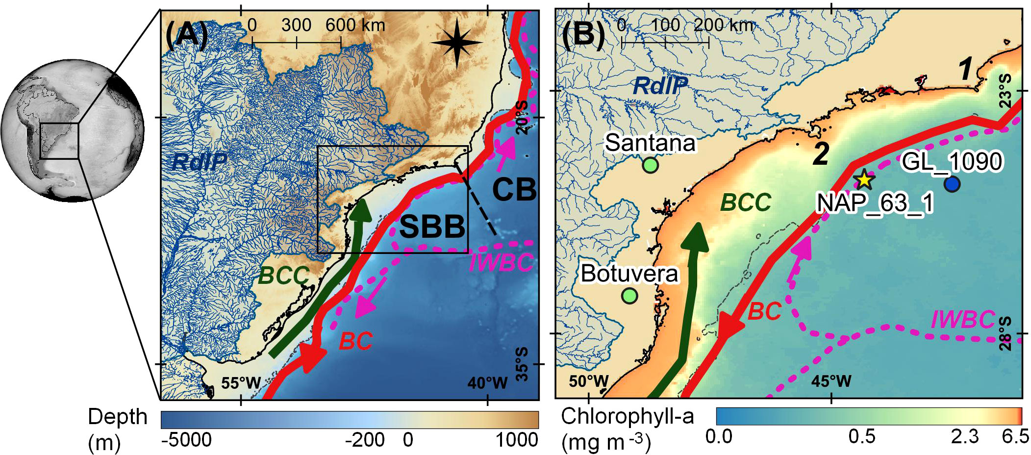
Figure 1 (A) Indication of the main ocean currents in the SW Atlantic as well as the location of Campos Basin (CB) and South Brazil Bight (SBB) separated by the black dashed line. The black rectangle is displayed in map B. (B) Map highlighting the SBB with the location of sediment core NAP 63-1 (yellow star), GL-1090 (blue circle), and the speleothem sites (green circles) used in the discussion. The gray dashed line indicates the continental shelf break. Current names, BC, Brazil Current; BCC, Brazil Coastal Current; IWBC, Intermediate Western Boundary Current. Geographical features: 1 - Cabo Frio; 2 - São Sebastião Island.

In this study, we quantified markers in SBB mid-slope sediments [n-alkanes, long-chain alkenones (LCA), glycerol dialkyl glycerol tetraethers (GDGTs), n-alkanols, sterols, and long-chain diols] to evaluate the sources of OM delivered to the site, and how these sources varied over time, from the Late Pleistocene to the Holocene. We investigated the primary mechanism controlling marine productivity in the SBB central portion as well as the main delivery routes of the terrestrial OM to the region. Molecular organic biomarkers can provide insights into OM sources to aquatic environments and OM sequestration to sediments over decadal to geological time scales. Therefore, they help resolve the complexity in systems with multiple organic carbon sources (Yunker et al., 2005; Holland et al., 2013). Based on their temporal evolution, we associated the OM flux with oceanographic and climatological processes during the Late Pleistocene and Holocene. We compared the evolution of these organic biomarker contents with other studies from the vicinity of the study site to identify the mechanisms that governed marine productivity and possible sources of terrestrial OM during the Last Glacial Period.

Study area

Today, circulation in the SBB (latitudes 22°S–34°S) is characterized by two western boundary currents, the BC and the IWBC (Figure 1). The BC flows southward and meanders around the 200-m isobath (Campos et al., 2000). It transports warm and oligotrophic tropical water (T > 20°C and S > 36.4) in the first 100 m of the water column, and cold and nutrient-rich SACW (T = 6°C–20°C and S = 34.5–36.4) below 100 m and down to approximately 600-m depth (Silveira et al., 2015). Below the BC, the IWBC flows northward in the SBB, carrying Antarctic Intermediate Water (T = 3°C–7°C and S = 24.6–34.4) down to approximately 1,100-m depth (Silveira et al., 2015).

The change in the coastline orientation at Cabo Frio induces a meandering pattern in the BC, which frequently becomes unstable, forming strong cyclonic and anticyclonic frontal eddies (Campos et al., 2000). These eddies represent an efficient mechanism for increasing vertical speeds, acting decisively in the upwelling of SACW. This type of meander-induced upwelling brings SACW to shallower depths and fertilizes the otherwise typically oligotrophic waters (Campos et al., 2000; Ribeiro et al., 2016).

The SBB can also be considered a convergence zone regarding OM transport, receiving material from the south through the advancement of the RdlP plume and from the north through the upwelling region of SACW (Mahiques et al., 2004). The area off São Sebastião Island (24°00′S; 45°30′W) marks a regional boundary between the two sedimentary provinces. The RdlP drains the second largest drainage basin in South America and discharges approximately 710 km³ yr⁻¹ (or 22,514 m³ s⁻¹) of freshwater at the RdlP estuary at ~35°S (Razik et al., 2015). This material is redistributed northward up to 27°S by the Brazil Coastal Current (Nagai et al., 2014a), south of the coring site. Aside from the RdlP, the SBB region receives only small contributions of terrestrial material from the adjacent coast, especially from SE Brazil, resulting in little terrestrial input to the coring site.

The adjacent continent is characterized by a narrow (>80 km) coastal lowland (<100-m altitude), limited by the “Serra do Mar” coastal mountain range extending approximately parallel to the coast (Almeida and Carneiro, 1998). The Atlantic rainforest is the typical vegetation of the lowland and the slopes of the “Serra do Mar” mountain range (Ribeiro et al., 2009). The estuaries are mainly dominated by mangrove trees (Rhizophora sp., Avicennia sp., and Languncularia sp.) as far south as 28°30′S, where they are replaced by saltmarshes (formed by Spartina alterniflora) (Schaeffer-Novelli et al., 1990).

Material and methods

Sampling and age model

Sediment core NAP 63-1 was collected on the continental slope of the subtropical southwestern Atlantic (24°50.304′S; 44°19.124′W; 840-m water depth; 2.24-m long) (Figure 1). The distance from the coring site to the coast today is about 140 km. The sampling took place on 26 February 2013, during an RV Alpha Crucis cruise, from the Oceanographic Institute of the University of São Paulo (IO-USP; Brazil), using a piston corer. The core was sectioned every 2 cm, yielding a total of 112 samples. The samples were stored frozen in pre-combusted aluminum trays for further analysis.

The age model for this sediment core was described by Dauner et al. (2019). Briefly, it was based on radiocarbon dating of planktonic foraminifera (AMS ¹⁴C) and benthic foraminifera stable oxygen isotope (δ¹⁸O) tie points aligned to two reference curves (Lisiecki and Raymo, 2005; Lisiecki and Stern, 2016). The downcore ages were modeled using BACON software version 2.3.5 (Blaauw and Christen, 2011). The core material covered approximately the past 78 ka with no observed age inversion in the radiocarbon ages.

Bulk parameters

Analysis of total organic carbon (TOC) content and carbon isotope composition (δ¹³C) was performed on decarbonated dry sediment samples (acid treatment with 1 mol L^–1 HCl solution). Determinations of total nitrogen (TN) content and the nitrogen isotope composition (δ¹⁵N) were performed on dry unacidified sediment. The samples were analyzed by an EA-Costech elemental analyzer coupled to a Thermo Scientific Delta V Advantage isotope ratio mass spectrometer (EA-IRMS). The analytical accuracy was verified using the USGS-40 (L-glutamic acid, United States Geological Survey) and IAEA-600 (caffeine, International Atomic Energy Agency) standards before and after each group of 40 samples. Standard deviations for calibration were within the expected range, being 0.01‰ for both ratios for USGS-40, 0.03‰ for δ¹³C, and 0.09‰ for δ¹⁵N for IAEA-600. The standard used as a reference for carbon and nitrogen contents was Soil LECO (LECO Corporation, USA), whose estimated levels are 13.55% and 0.81% dry weight, respectively, and in agreement with the certified values.

Lipid extraction and purification

About 5 g of freeze-dried and homogenized samples were extracted three times using an ultrasonic bath with 25 ml of methanol:dichloromethane (1:9; v:v). Known amounts of squalene, C₁₉ ketone, 5α-androstanol, and C₄₆ GDGT were added as internal standards before extraction. The combined extracts were evaporated by rotary evaporation under vacuum at 40°C. The total lipid extracts were saponified for 2 h at 80°C with 1 ml of 0.1 mol L⁻¹ KOH in methanol:H₂O (9:1; v:v). After saponification, neutral lipids were liquid–liquid extracted into n-hexane and further purified by passing them over a silica gel column (1% deactivated with water). They were eluted with 4 ml of n-hexane (recovery of n-alkanes), 4 ml of n-hexane:dichloromethane (1:2; v:v; recovery of ketones), and 4 ml of dichloromethane:methanol (1:1; v:v; recovery of n-alkanols, sterols, diols, and GDGTs) and dried using a Silli-Therm at 50°C under a stream of nitrogen.

Before capillary gas chromatography analyses, the n-alkane and alkenone fractions were re-dissolved in 100 μl of n-hexane. The dry polar fractions were weighed and adjusted to concentrations of approximately 2 mg ml⁻¹ by dissolution with isopropanol:n-hexane (1:99; v:v). Before the analysis, the polar fractions were filtered (Thermo Scientific PTFE filter: 4 mm in diameter and 0.45 μm porosity) to retain any remaining particles. These extracts were injected into a high-performance liquid chromatograph coupled to a mass spectrometer. The remaining extracts were then dried and derivatized by adding 30 μl of N,O-bis(trimethylsilyltrifluoroacetamide):trimethylchlorosilane (BSTFA : TMCS; 99:1; v:v) and 30 μl of acetonitrile and heated for 60 min at approximately 60°C. After derivatization, the reagents were dried, and the fraction was re-dissolved in 50 μl of n-hexane before capillary gas chromatography.

Analytical methods

n-Alkanes were analyzed by injecting 2-μl sample aliquots in the split mode in an Agilent 7890A series gas chromatograph equipped with a flame ionization detector and an Agilent DB-5ms capillary fused silica column coated with 5% phenyl/dimethyl arylene siloxane (60-m length, 0.25-mm internal diameter, and 0.25-μm film thickness). Helium was used as the carrier gas with a constant flow rate of 1.5 ml min⁻¹. The initial oven temperature was 60°C, held for 1 min, increased to 150°C at a rate of 20°C min⁻¹, then raised to 320°C at a rate of 6°C min⁻¹ and held for 35 min with a total run time of 69 min. The injector and detector temperatures were adjusted to 250°C and 330°C, respectively.

Alkenones were analyzed by injecting 2-μl sample aliquots in the splitless mode in an Agilent 7890A series gas chromatograph equipped with a flame ionization detector and an Agilent HP-5 capillary fused silica column coated with 5% phenyl/methylpolysiloxane (50-m length, 0.32-mm internal diameter, and 0.17-μm film thickness). Hydrogen was used as the carrier gas with a constant flow rate of 1.2 ml min⁻¹. The initial oven temperature was 40°C, increased to 60°C at a rate of 20°C min⁻¹, then raised to 320°C at a rate of 5°C min⁻¹ and held for 15 min with a total run time of 68 min. The injector and detector temperatures were adjusted to 300°C and 325°C, respectively.

GDGT analyses were performed using an Agilent 1200 Series high-performance liquid chromatography system coupled with an Agilent 6120 mass spectrometer. The 20-μl aliquots were injected into an Alltech Prevail^® Cyano column (2.1 × 150 mm², 3 μm; Grace) maintained at 30°C. GDGTs were eluted using the following gradient with solvent A (n-hexane:isopropanol:chloroform; 98:1:1) and solvent B (n-hexane:isopropanol:chloroform; 89:10:1): 100% A for 5 min, linear gradient to 10% B in 20 min, linear gradient to 100% B in 10 min, and then held for 7 min. The flow rate was 0.2 ml min⁻¹. After each analysis, the column was cleaned by back-flushing with 100% B at 0.6 ml min⁻¹ for 5 min and then held for 10 min in the initial conditions (100% A at 0.2 ml min⁻¹).

n-Alkanols, sterols, and diols were analyzed by injecting 2-μl sample aliquots in the splitless mode in an Agilent 6850A series gas chromatograph equipped with an Agilent 5975C VL MSD mass spectrometer, a Restek Rxi-1ms capillary fused silica column coated with 1% diphenyl/dimethylsiloxane (30-m length, 0.25-mm internal diameter, and 0.25-μm film thickness) and a 5-m precolumn. Helium was used as the carrier gas with a constant flow rate of 1.2 ml min⁻¹. The initial oven temperature was 100°C, held for 8 min, and subsequently increased to 300°C at a rate of 4°C min⁻¹ with a total run time of 58 min. The injector temperature was set to 280°C and operated in splitless injection mode. The detector and ion source temperatures were set to 280°C and 230°C, respectively.

n-Alkanes were individually identified by matching retention times against a standard containing the homologous series from n-C₁₄ to n-C₄₀. LCA were identified by matching retention times against a standard containing C₁₉ ketone and C_37:2 and C_37:3 alkenones. n-Alkanol, sterol, and diol data were acquired using the selected ion monitoring mode, and they were identified by the ion fragments characteristic of each compound (Supplementary Tables S1–S3). GDGT data were also acquired using the selected ion monitoring mode, but they were identified by the molecular ions (Supplementary Table S4).

The following compounds were quantified and will be used in the discussion: (i) n-alkanes: odd-numbered n-C₁₅ to n-C₃₉; (ii) LCA: C_37:3 methyl, C_37:2 methyl, C_38:3 methyl and ethyl, C_38:2 methyl and ethyl, C_39:3 ethyl, and C_39:2 ethyl; (iii) n-alkanols: even-numbered n-C₁₂-OH to n-C₃₄-OH; (iv) phytol; (v) sterols: 27Δ^5,22E (dehydrocholesterol), 27Δ⁵ (cholesterol), 28Δ^5,22E (brassicasterol), 28Δ⁵ (campesterol), 29Δ^5,22E (stigmasterol), 29Δ⁵ (sitosterol), and 30Δ^22E (dinosterol); (vi) long-chain diols: C₂₈1,14 and C₃₀1,14; and (vii) GDGTs: crenarchaeol, branched GDGT-IIIa, branched GDGT-IIa, and branched GDGT-Ia. The quantification was done via internal standards by assuming identical response factors as the respective compounds.

Procedural blanks were analyzed for each set of 15 samples, and they showed no significant level peaks in the analyses of target compounds. Finally, four replicates of the same sediment sample were extracted and used as an internal laboratory reference. The coefficient of variation among the four replicates was lower than 25% for all the compounds.

Data processing

A cluster using SAX (Symbolic Aggregate approXimation) representation (Lin et al., 2007) in the dissimilarity measure calculation was used to group the different proxies according to their evolutions through time. SAX representation is a “structured-based” dissimilarity measure that focuses on comparing underlying dependence structures, being suitable to analyze long time series. The symbolization approach involves transformation of time series into sequences of discretized symbols, allowing dimensionality reduction but keeping the distance measures defined on the original time series (Lin et al., 2007). Thus, the cluster analysis using SAX representation in the dissimilarity measure can be used to group different proxies according to their temporal evolution, regardless of their concentration ranges. For this analysis, we used packages “TSclust” (Montero and Vilar, 2014), “vegan” (Oksanen et al., 2018), and “rioja” (Juggins, 2017) with R environment version 4.1.2 (R Core Team, 2021).

Two groups were formed based on the cluster analysis previously mentioned: the “terrestrial-source” group and the “marine-source” group (Dauner et al., 2020) (Figure 2). For all samples, contents of the organic biomarkers (in ng g⁻¹ dry sediment) were converted to mass accumulation rates (MAR) using the sedimentation rates from Dauner et al. (2019). As the dry bulk density values for NAP 63-1 were not determined, we used mean dry bulk density values obtained by Müller (2004) for a nearby sediment core from the SBB (core GeoB 2107-3; 27.18°S, 46.45°W, 1,048-m water depth).

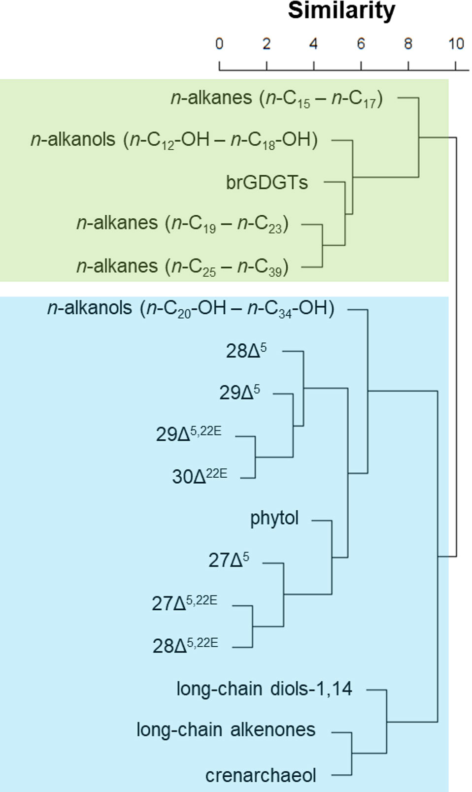
Figure 2 Cluster analysis based on the temporal evolution of each organic compound group, using the SAX representation as the dissimilarity measure. The green rectangle indicates the “terrestrial-source” group and the blue rectangle indicates the “marine-source” group.

After the organic markers were separated into these two groups, a constrained cluster analysis was performed, considering the groups separately to define stratigraphical zones. For this analysis, we used accumulation rates of the following organic compounds: mid-chain odd-numbered n-alkanes (n-C₁₉ – n-C₂₃), long-chain odd-numbered n-alkanes (n-C₂₅ – n-C₃₉), LCA, crenarchaeol, branched GDGTs, short-chain even-numbered n-alkanols (n-C₁₂-OH – n-C₁₈-OH), long-chain even-numbered n-alkanols (n-C₂₀-OH – n-C₃₄-OH), phytol, C₂₈ and C₃₀ 1,14-diols, and the sterols 27Δ^5,22E, 27Δ⁵, 28Δ^5,22E, 28Δ⁵, 29Δ^5,22E, 29Δ⁵, and 30Δ^22E. All accumulation rate data were normalized by subtracting the mean and dividing by the standard deviation.

Wavelet analyses were performed in R, using “signal” (Ligges et al., 2021) and “WaveletComp” (Roesch and Schmidbauer, 2018) packages, following the procedure described by Torrence and Compo (1998). The data were converted to equally spaced time series for wavelet analysis. We removed all periodicities above 10 ka using a moving average filter, with a window of 11 ka to eliminate all unresolved frequencies and the general trend. Cross-wavelet analyses were performed to compare the NAP 63-1 OM signal with the stable carbon isotope from thermocline-dwelling foraminifera Globorotalia inflata from sediment core GL-1090 (Nascimento et al., 2021) as a proxy of SACW variability. In the discussion about rainfall over the continent, the following speleothem records were used (Figure 1): Bt-2 from Botuverá cave (Cruz et al., 2005) and St-8 from Santana cave (Cruz et al., 2007).

In addition to stable carbon isotopic composition (δ¹³C) of OM, the branched and isoprenoid tetraether index (BIT; formula 1) was calculated and used as a proxy for the marine vs. terrestrial origin of OM. Since isoprenoid GDGTs (especially crenarchaeol) are found primarily in aquatic environments and branched GDGTs (brGDGTs) are mainly associated with bacteria found in soils and peat, the BIT index is used to evaluate the influence of terrigenous inputs in the aquatic environment. BIT values close to 1.0 indicate the dominance of terrestrial input, whereas values close to 0.0 indicate marine input (Hopmans et al., 2004). The average chain length (ACL) index (formula 2) was proposed to reflect woody plants/forests input relative to that from grasses (Poynter and Eglinton, 1990; Mahiques et al., 2017). Whereas woody plants contain large proportions of C₂₇ and C₂₉ n-alkanes, C₃₁ and C₃₃ are the major sediment n-alkanes in watersheds where grasses dominate (Meyers, 2003; Rommerskirchen et al., 2003).

Results and discussion

Predominant sources

Elemental and isotopic compositions of OM have been extensively used to identify OM sources (e.g., Meyers, 1994; Mahiques et al., 2007; Nagai et al., 2010). In our core, % TOC varied between 0.17% and 0.81% (mean = 0.48% ± 0.09%) (Figure 3A), % TN ranged from 0.04% to 0.10% (mean = 0.08% ± 0.01%) (Figure 3B) and TOC/TN ratio varied between 3.67 and 10.98 (mean = 6.34 ± 1.15). The relatively low TOC content (close to 0.3%; Meyers, 1997) coupled to a low Pearson’s correlation between % TOC and % TN (R = 0.48) indicates a limited applicability of the TOC/TN ratio as a proxy for OM source (Meyers, 1997; Bianchi and Canuel, 2011).

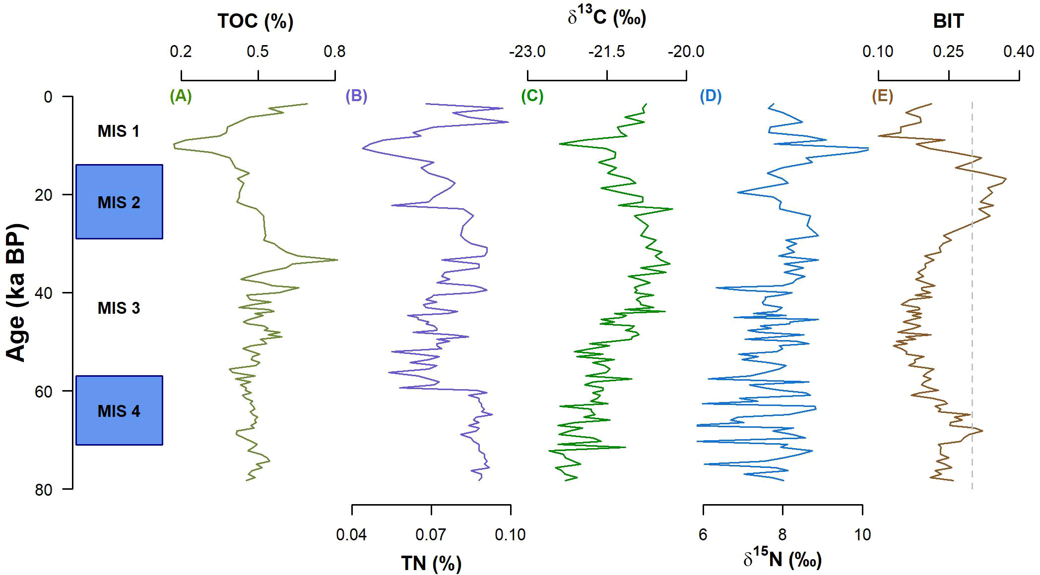
Figure 3 Records of the elemental (A, B) and isotopic (C, D) composition, and BIT values (E) for core NAP 63-1. MIS, Marine Isotope Stage.

The δ¹³C varied between −22.6‰ and −20.3‰ (mean = −21.4‰ ± 0.6) (Figure 3C) and the δ¹⁵N ranged from 5.57‰ to 10.33‰ (mean = 7.87‰ ± 0.76) (Figure 3D). Values of δ¹³C also indicated the predominance of marine OM (δ¹³C = −22‰–−20‰; Meyers, 1994) and were in the same range as observed in SBB surface sediments (δ¹³C = −21.0‰–−20.5‰; Mahiques et al., 2004). The δ¹⁵N values varied slightly throughout the core but remained approximately 7.5‰, reinforcing the marine and/or microbial nature of the OM (Meyers, 1997) (Supplementary Figure S1). The overall low BIT values (mean = 0.22 ± 0.06) corroborate the mainly marine OM source (BIT< 0.3; Hopmans et al., 2004).

Overall, δ¹³C and BIT values indicate a predominance of marine primary production. Specially between 80 and 40 ka BP, a decreasing BIT trend (Figure 3E) coupled to increasing δ¹³C values (Figure 3C) suggests a reduced input from terrestrial sources, either from soil (δ¹³C = −27‰–−23‰; Bianchi and Canuel, 2011) or vascular plants (δ¹³C = −30‰–−26‰; Bianchi and Canuel, 2011). However, during MIS (Marine Isotope Stage) 2 (approximately 20 ka BP), BIT values exceeded the threshold of 0.3 for terrestrial input (Hopmans et al., 2004). It coincided with an excursion toward more negative δ¹³C values, corroborating a slight increase in the contribution of terrestrial OM to the region.

During the Holocene, from 11 ka BP to the present, the TOC content increased. The increasing trend of BIT values suggests that this TOC increase was related to terrestrial rather than marine OM sources. This TOC increase could be caused by a higher terrestrial OM input in response to higher precipitation in southeast America and the expansion of the Atlantic rainforest (Ledru et al., 2009). However, it should have resulted in a decrease in δ¹³C values toward more negative values (δ¹³C from vascular plants = −30‰–−26‰; Bianchi and Canuel, 2011), which is not observed. Possible sources of terrestrial OM with less negative values include plants with C4 and CAM photosynthetic metabolism, such as grasses and plants from tropical regions (Muccio and Jackson, 2009; Chen and Blankenship, 2021). During the last 10 ka, Ledru et al. (2009) observed an expansion of Asteraceae tubuliflorae (C4 metabolism), Ericacea, and Isoetes (both with CAM metabolism) in SE Brazil. Their contribution could explain the relative increase in the terrestrial contribution to the OM input in the sampling region, but without decreasing δ¹³C values.

Marine OM

According to the cluster using SAX representation, 12 compounds were assigned to have a marine source: long-chain even-numbered n-alkanols (n-C₂₀-OH – n-C₃₄-OH), phytol, crenarchaeol, LCA, C₂₈ and C₃₀ 1,14-diols, and the sterols 27Δ^5,22E, 27Δ⁵, 28Δ^5,22E, 28Δ⁵, 29Δ^5,22E, 29Δ⁵, and 30^Δ22E (Dauner et al., 2020) (Figure 2). The long-chain even-numbered n-alkanols are also usually attributed to input from higher plant waxes, but some aquatic sources have also been suggested. Sinninghe Damsté et al. (2001) argued that the most probable marine source of long-chain n-alkanols in Antarctic saltwater lakes is the hydrolysis of cyanobacterial glycolipids.

The constrained cluster analysis allowed us to establish four marine zones (MZs): MZ-I: 79–50 ka BP; MZ-II: 50–39 ka BP; MZ-III: 39–29 ka BP; MZ-IV: 29–2 ka BP (Figure 4). During MZ-I, a relatively high input of 28Δ^5,22E, 30Δ^22E, and phytol was observed, especially during MIS 4 (71–57 ka BP), when compared to other MZs. The MZ-II is characterized by the highest accumulation rates of marine OM proxies (Figure 4). Several studies also observed a peak in the productivity of dinoflagellate and benthic and planktonic foraminifera in the SW Atlantic (e.g., Behling et al., 2002; Almeida et al., 2015; Portilho-Ramos et al., 2015) during this time interval. The marine productivity during MZ-III diminished slightly, returning to values similar to MZ-I, suggesting that at least one of the two fertilization processes observed during MZ-II (discussed below) diminished. The MZ-IV is characterized by the lowest accumulation rates of marine OM proxies (Figure 4).

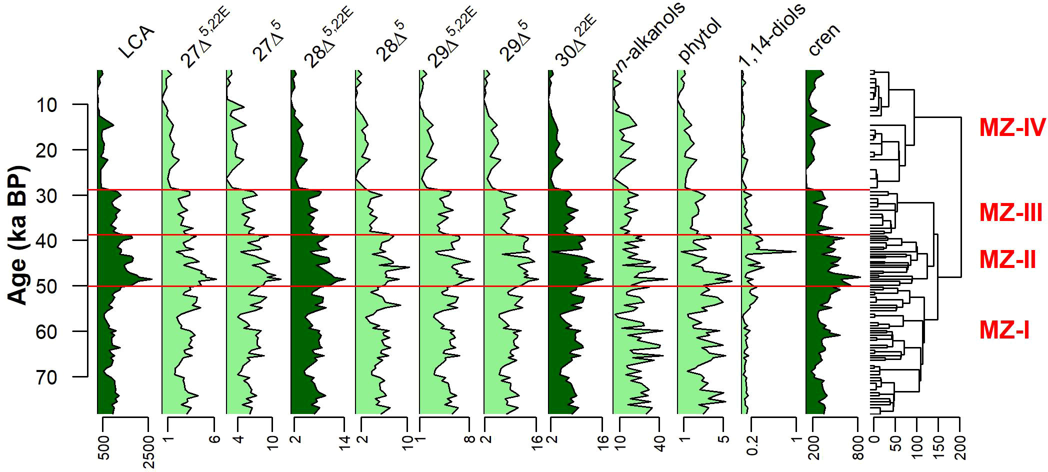
Figure 4 Summary diagram showing the mass accumulation rates (in ng cm⁻² year⁻¹) of the organic molecular markers associated with marine organic matter, the constrained dendrogram, and the MZs for core NAP 63-1. Proxies colored with dark green will be discussed in more detail.

Terrestrial OM

According to the cluster using SAX representation, four compound groups were assigned to have a terrestrial source: mid-chain odd-numbered n-alkanes (n-C₁₉ – n-C₂₃), long-chain odd-numbered n-alkanes (n-C₂₅ – n-C₃₉), short-chain even-numbered n-alkanols (n-C₁₂-OH – n-C₁₈-OH), and brGDGTs (Dauner et al., 2020) (Figure 2). The short-chain n-alkanols were predominant in the n-alkanols, especially the n-C₁₆-OH, which alone accounted for approximately 50% of the total n-alkanols. Usually, aquatic algae and bacteria have n-alkanol distributions dominated by C₁₆ to C₂₂ components (Meyers, 2003). However, Hu et al. (2009) observed a high correlation of short-chain n-alkanols with terrestrially derived bacterial fatty acids, indicating a bacterial source, instead of aquatic algae for the former compounds. In our samples, a high correlation between short-chain n-alkanols and brGDGTs (R = 0.58; α< 0.05) suggests a terrestrial microbial origin for the short-chain n-alkanols.

The constrained cluster analysis allowed us to establish four terrestrial zones (TZ): TZ-I: 79.0–65.5 ka BP; TZ-II: 65.5–32 ka BP; TZ-III: 32.0–29 ka BP; TZ-IV: 29–2 ka BP (Figures 5D-H). During TZ-I, a relatively high input of mid-chain n-alkanes and brGDGTs and low MAR of long-chain n-alkanes were observed. The TZ-II was marked by low MAR of both mid- and long-chain n-alkanes, but with oscillating inputs of short-chain n-alkanols and brGDGTs. The short TZ-III layer was marked by a sharp increase in the n-alkanes MAR and continuously high n-alkanols and brGDGTs MAR. Lastly, TZ-IV was marked by the largest inputs of all terrestrial markers, especially approximately 20 ka BP.

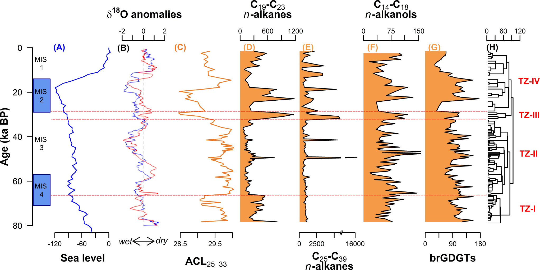
Figure 5 (A) Global sea level evolution (in m) (Miller et al., 2005). (B) Anomalies of δ¹⁸O from the Botuverá (red) and Santana (blue) caves (Cruz et al., 2005; Cruz et al., 2007). (C) n-alkane ACL_25-33 index from NAP 63-1 core. (D-G) Summary diagram showing the mass accumulation rates (in ng cm⁻² year⁻¹) of the organic molecular markers associated with terrestrial organic matter, (H) the constrained dendrogram, and the terrestrial zones (TZ) for core NAP 63-1.

Controls on OM input

OM input to the SBB may have been controlled by multiple mechanisms. Here, we consider variations in precipitation, wind patterns, ocean circulation, and the Si cycle.

Precipitation over the adjacent continent and consequent runoff have been reported to be the main processes that govern the delivery of terrestrial OM and nutrients to the SBB (Nagai et al., 2014b). Cruz et al., 2005; Cruz et al., 2007 studied rainfall variations in southern and SE Brazil through the δ¹⁸O composition of speleothems in Botuverá and Santana caves, respectively (Figure 5B). Wet climate periods observed in southern and SE Brazil coincided with the high MAR of brGDGTs and n-alkanols in the NAP 63-1 record, especially approximately 48 and 20 ka BP. As discussed before, both proxies are associated with terrestrially derived OM. Thus, increased precipitation could have increased soil erosion, increasing the input of soil-derived OM to the SBB. Variations in sea level likely emphasized the precipitation influence. During TZ-I, sea level dropped (Miller et al., 2005; Figure 5A) and, consequently, the continental shelf shortened, reducing the distance to the coast of the core site (from about 170 km, during MIS 5e, to about 40 km, during TZ-I). The shorter distance to the coast, coupled with the wet climate, may explain the relatively high terrestrial OM input in the SBB slope during TZ-I. Between TZ-II and TZ-III, sea level remained at approximately 85 m below the present one, without significant variation.

TZ-III was a short period marked by high MAR of all four terrestrial OM proxies. This period was marked by a slight change to more humid conditions (Figure 5B) but not so expressive that it could explain the terrestrial OM input. A possible explanation is a northward migration of the southern westerly wind belt. Razik et al. (2015) found sediments from the South America Pampas in SBB and related them with northward transport by westerly winds. Large dust flux observed in East Antarctica (Lambert et al., 2008) and high Pb isotope ratios observed in the Eastern Equatorial Pacific (Pichat et al., 2014) approximately 30 ka BP suggest a northward extension of the South Westerly wind belt. This northward migration may have enhanced the eolian transport of terrestrial material to the SBB, as also observed by Mathias et al. (2021).

At the beginning of the TZ-IV, the sea level fell to its minimum, reaching about 120 m below the present level (Miller et al., 2005; Figure 5A). During this period, the continental shelf reached its minimum length, further decreasing the distance to the coast of the core site and increasing the terrestrial input to site NAP 63-1. BIT values higher than 0.3 (Figure 3E) confirm this larger influence of terrestrial OM. During the last deglaciation (19 – 11 ka BP), rapid sea level rise caused the widening of the continental shelf (Figure 5A), which reduced the terrestrial input to the slope.

The n-alkanes, on the other hand, did not present a direct response to precipitation variations (Figures 5D, E). Instead, they could have been more influenced by the vegetation type in the adjacent continent. Badewien et al. (2015) studied vegetation changes of SW Africa during the last 60 ka and found a relation between the ACL values and forest pollen. During periods when forest pollen was highest, ACL values decreased. In the NAP 63-1 record (Figure 5C), the periods of relatively low ACL_25-33 occurred approximately 50 ka BP, between 30 and 20 ka BP, and in the last 10 ka BP.

The use of the ACL as a proxy for woody/forest vs. grassland vegetation is very controversial. Studying the SE Atlantic, Rommerskirchen et al. (2003) observed that marine sediments that receive material from the Congo rain forest tend to present the n-C₂₉ as the main n-alkane. However, marine sediments located further south and receiving material from the savannah tend to present the n-C₃₁ as the main n-alkane. Therefore, they associated the higher ACL values with plants with a C4 metabolism, like grasslands, herbs, and shrubs. More recently, some studies of the alkane composition in leaves from modern plants (Bush and McInerney, 2013; Feakins et al., 2016) did not find a direct correlation between the n-alkane distributions (especially the predominance of n-C₂₉ or n-C₃₁) and the type of vegetation (grasses or woody plants). Bush and McInerney (2013) argued that the pattern observed in the western African coast might reflect the differences in rainforest and savanna environments, rather than in the leaf wax compositions. Nevertheless, the periods of relatively low ACL_25-33 observed in the NAP 63-1 records coincide with periods of a high percentage of arboreal pollen observed in a crater in SE Brazil, located only a few kilometers from the shoreline (Colônia crater; 23°52′S 46°42’20’’ W; Ledru et al., 2009). The dominance of grasslands during the rest of the period was attributed by Gu et al. (2017) to the expansion of salt marshes to the North and over the exposed continental shelf. Thus, for the SBB, it may be possible to use ACL as a proxy for the changes in the Atlantic rainforest in southern and SE Brazil, with lower ACL suggesting an expansion of the rainforest.

The influence of continental precipitation can also be seen in the marine productivity. In the southern portion of SBB, Gu et al. (2017) observed high relative abundances of eutrophic environmental dinocysts and associated them with the enhanced presence of fluvial waters during MZ-I. As shown in Figure 6A, wet climates (low δ¹⁸O values) coincided with an increase in marine productivity in the central portion of the SBB during MIS 4 (approximately 65 ka BP) and during the MZ-II. These coincidences could be explained by fertilization of SBB due to increased fluvial nutrient input driven by wet climate. The spike in marine productivity approximately 16 ka BP may correspond to the wet climate during Heinrich Stadial 1 (between 18.0 and 15.6 ka BP; Campos et al., 2019). Conversely, the dryer climate during MZ-III may have decreased the fluvial input of nutrients to the SBB, causing a slight decrease in marine productivity during this period.

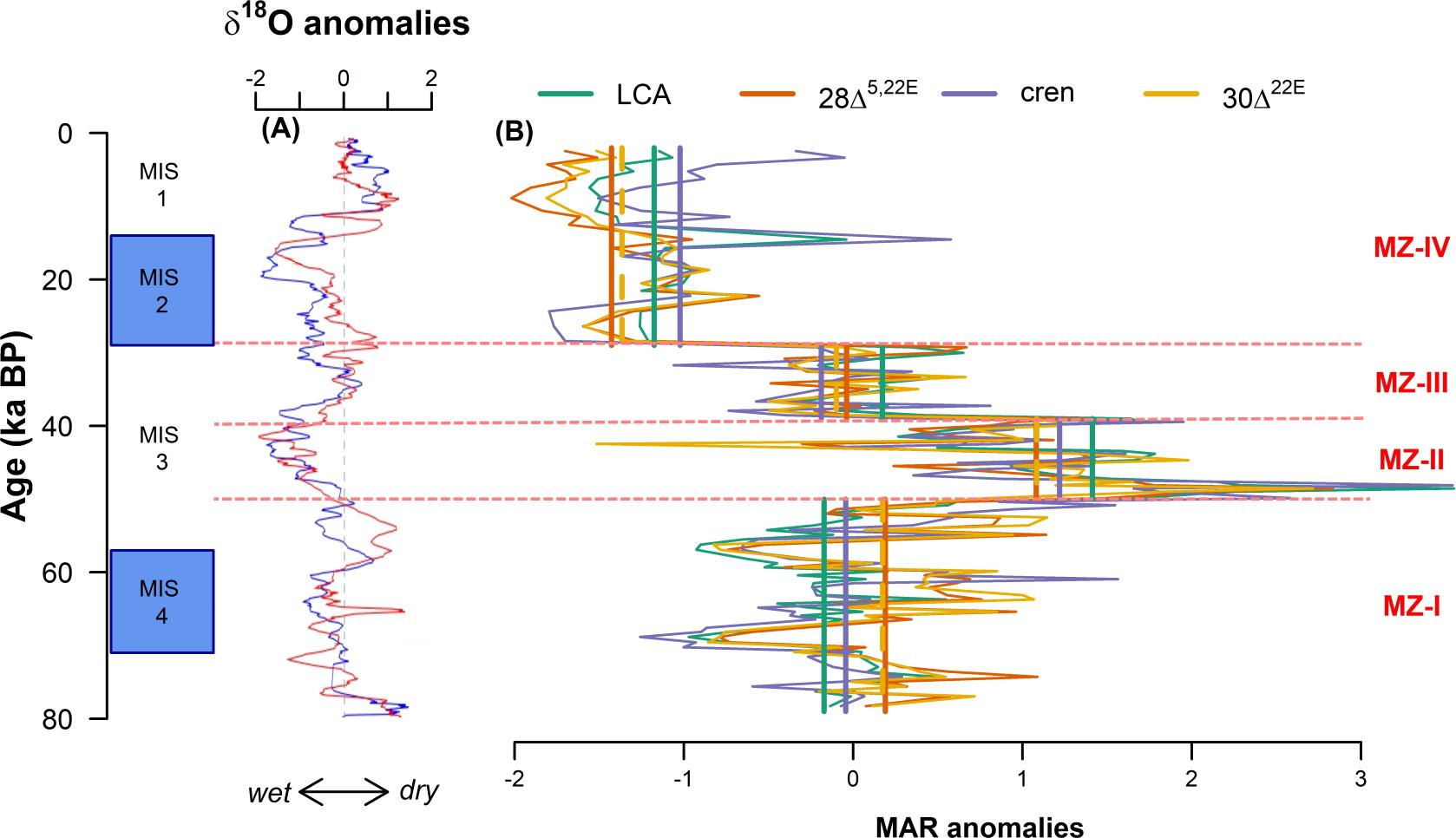
Figure 6 (A) Anomalies of δ¹⁸O from the Botuverá and Santana caves (Cruz et al., 2005; Cruz et al., 2007) and (B) anomalies of the mass accumulation rates (MAR) of long-chain alkenones (LCA), 28Δ^5,22E, crenarchaeol (cren), and 30Δ^22E from the sediment core NAP 63-1. MZ, marine zone. Bold straight lines in (B) refer to the average of each proxy for each MZ.

Marine productivity in the region is also influenced by upwelling of SACW, which in turn is affected by sea level changes. A MIS 3 high stand was reported in the southern Brazilian coast (Salvaterra et al., 2017; Dillenburg et al., 2019). This sea level rise would be responsible for the landward displacement of the whole water masses system (Mahiques et al., 2007), including the nutrient-rich SACW, seasonally upwelled into the area leading to enhanced productivity. The SACW upwelling in the SBB may also be driven by BC cyclonic meanders (Souza et al., 2020). Regardless of the mechanism that promoted the larger intrusion of SACW in the SBB, upwelling of SACW has been suggested to promote marine productivity by planktonic foraminifera in the same sediment core (NAP 63-3; Alvarenga et al., 2022), and at the slopes of the Campos Basin (GL-74 sediment core, 1279 m water column) (Portilho-Ramos et al., 2015) and the southern SBB (GeoB 2107-3 sediment core, 1,048-m water column) (Pereira et al., 2018). To assess whether SACW upwelling was indeed forcing marine productivity variations during the MZ-II and MZ-III, we computed the cross-wavelet between the stable carbon isotope from surface dwelling foraminifera (GL-1090; Nascimento et al., 2021) and the 28Δ^5,22E accumulation rates. This analysis reveals common high energy in the range of 8 ka between 50 and 30 ka BP, with both signals in antiphase, i.e., low δ¹³C and, consequently, more OM regeneration and nutrients coincide with increased 28Δ^5,22E accumulation rates (Figure 7). This same relationship was observed between GL-1090 planktonic δ¹³C and the other marine productivity proxies, such as 30Δ^22E, LCA, and crenarchaeol (not shown). This result supports the hypothesis that SACW upwelling may have fertilized the SBB, boosting marine productivity in the MZ-II and III. The difference in marine productivity observed in these two periods may be explained by the combination of precipitation and SBB upwelling. Between 50 and 40 ka BP, the combination of enhanced SACW upwelling and precipitation may have caused high marine productivity observed during MZ-II. In contrast, although the influence of the SACW was still observed between 40 and 30 ka BP, the dryer climate may have caused the decrease in the marine productivity observed in MZ-III.

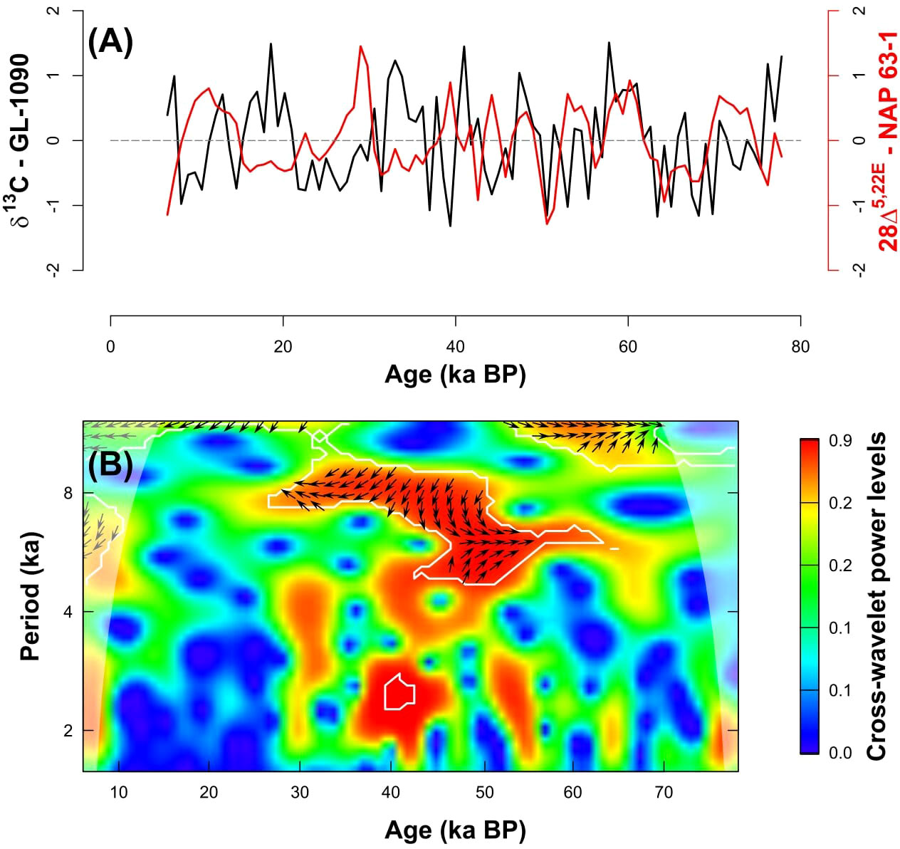
Figure 7 (A) Normalized time series of the stable carbon isotope from thermocline-dwelling foraminifera Globorotalia inflata from sediment core GL-1090 (black line) (Nascimento et al., 2021) and 28Δ^5,22E accumulation rates (ng cm⁻² year⁻¹; blue line) and (B) cross-wavelet analysis between them. The phase arrows in the cross-wavelet power spectrum rotate clockwise with a “north” origin. The vectors indicate the phase relationship, where in-phase signals point upward (N), and antiphase signals point downward (S). If X (δ¹³C) leads Y (28Δ^5,22E), arrows point to the right (E), and if X lags Y, an arrow points to the left (W). Marked regions on the wavelet spectrum indicate significant power to a 95% confidence interval, and areas under the translucid cone of influence show where edge effects are important, and the analysis is unreliable.

From 30 ka BP onward, the relationship between subsurface temperature and other marine productivity proxies becomes variable indicating decoupling between SACW and marine OM proxies (Figure 7). Several studies from the SW Atlantic also observed a decrease in marine productivity (Almeida et al., 2015; Portilho-Ramos et al., 2015; Gu et al., 2017; Pereira et al., 2018; Alvarenga et al., 2022) during this period. The dryer climate coupled with lesser influence of SACW in the SBB, which favors the oligotrophic tropical water in the region, may have caused this substantial decline in marine productivity.

One last explanation for high marine productivity during glacial periods in tropical and subtropical regions is a mechanism related to the silicic acid leakage hypothesis (Brzezinski et al., 2002; Matsumoto et al., 2002). During glacial and dry periods, additions of Fe around Antarctica caused the uptake ratios of Si(OH)₄:NO₃− by diatoms to decline from 4:1 to 1:1 (Brzezinski et al., 2002). Some of the Si excess was then leaked out to lower latitudes through Sub-Antarctic Mode Water (Matsumoto et al., 2002) and may have caused diatoms to displace coccolithophores at low latitudes (Brzezinski et al., 2002). In the South Atlantic, the Sub-Antarctic Mode Water is carried northward by the Malvinas Current and, when it encounters the BC near 39°S, the water downwells, thus forming SACW (Piola and Matano, 2017). In addition to Fe input, sea-ice expansion and the weakening of the southern westerlies may have also promoted Si leakage from the Southern Ocean (Matsumoto et al., 2014). Griffiths et al. (2013) observed an increase in the opal content in the eastern equatorial Atlantic (core RC24-01; 0°33′N, 13°39′W; 3,837-m water depth) during MIS 4 and associated it with a Si-enriched Antarctic Intermediate Water. However, the silicic acid leakage hypothesis should be verified not only by an increase in the diatom productivity but also by a shift of the phytoplankton composition in favor of diatoms over calcite-secreting coccolithophores (Matsumoto et al., 2002). During MIS 4, the average MAR anomaly of 28Δ^5,22E (proxy for diatoms; bold orange line in Figure 6B) during MZ-I is higher than the average MAR anomaly of LCA (a proxy for coccolithophores; bold green line in Figure 6B) for the same period. However, during MIS 2, the MAR anomaly of LCA is higher than the 28Δ^5,22E MAR anomaly. This suggests that the silicic acid leakage may have influenced the marine productivity in the SBB during MIS 4 but not during MIS 2.

Composition of the marine primary producer community

Distinct primary producers characterized the MZs, and Figure 6B summarizes the variations in marine OM productivity and the relationship between these producers. Although differential degradation among different compounds during diagenesis makes it challenging to infer the abundance of living organisms from the biomarker data, their normalized MAR may reflect changes in the contribution of each specific group of organisms (Li et al., 2015). During MZ-I, there was a predominance of diatoms and dinoflagellates, indicated by the concentrations above the long-term mean of 28Δ^5,22E and 30Δ^22E, respectively (Volkman, 1986). A similarity between 28Δ^5,22E and 30Δ^22E contents was also observed by Li et al. (2015), indicating that diatoms and dinoflagellates respond similarly to hydrological variability. During the MZ-II and MZ-III, a relative increase in long-chain alkenones content, biomarkers produced by coccolithophores (Epstein et al., 2001), was observed. Finally, during MZ-IV, a decrease occurred in the contents of the three microalgae proxies. This decrease of the microalgae proxies coincided with an increase in the crenarchaeol accumulation rates, a proxy for Thaumarchaeota (Sinninghe Damsté et al., 2002).

Diatoms are common in eutrophic waters, like coastal regions (Libes, 2009), whereas coccolithophores are usually associated with oligotrophic environments, such as the subtropical gyres (Perrin et al., 2016). Changes in the dominant phytoplankton group are consistent with a shift from a more eutrophic environment during MZ-I to a less nutrient-rich environment during MZ-III. During MZ-I, the surface waters enriched in terrestrially derived nutrients may have favored diatom and dinoflagellate productivity. The hydrodynamic conditions changed entering the MZ-II, and a transient SACW upwelling, driven by BC cyclonic meanders (Almeida et al., 2015), was probably responsible for the relative success of the coccolithophores. The BC cyclonic meanders may have occurred more frequently during this time interval, or the SACW may have reached shallower depths than today.

In the last 20 ka, the decrease in the phytoplankton proxies and increase of the Thaumarchaeota proxies suggest a further decrease in nutrient availability toward the present oligotrophic conditions of the BC (Portilho-Ramos et al., 2015; Lourenço et al., 2016). Thaumarchaeota are a group of chemolithotrophic ammonia-oxidizing archaea, which compete poorly with phytoplankton for nutrients but endure in particularly oligotrophic conditions (Santoro et al., 2019). They can also use organic compounds, such as urea and cyanate, as energy and nitrogen sources (Kitzinger et al., 2019). These abilities allowed the Thaumarchaeota to thrive in the Holocene, becoming an important link in the microbial loop and trophic web of the present BC in the SBB (Moser et al., 2016). In a future warmer scenario, studies using climate and niche models indicate an expansion of oligotrophic regions and replacing larger phytoplankton with smaller organisms (Cabré et al., 2015; Šolić et al., 2018). The picoplankton will probably play an even more important role in the carbon cycle in these situations.

Summary and conclusions

This study highlighted how climate changes affected the sources of OM delivered to the central SBB from the Late Pleistocene to the Holocene. We investigated the primary mechanism controlling marine productivity in the SBB central portion as well as the main delivery routes of the terrestrial OM to the region. According to their temporal evolution, the organic geochemical proxies were classified into “terrestrial-source” and “marine-source” groups. The two OM sources presented distinct stratigraphical zones, indicating distinct mechanisms governing marine OM production and terrestrial OM production and export.

Marine organisms were the primary source of OM for the slope in the last 80 ka. Nutrient input from the adjacent coast seems to have controlled the marine productivity during MZ-I and -II (before 39 ka BP). Upwelling of SACW promoted by the BC cyclonic eddies was likely the primary mechanism controlling marine productivity during MZ-II and -III (between 50 and 29 ka BP). The synergistic effect of terrigenous input and upwelling may have caused the highest marine productivity rates in the Last Glacial Period. In the last 20 ka, a more substantial presence of the oligotrophic tropical water in the region was suggested by a decrease in the phytoplanktonic productivity and a relative increase in archaeal productivity. Due to their ability to use organic compounds and ammonia as energy and nitrogen sources, Thaumarchaeota may have become an important link in the microbial loop and trophic web of the present BC in the SBB.

Stratigraphic zones of the terrestrial OM indicated an oscillating input of soil OM and more sporadic inputs of macrophytes and vascular plants. In general, terrestrial input to the central SBB slope was likely strongly controlled by changes in the continental shelf width and in the type of vegetation over the continent, primarily controlled by sea level fluctuations and the continental moisture evolution, respectively.

Data availability statement

The raw data supporting the conclusions of this article will be made available by the authors, without undue reservation.

Author contributions

MB, MM, and CM designed the concept of the study. AD and JH processed the lipid analyses. AD and GM interpreted the data. AD performed the statistical analysis and wrote the first draft of the manuscript. All authors contributed to manuscript revision, read, and approved the submitted version.

Funding

This study was supported by FAPESP (São Paulo Science Foundation; 2010/06147-5 and 2015/21834-2 research grants) and CNPq (Brazilian National Council for Scientific and Technological Development; 300962/2018-5 and 305763/2011-3 research grants). CM also would like to thank CAPES-PrInt for financial support (88887.311742/2018-00). AD would like to thank Helsinki University Library for the financial support for open access publication fees.

Acknowledgments

AD would like to thank CAPES (Coordenação de Aperfeiçoamento de Pessoal de Ensino Superior) for the Ph.D. Scholarship and Dr. Cristiano Chiessi for the constructive comments.

Conflict of interest

The authors declare that the research was conducted in the absence of any commercial or financial relationships that could be construed as a potential conflict of interest.

Publisher’s note

All claims expressed in this article are solely those of the authors and do not necessarily represent those of their affiliated organizations, or those of the publisher, the editors and the reviewers. Any product that may be evaluated in this article, or claim that may be made by its manufacturer, is not guaranteed or endorsed by the publisher.

Supplementary material

The Supplementary Material for this article can be found online at: https://www.frontiersin.org/articles/10.3389/fmars.2022.924556/full#supplementary-material

References

Almeida F. F. M., Carneiro C. D. R. (1998). Origem e evolução da Serra do Mar. Rev. Bras. Geociências 28, 135–150. doi: 10.5327/rbg.v28i2.617
Almeida F. K., de Mello R. M., Costa K. B., Toledo F. A. L. (2015). The response of deep-water benthic foraminiferal assemblages to changes in paleoproductivity during the pleistocene (last 769.2 kyr), western South Atlantic ocean. Palaeogeogr. Palaeoclimatol. Palaeoecol. 440, 201–212. doi: 10.1016/j.palaeo.2015.09.005
Alvarenga A., Paladino Í.M., Gerotto A., DeMenocal P., Iwai F. S., Sousa S. H. M., et al. (2022). S/SE Brazilian continental margin sea surface temperature and productivity changes over the last 50 kyr. Palaeogeogr. Palaeoclimatol. Palaeoecol. 601, 111144. doi: 10.1016/j.palaeo.2022.111144
Badewien T., Vogts A., Dupont L., Rullkötter J. (2015). Influence of late pleistocene and Holocene climate on vegetation distributions in southwest Africa elucidated from sedimentary n-alkanes - differences between 12°S and 20°S. Quat. Sci. Rev. 125, 160–171. doi: 10.1016/j.quascirev.2015.08.004
Behling H., Arz H. W., Jürgen P., Wefer G. (2002). Late quaternary vegetational and climate dynamics in southeastern Brazil, inferences from marine cores GeoB 3229-2 and GeoB 3202-1. Palaeogeogr. Palaeoclimatol. Palaeoecol. 179, 227–243. doi: 10.1016/S0031-0182(01)00435-7
Bianchi T. S., Canuel E. A. (2011). Chemical biomarkers in aquatic ecosystems (Woodstock, Oxfordshire: Princeton University Press).
Bianchi T. S., Cui X., Blair N. E., Burdige D. J., Eglinton T. I., Galy V. (2018). Centers of organic carbon burial and oxidation at the land-ocean interface. Org. Geochem. 115, 138–155. doi: 10.1016/j.orggeochem.2017.09.008
Blaauw M., Christen J. A. (2011). Flexible paleoclimate age-depth models using an autoregressive gamma process. Bayesian Anal. 6, 457–474. doi: 10.1214/11-BA618
Brzezinski M. A., Pride C. J., Franck V. M., Sigman D. M., Sarmiento J. L., Matsumoto K., et al. (2002). A switch from Si(OH)4 to NO3- depletion in the glacial southern ocean. Geophys. Res. Lett. 29, 1–4. doi: 10.1029/2001GL014349
Bush R. T., McInerney F. A. (2013). Leaf wax n-alkane distributions in and across modern plants: Implications for paleoecology and chemotaxonomy. Geochim. Cosmochim. Acta 117, 161–179. doi: 10.1016/j.gca.2013.04.016
Cabré A., Marinov I., Leung S. (2015). Consistent global responses of marine ecosystems to future climate change across the IPCC AR5 earth system models. Clim. Dyn. 45, 1253–1280. doi: 10.1007/s00382-014-2374-3
Campos M. C., Chiessi C. M., Prange M., Mulitza S., Kuhnert H., Paul A., et al. (2019). A new mechanism for millennial scale positive precipitation anomalies over tropical south America. Quat. Sci. Rev. 225:1–13. doi: 10.1016/j.quascirev.2019.105990
Campos E. J. D., Velhote D., Silveira I. C. A. (2000). Shelf break upwelling driven by Brazil current cyclonic meanders. Geophys. Res. Lett. 27, 751–754. doi: 10.1029/1999GL010502
Chen M., Blankenship R. E. (2021). ““Photosynthesis | photosynthesis,”,” in Encyclopedia of biological chemistry III. Ed. Jez J. (Oxford: Elsevier), 150–156. doi: 10.1016/B978-0-12-819460-7.00081-5
Costa K. B., Cabarcos E., Santarosa A. C. A., Battaglin B. B. F., Toledo F. A. L. (2016). A multiproxy approach to the climate and marine productivity variations along MIS 5 in SE Brazil: A comparison between major components of calcareous nannofossil assemblages and geochemical records. Palaeogeogr. Palaeoclimatol. Palaeoecol. 449, 275–288. doi: 10.1016/j.palaeo.2016.02.032
Cruz F. W. Jr., Burns S. J., Jercinovic M., Karmann I., Sharp W. D., Vuille M. (2007). Evidence of rainfall variations in southern Brazil from trace element ratios (Mg/Ca and Sr/Ca) in a late Pleistocene stalagmite. Geochim. Cosmochim. Acta 71, 2250–2263. doi: 10.1016/j.gca.2007.02.005
Cruz F. W. Jr., Burns S. J., Karmann I., Sharp W. D., Vuille M., Cardoso A. O., et al. (2005). Insolation-driven changes in atmospheric circulation over the past 116,000 years in subtropical Brazil. Lett. Nat. 434, 63–66. doi: 10.1029/2003JB002684
Dauner A. L. L., Mollenhauer G., Bícego M. C., Martins C. C. (2020). Cluster analysis for time series based on organic geochemical proxies. Org. Geochem. 145, 104038. doi: 10.1016/j.orggeochem.2020.104038
Dauner A. L. L., Mollenhauer G., Bícego M. C., Souza M. M., Nagai R. H., Figueira R. C. L., et al. (2019). Multi-proxy reconstruction of sea surface and subsurface temperatures in the western south Atlantic over the last ~ 75 kyr. Quat. Sci. Rev. 215, 22–34. doi: 10.1016/j.quascirev.2019.04.020
Dillenburg S. R., Barboza E. G., Rosa M. L. C. C., Caron F., Cancelli R., Santos-Fischer C. B., et al. (2019). Sedimentary records of marine isotopic stage 3 (MIS 3) in southern Brazil. Geo-Mar. Lett. 40, 1099–108. doi: 10.1007/s00367-019-00574-2
Epstein B. L., D’Hondt S., Hargraves P. E. (2001). The possible metabolic role of C37 alkenones in emiliania huxleyi. Org. Geochem. 32, 867–875. doi: 10.1016/S0146-6380(01)00026-2
Faux J. F., Belicka L. L., Rodger Harvey H. (2011). Organic sources and carbon sequestration in Holocene shelf sediments from the western Arctic ocean. Cont. Shelf. Res. 31, 1169–1179. doi: 10.1016/j.csr.2011.04.001
Feakins S. J., Peters T., Wu M. S., Shenkin A., Salinas N., Girardin C. A. J., et al. (2016). Production of leaf wax n-alkanes across a tropical forest elevation transect. Org. Geochem. 100, 89–100. doi: 10.1016/j.orggeochem.2016.07.004
Garzoli S. L., Matano R. P. (2011). The south Atlantic and the Atlantic meridional overturning circulation. Deep. Res. Part II Top. Stud. Oceanogr. 58, 1837–1847. doi: 10.1016/j.dsr2.2010.10.063
Griffiths J. D., Barker S., Hendry K. R., Thornalley D. J. R., Van De Flierdt T., Hall I. R., et al. (2013). Evidence of silicic acid leakage to the tropical Atlantic via Antarctic intermediate water during marine isotope stage 4. Paleoceanography 28, 307–318. doi: 10.1002/palo.20030
Gu F., Zonneveld K. A. F., Chiessi C. M., Arz H. W., Jürgen P., Behling H. (2017). Long-term vegetation, climate and ocean dynamics inferred from a 73,500 years old marine sediment core (GeoB2107-3) off southern Brazil. Quat. Sci. Rev. 172, 55–71. doi: 10.1016/j.quascirev.2017.06.028
Holland A. R., Petsch S. T., Castañeda I. S., Wilkie K. M., Burns S. J., Brigham-Grette J. (2013). A biomarker record of lake El’gygytgyn, far East Russian Arctic: Investigating sources of organic matter and carbon cycling during marine isotope stages 1-3. Clim. Past 9, 243–260. doi: 10.5194/cp-9-243-2013
Hopmans E. C., Weijers J. W. H., Schefuß E., Herfort L., Sinninghe Damsté J. S., Schouten S. (2004). A novel proxy for terrestrial organic matter in sediments based on branched and isoprenoid tetraether lipids. Earth Planet. Sci. Lett. 224, 107–116. doi: 10.1016/j.epsl.2004.05.012
Hu J., Peng P., Chivas A. R. (2009). Molecular biomarker evidence of origins and transport of organic matter in sediments of the Pearl river estuary and adjacent South China Sea. Appl. Geochem. 24, 1666–1676. doi: 10.1016/j.apgeochem.2009.04.035
Juggins S. (2017). Rioja: Analysis of quaternary science data. r package version 0.9-15.1. 58. Available at: https://cran.r-project.org/web/packages/rioja/index.html.
Kitzinger K., Padilla C. C., Marchant H. K., Hach P. F., Herbold C. W., Kidane A. T., et al. (2019). Cyanate and urea are substrates for nitrification by Thaumarchaeota in the marine environment. Nat. Microbiol. 4, 234–243. doi: 10.1038/s41564-018-0316-2
Lambert F., Delmonte B., Petit J. R., Bigler M., Kaufmann P. R., Hutterli M. A., et al. (2008). Dust - climate couplings over the past 800,000 years from the EPICA dome c ice Core. Nature 452, 616–619. doi: 10.1038/nature06763
Ledru M. P., Mourguiart P., Riccomini C. (2009). Related changes in biodiversity, insolation and climate in the Atlantic rainforest since the last interglacial. Palaeogeogr. Palaeoclimatol. Palaeoecol. 271, 140–152. doi: 10.1016/j.palaeo.2008.10.008
Ligges U., Short T., Kienzle P., Schnackenberg S., Billinghurst D., Borchers H.-W., et al. (2021) Signal: Signal processing. r package version 0.7-7. Available at: https://cran.r-project.org/web/packages/signal/signal.pdf.
Li L., Li Q., He J., Wang H., Ruan Y., Li J. (2015). Biomarker-derived phytoplankton community for summer monsoon reconstruction in the western south China Sea over the past 450ka. Deep. Res. Part II Top. Stud. Oceanogr. 122, 118–130. doi: 10.1016/j.dsr2.2015.11.006
Lin J., Keogh E., Wei L., Lonardi S. (2007). Experiencing SAX: A novel symbolic representation of time series. Data Min. Knowl. Discov 15, 107–144. doi: 10.1007/s10618-007-0064-z
Lisiecki L. E., Raymo M. E. (2005). A pliocene-pleistocene stack of 57 globally distributed benthic δ18O records. Paleoceanography 20, 1–17. doi: 10.1029/2004PA001071
Lisiecki L. E., Stern J. V. (2016). Regional and global benthic δ18O stacks for the last glacial cycle. Paleoceanography 31, 1368–1394. doi: 10.1002/2016PA003002
Lourenço R. A., Mahiques M. M., Wainer I. E. K. C., Rosell-Melé A., Bícego M. C. (2016). Organic biomarker records spanning the last 34,800 years from the southeastern Brazilian upper slope: Links between sea surface temperature, displacement of the Brazil current, and marine productivity. Geo-Mar. Lett. 36, 361–369. doi: 10.1007/s00367-016-0453-7
Mahiques M. M., Fukumoto M. M., Silveira I. C. A., Figueira R. C. L., Bícego M. C., Lourenço R. A., et al. (2007). Sedimentary changes on the southeastern Brazilian upper slope during the last 35,000 years. An. Acad. Bras. Cienc. 79, 171–181. doi: 10.1590/S0001-37652007000100018
Mahiques M. M., Hanebuth T. J. J., Nagai R. H., Bícego M. C., Figueira R. C. L., Sousa S. H. M., et al. (2017). Inorganic and organic geochemical fingerprinting of sediment sources and ocean circulation on a complex continental margin (São Paulo bight, Brazil). Ocean Sci. 13, 209–222. doi: 10.5194/os-13-209-2017
Mahiques M. M., Nagai R. H., Dias G. P., Figueira R. C. L. (2022). An 80 kyr record of intermediate-depth water flow on the western south Atlantic margin. Sedimentology, 1–13. doi: 10.1111/sed.13016
Mahiques M. M., Tessler M. G., Ciotti A. M., Silveira I. C. A., Sousa S. H. M., Figueira R. C. L., et al. (2004). Hydrodynamically driven patterns of recent sedimentation in the shelf and upper slope off southeast Brazil. Cont. Shelf. Res. 24, 1685–1697. doi: 10.1016/j.csr.2004.05.013
Mathias G. L., Roud S. C., Chiessi C. M., Campos M. C., Dias B. B., Santos T. P., et al. (2021). A multi-proxy approach to unravel late Pleistocene sediment flux and bottom water conditions in the western South Atlantic ocean. Paleoceanogr. Paleoclimatol. 36, 1–22. doi: 10.1029/2020PA004058
Matsumoto K., Chase Z., Kohfeld K. (2014). Different mechanisms of silicic acid leakage and their biogeochemical consequences. Paleoceanography 29, 238–254. doi: 10.1002/2013PA002588
Matsumoto K., Sarmiento J. L., Brzezinski M. A. (2002). Silicic acid leakage from the southern ocean: A possible explanation for glacial atmospheric pCO2. Global Biogeochem. Cycles 16, 5-1-5–5-123. doi: 10.1029/2001gb001442
Meyers P. A. (1994). Preservation of elemental and isotopic source identification of sedimentary organic matter. Chem. Geol. 114, 289–302. doi: 10.1016/0009-2541(94)90059-0
Meyers P. A. (1997). Organic geochemical proxies of paleoceanographic, paleolimnologic, and paleoclimatic processes. Org. Geochem. 27, 213–250. doi: 10.1016/S0146-6380(97)00049-1
Meyers P. A. (2003). Applications of organic geochemistry to paleolimnological reconstructions: A summary of examples from the Laurentian great lakes. Org. Geochem. 34, 261–289. doi: 10.1016/S0146-6380(02)00168-7
Miller K. G., Kominz M. A., Browning J. V., Wright J. D., Mountain G. S., Katz M. E., et al. (2005). The Phanerozoic record of global sea-level change. Science 310, 1293-1298. doi: 10.1126/science.1116412
Montero P., Vilar J. A. (2014). TSclust: An R package for time series clustering. J. Stat. Software 62, 1–43. doi: 10.18637/jss.v062.i01
Moser G. A. O., Castro N. O., Takanohashi R. A., Fernandes A. M., Pollery R. C. G., Tenenbaum D. R., et al. (2016). The influence of surface low-salinity waters and cold subsurface water masses on picoplankton and ultraplankton distribution in the continental shelf off Rio de Janeiro, SE Brazil. Cont. Shelf. Res. 120, 82–95. doi: 10.1016/j.csr.2016.02.017
Muccio Z., Jackson G. P. (2009). Isotope ratio mass spectrometry. Analyst 134, 213–222. doi: 10.1039/B808232D
Muelbert J. H., Acha M., Mianzan H., Guerrero R., Reta R., Braga E. S., et al. (2008). Biological, physical and chemical properties at the subtropical shelf front zone in the SW Atlantic continental shelf. Cont. Shelf. Res. 28, 1662–1673. doi: 10.1016/j.csr.2007.08.011
Müller P. J. (2004). Density and water content of sediment core GeoB2107-3. doi: 10.1594/PANGAEA.143110
Nagai R. H., Ferreira P. A. L., Mulkherjee S., Martins M. V. A., Figueira R. C. L., Sousa S. H. M., et al. (2014a). Hydrodynamic controls on the distribution of surface sediments from the southeast south American continental shelf between 23° S and 38° S. Cont. Shelf. Res. 89, 51–60. doi: 10.1016/j.csr.2013.09.016
Nagai R. H., Sousa S. H. M., Lourenço R. A., Bícego M. C., Mahiques M. M. (2010). Paleoproductivity changes during the late quaternary in the southeastern Brazilian upper continental margin of the southwestern Atlantic. Braz. J. Oceanogr. 58, 31–41. doi: 10.1590/S1679-87592010000500004
Nagai R. H., Sousa S. H. M., Mahiques M. M. (2014b). ““The southern Brazilian shelf,”,” in Continental shelves of the world: Their evolution during the last glacio-eustatic cycle. Eds. Chiocchi F. L., Chivas A. R. (London: Geological Society), 47–54. doi: 10.1144/M41.5
Nascimento R. A., Santos T. P., Venancio I. M., Chiessi C. M., Ballalai J. M., Kuhnert H., et al. (2021). Origin of δ13C minimum events in thermocline and intermediate waters of the western south Atlantic. Quat. Sci. Rev. 272, 107224. doi: 10.1016/j.quascirev.2021.107224
Oksanen J., Blanchet F. G., Friendly M., Kindt R., Legendre P., McGlinn D., et al. (2018). “Vegan: Community ecology package,” in R package version 2, 5–3. Available at: https://cran.r-project.org/web/packages/vegan/index.html
Pereira L. S., Arz H. W., Pätzold J., Portilho-Ramos R. C. (2018). Productivity evolution in the south Brazilian bight during the last 40,000 years. Paleoceanogr. Paleoclimatol. 33, 1339–1356. doi: 10.1029/2018PA003406
Perrin L., Probert I., Langer G., Aloisi G. (2016). Growth of the coccolithophore Emiliania huxleyi in light- and nutrient-limited batch reactors: Relevance for the BIOSOPE deep ecological niche of coccolithophores. Biogeosciences 13, 5983–6001. doi: 10.5194/bg-13-5983-2016
Pichat S., Abouchami W., Galer S. J. G. (2014). Lead isotopes in the Eastern equatorial pacific record Quaternary migration of the south Westerlies. Earth Planet. Sci. Lett. 388, 293–305. doi: 10.1016/j.epsl.2013.11.035
Piola A. R., Matano R. P. (2017). ““Ocean currents: Atlantic Western boundary - Brazil Current/Falkland (Malvinas) current,”,” in Reference module in earth systems and environmental sciences (Elsevier). doi: 10.1016/B978-0-12-409548-9.10541-X
Portilho-Ramos R. C., Ferreira F., Calado L., Frontalini F., Toledo M. B. (2015). Variability of the upwelling system in the southeastern Brazilian margin for the last 110,000 years. Glob. Planet. Change 135, 179–189. doi: 10.1016/j.gloplacha.2015.11.003
Poynter J., Eglinton G. (1990). Molecular composition of three sediments from hole 717C: The Bengal Fan in Proceedings of the Ocean Drilling Program, Scientific Results, eds. J. R. Cochran, D. A. V. Stow, and et al. (College Station, TX: Ocean Drilling Program), 155–161. doi: 10.2973/odp.proc.sr.116.151.1990
Razik S., Govin A., Chiessi C. M., von Dobeneck T. (2015). Depositional provinces, dispersal, and origin of terrigenous sediments along the SE South American continental margin. Mar. Geol. 363, 261–272. doi: 10.1016/j.margeo.2015.03.001
R Core Team (2021) R: A language and environment for statistical computing. Available at: http://www.r-project.org.
Ribeiro C. G., Lopes dos Santos A., Marie D., Pellizari V. H., Brandini F. P., Vaulot D. (2016). Pico and nanoplankton abundance and carbon stocks along the Brazilian bight. PeerJ 4, e2587. doi: 10.7717/peerj.2587
Ribeiro M. C., Metzger J. P., Martensen A. C., Ponzoni F. J., Hirota M. M. (2009). The Brazilian Atlantic forest: How much is left, and how is the remaining forest distributed? implications for conservation. Biol. Conserv. 142, 1141–1153. doi: 10.1016/j.biocon.2009.02.021
Roesch A., Schmidbauer H. (2018). “WaveletComp: Computational wavelet analysis,” in R package version 1.1, vol. 89. . Available at: https://cran.r-project.org/package=WaveletComp.
Rommerskirchen F., Eglinton G., Dupont L., Güntner U., Wenzel C., Rullkötter J. (2003). A north to south transect of Holocene southeast Atlantic continental margin sediments: Relationship between aerosol transport and compound-specific δ13C land plant biomarker and pollen records. Geochem. Geophys. Geosystems 4:1–29. doi: 10.1029/2003GC000541
Salvaterra A., da S., dos R. F., Salaroli A. B., Figueira R. C. L., Mahiques M. M. (2017). Evidence of an marine isotope stage 3 transgression at the Baixada Santista, south-eastern Brazilian coast. Braz. J. Geol. 47, 693–702. doi: 10.1590/2317-4889201720170057
Santoro A. E., Richter R. A., Dupont C. L. (2019). Planktonic marine archaea. Ann. Rev. Mar. Sci. 11, 131–158. doi: 10.1146/annurev-marine-121916-063141
Sarmiento J. L., Gruber N. (Eds.) (2006). ““Remineralization and burial in the sediments,”,” in Ocean biogeochemical dynamics (Princeton (UK: Princeton University Press), 227–269.
Schaeffer-Novelli Y., Cintrón-Molero G., Adaime R. R., Camargo T. M. (1990). Variability of mangrove ecosystems along the Brazilian coast. Estuaries 13, 204–218. doi: 10.2307/1351590
Silveira I. C. A., Foloni Neto H., Costa T. P., Schmidt A. C. K., Pereira A. F., Castro Filho B. M., et al. (2015). ““Caracterização da oceanografia física do talude continental e região oceânica da Bacia de Campos,”,” in Meteorologia e oceanografia. Eds. Martins R. P., Grossmann-Matheson G. S. (Rio de Janeiro, RJ: Elsevier), 135–189. doi: 10.1016/b978-85-352-6208-7.50011-8
Sinninghe Damsté J. S., Schouten S., Hopmans E. C., van Duin A. C. T., Geenevasen J. A. J. (2002). Crenarchaeol: The characteristic core glycerol dibiphytanyl glycerol tetraether membrane lipid of cosmopolitan pelagic crenarchaeota. J. Lipid Res. 43, 1641–1651. doi: 10.1194/jlr.M200148-JLR200
Sinninghe Damsté J. S., Van Dongen B. E., Rijpstra W. I. C., Schouten S., Volkman J. K., Geenevasen J. A. J. (2001). Novel intact glycolipids in sediments from an Antarctic lake (Ace lake). Org. Geochem. 32, 321–332. doi: 10.1016/S0146-6380(00)00165-0
Šolić M., Grbec B., Matić F., Šantić D., Šestanović S., Ninčević G. Ž., et al. (2018). Spatio-temporal reproducibility of the microbial food web structure associated with the change in temperature: Long-term observations in the Adriatic Sea. Prog. Oceanogr. 161, 87–101. doi: 10.1016/j.pocean.2018.02.003
Souza M. M., Mathis M., Mayer B., Noernberg M. A., Pohlmann T. (2020). Possible impacts of anthropogenic climate change to the upwelling in the South Brazil bight. Clim. Dyn. 55, 651–664. doi: 10.1007/s00382-020-05289-0
Torrence C., Compo G. P. (1998). A practical guide to wavelet analysis. Bull. Am. Meteorol. Soc 79, 61–78. doi: 10.1175/1520-0477(1998)079<0061:APGTWA>2.0.CO;2
Volkman J. K. (1986). A review of sterol markers for marine and terrigenous organic matter. Org. Geochem. 9, 83–99. doi: 10.1016/0146-6380(86)90089-6
Weijers J. W. H., Schefuß E., Schouten S., Sinninghe Damsté J. S. (2007). Coupled thermal and hydrological evolution of tropical Africa over the last deglaciation. Science 315, 1701-1704. doi: 10.1126/science.1138131
Keywords: continental slope, marine productivity, mass accumulation rates, organic proxies, paleoceanography, South Brazil Bight, stratigraphical zones, terrestrial matter
Citation: Dauner ALL, Mollenhauer G, Hefter J, Bícego MC, de Mahiques MM and Martins CdC (2022) Late Pleistocene to Holocene variations in marine productivity and terrestrial material delivery to the western South Atlantic. Front. Mar. Sci. 9:924556. doi: 10.3389/fmars.2022.924556
Received: 20 April 2022; Accepted: 03 August 2022;
Published: 22 August 2022.
Edited by:
Jacek Raddatz, Goethe University Frankfurt, GermanyReviewed by:
André Bahr, Institute of Earth Sciences, Heidelberg University, GermanyTomoko Komada, San Francisco State University, United States
Copyright © 2022 Dauner, Mollenhauer, Hefter, Bícego, de Mahiques and Martins. This is an open-access article distributed under the terms of the Creative Commons Attribution License (CC BY). The use, distribution or reproduction in other forums is permitted, provided the original author(s) and the copyright owner(s) are credited and that the original publication in this journal is cited, in accordance with accepted academic practice. No use, distribution or reproduction is permitted which does not comply with these terms.
*Correspondence: Ana Lúcia Lindroth Dauner, anadauner@gmail.com; César de Castro Martins, ccmart@ufpr.br