Comparison of an In Situ Imaging Device and Net-Based Method to Study Mesozooplankton Communities in an Oligotrophic System

1 Introduction

To understand ocean ecosystems, it is necessary to understand zooplankton community structure. Zooplankton have a wide range of complex life history strategies, body types, and feeding strategies (Kiørboe et al., 2011). Trophic interactions and behavior of zooplankton can have large impacts on the biological carbon pump, and thus the global carbon cycle (Steinberg and Landry 2017). However, zooplankton communities are extremely dynamic, and populations of different plankton can fluctuate largely over fine temporal and spatial scales. Therefore, studying zooplankton populations and communities can be a great challenge.

Historically, zooplankton have been collected using net-based approaches. Mesh nets allow for the concentration of large volumes of water to sample zooplankton and accurately estimate their abundance. Over the past several decades, advances in net technology includes opening and closing net systems, such as the MOCNESS and MultiNet, which allow for the study of zooplankton communities’ vertical structure (Wiebe and Benfield, 2003). However, there are limitations to net-based study of plankton. Specifically, nets can be destructive and do not adequately sample gelatinous or fragile bodied zooplankton. Additionally, even with open-closing net systems, nets do not offer fine enough scales of vertical resolution to study zooplankton which can occur in dense, thin layers (Holliday et al., 2003).

Recently, developments in imaging technology have offered a new way to study zooplankton. In situ imaging tools offer a large advantage over nets because they can sample a plankter’s exact position in the water column. The frequency of image collection can be fairly close to the frequency of data collection for physical parameters. This information allows for the study of plankton in context with small-scale changes in physical features of the water column (Ohman, 2019) and ecological interactions such as thin layers. Furthermore, in situ imaging allows for the characterization of plankton’s natural state and traits, while nets can disturb and damage plankton. In the past several years, plankton ecologists are increasingly utilizing a trait-based approach to characterize zooplankton communities (Litchman et al., 2013; Kiørboe et al., 2018). Recently, there has been advances in combining in situ imaging and trait-based methodology to study zooplankton (Ohman, 2019; Vilgrain et al., 2021; Orenstein et al., 2021). Studying plankton in situ is particularly important for the study of fragile and gelatinous organisms. In situ plankton imaging devices have recently shed light on some of the major community roles that previously under-described taxa have in ocean ecosystems (Biard et al., 2016; Christiansen et al., 2018; Hoving et al., 2019; Stukel et al., 2019).

There are a wide range of tools which facilitate the study of zooplankton in situ. Examples of this technology include the zooglider (Ohman et al., 2018), ISIIS (Cowen and Guiginad, 2008), LOKI (Schulz et al., 2010), LOPC (Herman et al., 2004), PELAGIOS (Hoving et al., 2019), VPR (Davis et al., 1992), and UVP (Picheral et al., 2010; Picheral et al., 2022) (see Lombard et al., 2019 for a complete review of optical tools). Although these tools accomplish a similar goal, they have vastly different approaches and outcomes. Some devices are independently towed (Cowen and Guiginad 2008; Hoving et al., 2019), while others are designed to be incorporated with oceanographic instrument rosettes (Picheral et al., 2010; Picheral et al., 2022). Illumination and imaging technology also varies between devices. Plankton cameras can include white-light (Hoving et al., 2019), single beam and two-beam red-light (Picheral et al., 2010; Picheral et al., 2022), shadowgraphy (Cowen and Guiginad 2008; Ohman et al., 2018), holography (Nayak et al., 2021), dark-field microscopy (Orenstein et al., 2020), and more. Additionally, these devices range in the quality of image taken, frequency of data collection, and volume sampled in a given profile (Lombard et al., 2019). In this paper, we focus on the Underwater Vision Profiler 5 (UVP5; Picheral et al., 2010). The UVP5 has been commercially available for several years and is a popular tool due to its ability to study both particles and zooplankton. Additionally, the UVP is designed to be able to integrate into CTD-rosette instrument packages and collect data semi-autonomously. This allows for collection of data alongside with standard oceanographic research and no additional wire-time. To date, there have been several studies utilizing UVPs to study particles (Forest et al., 2013; Puig et al., 2013; Martin et al., 2013; Jouandet et al., 2014; Miquel et al., 2015; Waite et al., 2016; Turner et al., 2017; Hoving et al., 2020); zooplankton (Forest et al., 2012; Biard et al., 2016; Hauss et al., 2016; Donoso et al., 2017; Christiansen et al., 2018; Vilgrain et al., 2021), and cyanobacteria (Guidi et al., 2012; Sandel et al., 2015). Studies utilizing the UVP have been conducted in a wide range of environments including the Mediterranean (Donoso et al., 2017; Durrieu de Madron et al., 2017; Severin et al., 2017), Equatorial (Kiko et al., 2017), Atlantic (Thomsen et al., 2019; Christiansen et al., 2018), Pacific (Turner et al., 2017; Stukel et al., 2019), Artic (Miquel et al., 2015; Vilgrain et al., 2021) and Antarctic (Martin et al., 2013). However, there are few studies in oligotrophic regions (Sandel et al., 2015).

One challenge of sampling zooplankton in oligotrophic systems is that zooplankton densities are very low. Thus, large volumes of water are required to adequately study their populations. Some studies with the UVP observed that the volume sampled was too low to adequately describe zooplankton populations (Donoso et al., 2017). However, Forest et al. (2012) found that in a copepod dominated system, the UVP can yield similar density estimate to net-based systems. This suggests the need for regional analyses to assess how effective the UVP measurements are compared to net-based systems. Additionally, recent developments in the UVP have made it available with much higher sampling frequencies, facilitating a larger sampling volume. This can increase the reliability of UVP data collection. However, high sampling frequencies also introduce new challenges like double imaging of individual particles.

Overall, the UVP is an attractive choice for studying zooplankton due to its ability to both study organisms in situ as well as the ease of incorporating it into standard sampling programs. However, there is a clear need to assess how UVP estimates of zooplankton populations compare to net-based systems. In the present study, we offer a comparison of zooplankton abundance and biomass calculations using an in situ imaging device (UVP5-HD) and a depth-specific net system (MOCNESS). This study addresses particular challenges working with high-frequency imaging systems and systems with low-organism density. Finally, we describe the reliability of sampling different devices with both devices.

2 Materials and Methods

2.1 Sample Collection

Data were collected onboard the R/V Atlantic Explorer during 5-day cruises as part of the Bermuda Atlantic Time-series Study (BATS; Steinberg et al., 2001), which conducts monthly long-term monitoring sampling ~80 km southeast of Bermuda. This study utilizes data collected during the June and July BATS cruises of 2019 (AE1912 and AE1917 respectively).

2.1.1 In Situ Imaging of Plankton

An Underwater Vision Profiler (UVP5-HD, sn:209, Hydroptic, Picheral et al., 2010) was attached to the CTD Rosette aboard the R/V Atlantic Explorer. This model of the UVP5-HD has a 4.2-megapixel camera which images a 3.11cm x 18.8 cm x 18.8cm (H x W x L) field of view (1.1L). The pixel size is 92μm. The UVP is designed to measure both particle abundances and collect in situzooplankton imagery. Under mixed acquisition mode, the UVP automatically segments and measures all particles larger than 125μm according to equivalent spherical diameter (ESD). All particles larger than 500μm ESD were recorded and stored as individual images (vignettes). Images are collected at a rate of approximately 15Hz.

The UVP was attached to the CTD rosette on all cruises and configured for automatic acquisition of data for all profiles during each cruise (~18 casts per cruise). On average, a UVP cast sampled 9.31m³ in the epipelagic (0-250m) and 14.38m³ in the mesopelagic (250m-1000m) (Table 1; Supplemental Figure 1; Supporting Information). Images are collected during down casts only, then the UVP is programmed to turn off once it has ascended more than 30m. Data are downloaded from the UVP onboard then processed in Zooprocess and trimmed to remove any data collected during the rinse cycle or the first 30m of the upcast. UVP data are then uploaded to the EcoPart web application (Picheral et al., 2017; https://ecopart.obs-vlfr.fr/), which applies a descent filter to account for variation in the data from ship rock or variable CTD descent speeds. The descent filter excludes any images which were taken at a shallower depth than the preceding image. However, UVP images can still overlap if the UVP is descending at a slow enough rate (<0.622ms^-1; Supplemental Figure 1). The average UVP descent rate in the epipelagic was 0.653ms^-1 and 1.099ms^-1 in the mesopelagic. We did find that at the bottom 50m of each profile, the slowing of the CTD rosette could lead to the high potential of re-imaging particles (Supplemental Figure 1). To account for this, we removed data collected from the bottom 50m of each profile. The typical UVP cast descended to 1200m, although several descended to approximately 500m. Consequently, the removal of the bottom 50m has minimal impact on the data available for this analysis.

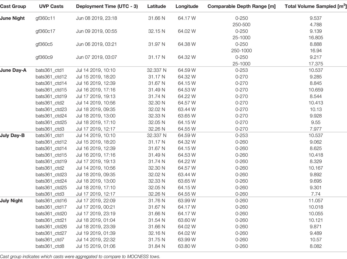
Table 1 Metadata for UVP casts.

2.1.2 Net-Based Plankton Collection

Plankton were collected using a Multiple Opening and Closing Net with Environmental Sensing System (MOCNESS; Wiebe et al., 1976, Wiebe et al., 1985). The MOCNESS has a 1m^-2 opening and was equipped with 153µm mesh and was deployed on oblique tows. The MOCNESS was used to sample plankton at discrete depth-bins following an adaptive profiling method to sample ecologically relevant regions of the water column. Specifically, bins were targeted to capture variation around the deep chlorophyll-a maximum (DCM) which was determined prior to each tow using a CTD cast with an attached fluorometer (Chelsea Instruments). It should be noted that tows between the two cruises did have different maximum depths (Table 2). During the June cruise (AE1912), one night tow (AE1912m1) was conducted to a maximum depth of 1000m. During the July cruise (AE1917), three tows were conducted. Two day-time tows (AE1915m14 & AE1917m15) with bottom depths to 270m & 260m respectively, and a night-time tow (AE1917m16) to 260m. Due to the difference in maximum depth between the tows, when warranted by analyses, we distinguish the June night tow into an epipelagic section and a mesopelagic section, defined by above or below 250m. Once on-board the plankton samples were split, and half were fixed in buffered 4% formalin to be used in the present study.

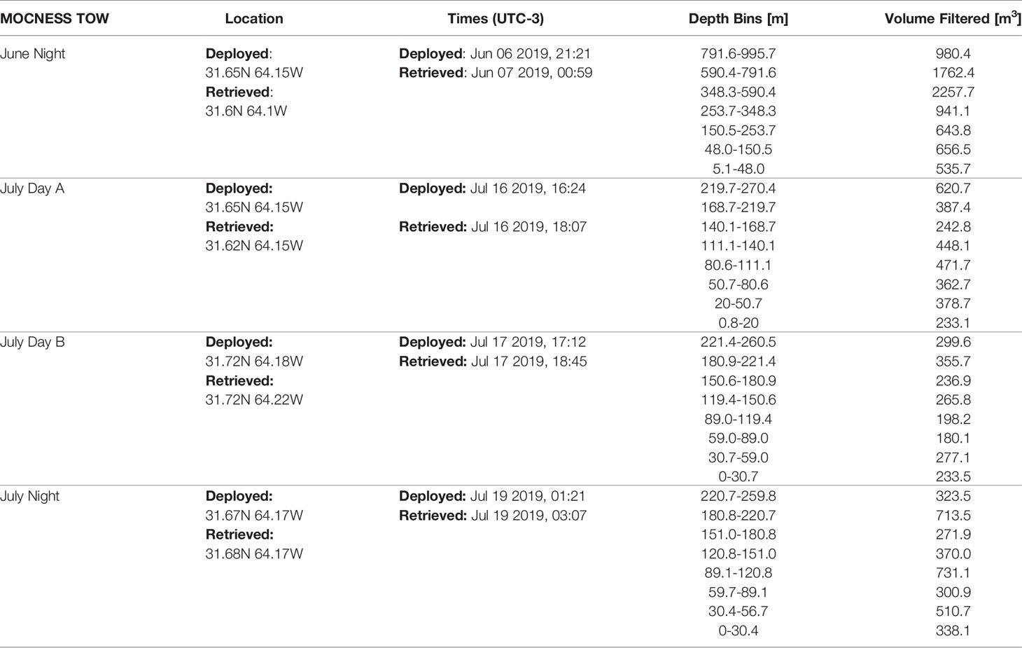
Table 2 MOCNESS metadata for the four tows.

2.2 Laboratory Processing of Net Samples

Fixed samples of plankton were transported back to the lab where they were measured using a ZooScan (Hydroptic; Gorsky et al., 2010). Samples collected from the June cruise (AE1912) were scanned at the University of South Carolina at 2400dpi. Samples from the July cruise (AE1917) were scanned at the Bermuda Institute of Oceanography at 4800dpi. To optimize segmentation (extracting vignettes of individual particle images from scanned samples), samples were size fractioned and split so that there were not too many particles in any given scan. Samples from the June cruise were split into two size fractions using a 1500μm sieve. Samples from the July cruise were split into three size fractions; all individual organisms larger than 2mm were removed by hand and imaged, then the samples were split using a 1000μm sieve. For all samples, the larger size fractions were split using a Motoda splitter (Motoda, 1959). All splits from the larger size fractions were scanned. For the smallest size fraction, it was important that there were not too many organisms in any single scan because this can impact the extraction of individuals. Samples from the June cruise were diluted while those from the July cruise were split to reduce concentrations in individual scan. For both approaches, enough scans were done so that there were at least 1500 objects scanned from each net. Scans were then processed using Zooprocess (Gorsky et al., 2010) to extract vignettes of individual objects. The default setting of the ZooScan extracts all objects larger than 300μm, a size much smaller than what is characterized by the UVP. For direct comparisons to the UVP dataset, the MOCNESS data was trimmed to only include plankton which were equal to or larger than the smallest identified plankton from UVP data. This size cutoff was determined to be 934μm.

2.3 Classification of Images and Morphology

The Ecotaxa web application was used to sort vignettes from both instruments (UVP and Zooscan) using a random forest classifier (Picheral et al., 2017; https://ecotaxa.obs-vlfr.fr/). All predicted identification were subsequently verified or reclassified by the same trained annotator. Generally, images collected by the UVP cannot be reliably classified to the same taxonomic resolution as images collected by the MOCNESS/ZooScan due to lower image resolution. As a result, many taxa were grouped into broad categories for comparison. Most notably, all Copepoda (Class: Hexanauplia, Subclass Copepoda) taxa were grouped to “copepod”, Decapods (Class: Malacostraca, Superorder: Eucardia, Order: Decapoda) and Euphausiids (Class: Malacostraca, Superorder: Eucardia, Order: Euphausiacea) were grouped to “shrimp-like crustaceans”, and ostracods (Class: Ostracoda) and cladocerans (Class: Brachiopoda, Subclass: Phyllopoda, Superorder: Diplostraca) were grouped to “Ostracod/Cladoceran”. Morphologically relevant metrics for each particle (major axis, minor axis, grey level, etc.) are computed in Zooprocess.

2.3.1 Management of ZooScan Vignettes With Multiple Organisms in a Single Vignette

Processing samples with the ZooScan requires manual separation of particles to facilitate the segmentation algorithm in zooprocess. However, it is inevitable that a few individual objects will not be separated during segmentation. Zooprocess allows for the post-processing of unseparated individuals. However, this can result in straight-lines and alter the accuracy of computed morphometrics. Additionally, there is a small portion of organisms which cannot be separated, even in post-processing if they are entangled or overlapping in a scan. To manage this challenge, we manually flagged all vignettes with multiple individuals during Ecotaxa classification. These vignettes were then re-examined, and individuals were counted after Ecotaxa classification. Because the morphometrics associated with these vignettes are inaccurate, we assigned each individual a set of randomly selected morphometric values from like taxa. Using this method assumes that the morphology of an organism does not influence the likelihood of it being caught in a multiple vignette, which for our dataset appeared to be a reliable assumption. This only affected 3% of our total MOCNESS data (Supplemental Information).

2.3.2 Assessing the Impact of Twice-Imaged Organisms in UVP Images

During validation of UVP vignettes, we noticed that there were cases where the same individual organism was imaged multiple times (Supplemental Figure 2). This can occur when the UVP is descending at a rate slower than the rate required to avoid overlap of images. It appears to be a concern primarily with larger, darker organisms. To assess the impact of multiple recordings of individuals, for all casts aboard AE1912, we sorted vignettes which clearly were multiple recordings into a distinct category. Estimates of those specific taxa’s density were then estimated for each profile in 20-m bins following two methods. In the first method, multiple-imaged organisms were treated as standard observations and counted, then divided by the total volume sampled in that 20-m bin. In the second method, multiple-imaged organisms had all but one vignette removed, then to account for this removal, the recorded volume in a 20-m bin was reduced to the maximum possible volume for non-overlapping UVP images in a 20-m stack (0.643m³).

2.4 Data Processing

To compare data collected from UVP casts to MOCNESS tows, UVP casts were categorized as either day or night for each month (Table 1). Sunrise and sunset times were calculated using the NOAA ESRL Solar Calculator (https://gml.noaa.gov/grad/solcalc/). To account for any potential diel vertical migration, casts which occurred within an hour before or after sunrise/sunset were marked as twilight and not included. There were no MOCNESS tows conducted near twilight hours.

First the instruments were compared on their scope of sampling to assess which taxa can be compared between the two devices. While the UVP was set to record all particles above 500 μm, larger sizes were required to reliably identify objects as living organisms. The smallest living organism recorded by the UVP was 0.934 mm. Because of this, MOCNESS-collected plankton which were smaller than 0.934 mm were excluded from all analyses. Then the relative contribution of different taxonomic groups were compared between the instruments. Finally, Annelids, Copepods, Chaetognaths, Shrimp-like crustaceans, and Ostracod/Cladocerans were selected for direct comparison.

2.4.1 UVP Cast Binning and Aggregating

UVP casts were binned into distinct depth bins in which concentration could be calculated. For depth specific bin comparison, the UVP bins were set to match the MOCNESS depth bins. However, a benefit of the UVP is the ability to resolve finer-scale patterns in mesozooplankton. Thus, for visualization and depth-integration, UVP bins were independently set. To select the independent bin size, depth integrated abundance was calculated for different taxa in individual UVP casts using trapezoidal integration across a range bin sizes. The smallest bin size which still yielded stable estimates was found to be 20-m (Supplemental Figure 4; Supplemental Information).

There were two methods utilized to aggregate the several UVP casts which correspond to a single MOCNESS tow. The first method is a pooled-cast approach. In this method, all similar casts are pooled into one representative profile. Then the concentration of observations (either counts or summed biomass) were calculated for each depth bin (Equation 1). This approach is common in UVP studies as it can increase the volume sampled in an individual depth bin.

Equation 1:

Pooled-cast calculation for a UVP depth bin concentration of i observations (counts or biomass) for all N casts in a depth bin.

The other method was an average-cast approach. This calculated concentration in a depth bin in each individual cast, then took the mean of all similar casts (Equation ). This approach allows for the characterization of mean and standard deviation between similar casts.

Equation 2.

Average-cast method for a UVP depth bin. The concentration of i observations summed across all N casts then divided by the number of casts.

2.5 Taxa-Specific Comparison of Density

To assess patterns of density throughout the water column, the concentrations of each comparable taxa were plotted using independent UVP bins with both pooled-cast and average-cast methods overlayed on MOCNESS data. Then, to quantify the difference in depth specific density estimates between the two sampling methods, linear regressions were conducted between the estimated concentration of each comparable taxa. For this analysis, the concentration of organisms was calculated in each depth-bin as determined by the MOCNESS tows. Regressions were done between pooled-cast UVP data versus MOCNESS data and average-cast UVP versus MOCNESS. For the average-cast approach, the mean concentration was used.

Then, the depth integrated abundance was calculated for all UVP and MOCNESS profiles. Due to the difference in sampling methodology, the June cruise was split into an epipelagic zone and mesopelagic zone. This provided two split integrations from data collected at the same location. Depth integration used trapezoidal integration with linear approximation between the mid-points of each depth bin (Supplemental Information; github.com/thealexbarth/EcotaxaTools). UVP casts used independent bin sizes for this integration. For the pooled-cast method, one integration was done over the whole pooled-cast. For the average-cast methods, integrations were done on each individual UVP cast, then the mean depth integrated abundance was found for similar casts. Paired Wilcox signed rank tests were used to compare depth integrated abundance between the different methods for each taxa.

2.6 Taxa-Specific Comparison of Biomass

For all comparable taxa, the volume of each individual vignette was calculated following assuming an ellipsoidal shape (Equation 3). This required the conversion of pixels to mm, which was a different conversion for each device (Supplemental Information).

Equation 3.

Biovolume estimation for an individual plankton vignette assuming an ellipsoidal shape.

Then, dry mass was calculated for each individual using biovolume to mass conversions described in Maas et al. (2021). Because the UVP does not facilitate high taxonomic specificity, we assigned all copepods the conversion factor for Calanoida, and all shrimp-like crustacean the conversion factor for Decapoda. Annelids were excluded from this analysis because there was not an available conversion factor. The biomass concentration (mg m^-3) was calculated for each depth bin by summing the biomass of all individuals of a given taxa then dividing by the total volume sampled in that depth bin. This was done using both the pooled-cash approach and average-cast approach for the UVP. Again, linear regressions were used to compare the direct calculations of biomass concentration between the MOCNESS and the two UVP approaches. Then the depth integrated biomass was calculated following the same steps as for the abundance. Paired Wilcox signed rank tests were used to compare depth integrated biomass between the different methods for each taxon.

All data were processed using R ver. 4.0 (R Core Team). Data were processed largely using the EcotaxaTools package (github.com/TheAlexBarth/EcotaxaTools). All data and code are available in Supplemental Information 1.

3 Results

3.1 Scope of Instruments

Images of the MOCNESS-collected plankton acquired by the ZooScan are generally much higher resolution than the in situ images acquired by the UVP (Figure 1). Although the UVP does acquire images which are capable of identifying several taxa in situ, the MOCNESS facilitates identification to a higher taxonomic resolution than the UVP. Notably, copepods sampled by the MOCNESS/ZooScan can be separated into at least the order level, and at times the family level. While some larger Calanoid copepods can easily be identified from UVP images, smaller copepods cannot be reliably identified to higher taxonomic resolution (Figure 1). From the MOCNESS tows, it appears that the majority of copepods sampled in this system are Calanoids or Cyclopoids, with a smaller percentage of Harpacticoids. The UVP can detect both decapods and euphausiids, although these cannot be reliably distinguished in most vignettes, so they were grouped to Eumalacostraca (referred to as shrimp-like crustacean). The MOCNESS/ZooScan images can be consistently distinguished as euphausiids or decapods, although for comparison to the UVP, we combined these as shrimp-like crustaceans. Additionally, the MOCNESS is able to sample meroplankton, larval forms, and fish (Figure 1). A few fish were sampled by the UVP, although these were often while in motion (Figure 1).

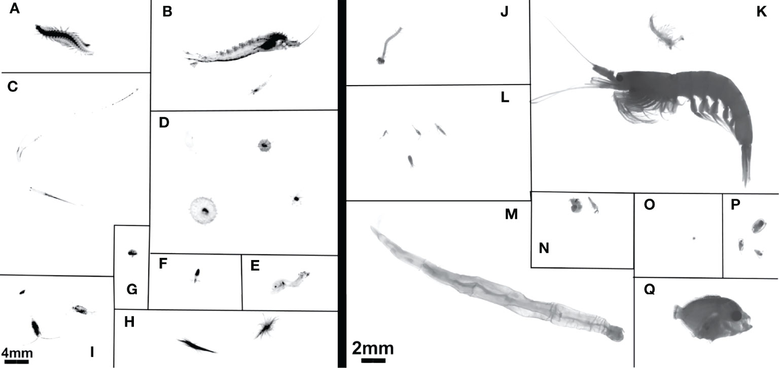
Figure 1 Example images from (A–I) the UVP and (J–Q) MOCNESS. UVP images have 4mm scale bar in bottom left. MOCNESS images use 2mm scale bar in bottom right. UVP images are (A) Annelida, (B) Shrimp-like Crustacea, (C) Chaetognatha, (D) Rhizaria, (E) Actinopterygii, (F) Mollusca, (G) Ostracoda, (H) Trichodesmium, (I) Copepoda. MOCNESS images are (J) Annelida, (K) Shrimp-like Crustacea, (L) Copepoda, (M) Chaetognatha, (N) Mollusca, (O) Acantharea, (P) Ostracoda, (Q) Actinopterygii.

Recording multiples of an individual did not have a clear effect on the UVP density estimates. After visually investigating the difference between taxon-specific density estimates for all June UVP casts when including multiple-recorded individuals and excluding them, we found no observable pattern (Supplemental Figure 3). This issue was most noticeable in select rhizaria and Trichodesmium images and inclusion of multiples would slightly increase density estimates. Alternatively, the exclusion method of multiple images also at times increased density estimates (Supplemental Figure 3). Thus, we determined it would be best to include multiples, particularly because the exclusion requires alteration of the volume sampled measurement, which can then decrease the accuracy of concentration estimate for all other taxa.

As expected, the MOCNESS sampled a much larger size range than the UVP. The ZooScan is set to record all individual particles larger than 300μm ESD while the UVP is set to record all individual particles larger than 500μm ESD. However, the images collected by the UVP could only be reliably identified for much larger particles. Thus, the smallest living organism collected by the UVP identified was 934μm. For comparison, all MOCNESS-collected plankton below this size were excluded. This exclusion removes a large portion of the plankton collected by the MOCNESS (Supplemental Figure 5). Notably, 91.2% and 96.7% of copepods and ostracods/cladocerans respectively, sampled by the MOCNESS were smaller than 934μm. For other MOCNESS-collected plankton, 30% of annelids were below this size cut-off while only 11% of chaetognaths and 6.98% of Shrimp-like crustaceans. With the size trimmed MOCNESS data, there was a considerable overlap with the UVP in the size distribution of all plankton (Figure 2). The median MOCNESS size was 1.87mm. The median UVP size was 1.56mm. For specific taxa, the MOCNESS generally sampled across sizes more evenly than the UVP, which had its size distributions more concentrated (Figure 2). There was a large size overlap for copepods although the MOCNESS median (1.51mm) was slightly larger than the UVP median (1.31mm) (Figure 2C; Supplemental Information). Interestingly, the MOCNESS seemingly sampled larger chaetognaths and shrimp-like crustaceans better than the UVP. The MOCNESS size distribution for those taxa had secondary peaks between 3-3.75mm, where there were very few UVP-imaged plankton at those sizes (Figures 2B, E). Alternatively, the UVP size distributions for annelids and ostracods/cladocerans were shifted upwards and had little overlap with the MOCNESS distributions (Figures 2C, F).

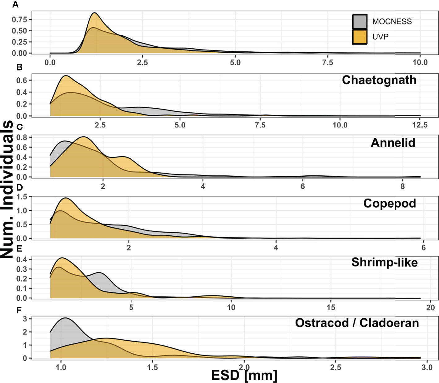
Figure 2 Size distribution compared between MOCNESS-collected plankton (excluding those smaller than 934μm) and UVP-imaged plankton for (A) All living organisms, (B) chaetognaths, (C) annelids, (D) copepods, (E) shrimp-like crustaceans, (F) ostracods/cladocerans. For all living organisms, those larger than 10mm ESD were excluded to allow for visualization. Notes that between each panel y and x axis differ.

Even with the size trimmed data, the MOCNESS tow recorded a much larger diversity of taxa than the UVP (Figure 3). Across all MOCNESS tows, copepods were proportionally the most abundant organisms, representing a third of all recorded organisms (Figure 3). The proportion of copepods observed by the UVP was slightly smaller, at 27% of all living organisms across all casts (Figure 3; Supplemental Information). Of all recorded particles from UVP casts, approximately 84.5% were detritus or unidentifiable particles. Among living organisms, Rhizaria and Trichodesmium made up 39.4% and 17.5% of all UVPs observations respectively. Interestingly, Trichodesmium abundance was greatly varied between the two cruises (Figure 3). The MOCNESS tows did not record any Trichodesmium while it did record a few rhizaria cells. Typically, rhizaria cells sampled by the MOCNESS were small acanthareans or foraminiferans. While both these taxa are sampled by the UVP, in situ vignettes collected by the UVP reveal a much larger diversity of Rhizaria, including many large phaeodarians and radiolarians. Mollusca, generally pteropods, were a sizeable portion of MOCNESS sampled organisms however they were not sampled adequately by the UVP (Figure 3). Organisms which were sampled by both instruments in sizeable numbers were copepods, shrimp-like crustaceans, chaetognaths, ostracods/cladocerans, and annelids. It should be noted that in UVP casts, shrimp-like crustacean and chaetognath proportions were roughly equivalent (3.2% and 3.4% respectively) (Figure 3). However, in MOCNESS samples, the chaetognath proportion was generally over double shrimp-like crustacean (Figure 3).

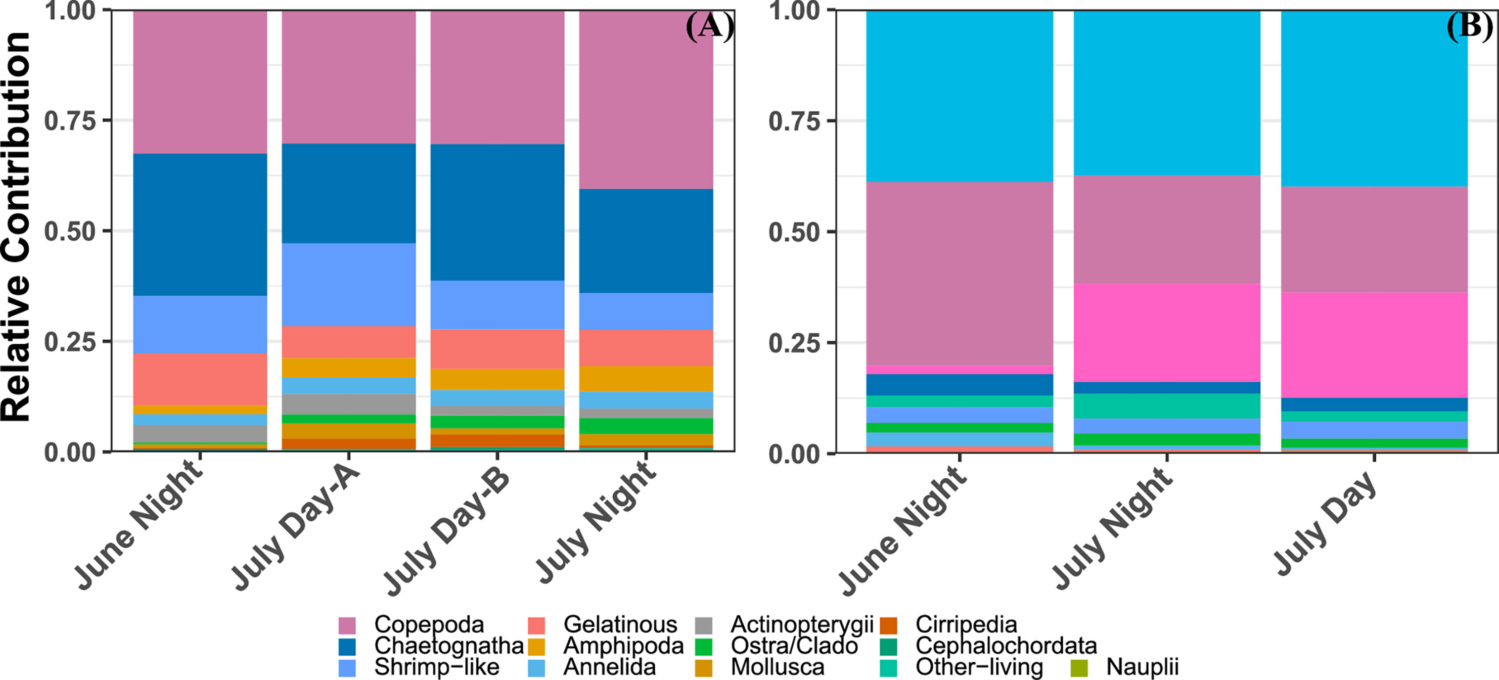
Figure 3 Relative contribution of different zooplankton groups to the total living abundance from each profile from (A) the MOCNESS/ZooScan plankton above the 934μm size cut-off and (B) the UVP.

3.2 Comparison of Density Estimates Between Sampling Methods

In general, the UVP had much lower estimates of abundance across all five investigated taxa (Figure 4 and Supplemental Figure 6). However, the average-cast approach revealed that there was large variation between individual casts. Generally, the pooled-cast approach and average cast approach led to the similar estimates. For taxa which had higher concentrations of individuals (copepods, chaetognaths, and shrimp-like crustaceans), the UVP was able to partially capture vertical patterns (Figures 4A–C). However, this result was inconsistent, particularly for chaetognaths and shrimp-like crustaceans for which the UVP had much more variation between casts and did not follow MOCNESS patterns. (Figures 4D–F). For the taxa with lower concentrations (ostracods/cladocerans and annelids), the UVP did not capture the vertical structure of those populations. Interestingly however, the UVP did detect both annelids and ostracods in regions of the water column where the MOCNESS did not (Figures 4G–I). Although variation in the average-cast approach for these taxa was very large.

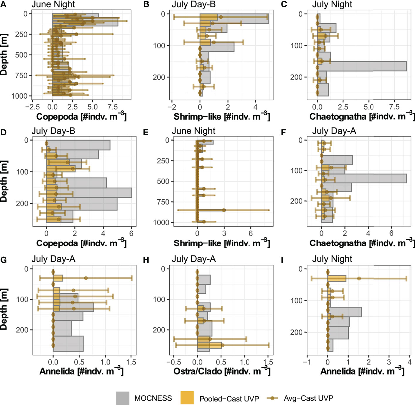
Figure 4 Selected profiles of taxa density estimates by the MOCNESS, pooled-cast UVP, and average-cast UVP calculations. Pooled-cast UVP is shown as bars while average-cast UVP is shown mean points with standard deviation. MOCNESS depth-bins are determined by net deployment while UVP bins are 20m Profiles are selected to show (A–C) cases where the vertical pattern of plankton shown by the MOCNESS is captured by the UVP, (D–F) cases where the UVP does not emulate the MOCNESS, and (G–I) cases of annelids and ostracod/cladocerans. (A) Copepod density estimates from June night. (B) Shrimp-like density estimates from July Day-B. (C) Chaetognath density estimates from July Night. (D) Copepod from July Day-B. (E) Shrimp-like density estimates from June night. (F) Chaetognath density estimates from July Day-A. (G) Annelid density estimates from July Day-A. (H) Ostracod/Cladoceran density estimates from July Day-A. (I) Annelid density estimates from July night. All profiles are available in Supplemental Figure 6.

UVP concentrations calculated in matching depth bins to the MOCNESS were analyzed with linear regressions to quantify if there was a predictable pattern of under/over sampling. For shrimp-like crustaceans, there was a significant relationship between the pooled-cast UVP estimates and MOCNESS estimates (b_{1 =} 0.073, p-value = 0.01, r² = 0.21) (Figure 5I) and a significant relationship between average-cast UVP estimates and MOCNESS estimates (b₁ = 0.094, p = 0.007, r² = 0.23) (Figure 5J). However, this relationship appears to be spurious as there is high heteroskedasticity around the regression line, with only a few, influential observations at higher concentrations. For all other taxa, no significant relationships were found between either the pooled-cast UVP or the average-cast UVP and the MOCNESS (Supporting Information). In general, UVP estimates fell below the 1:1 line with MOCNESS estimates (Figure 5). However, annelids and ostracods/cladocerans had more observations closer to the 1:1 line. Yet, for both those taxa, there were more observations where only one instrument measured any individuals, and the other did not (Figure 5).

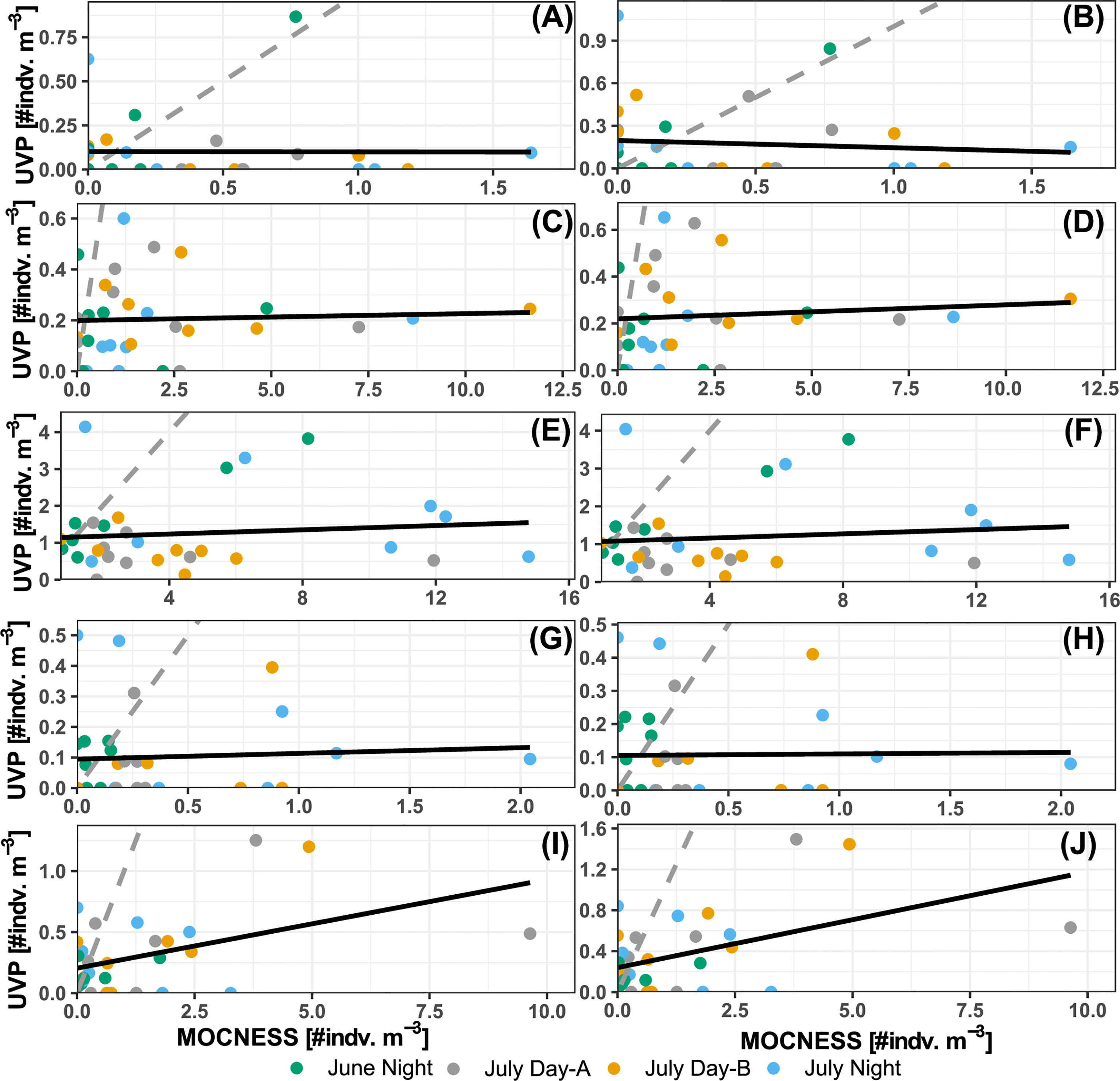
Figure 5 Comparison of MOCNESS density estimates and (A, C, E, G, I) pooled-cast UVP density. Comparison of MOCNESS density estimates and (B, D, F, H, J) average-cast UVP density estimates. Points show density estimates in matching depth bins for (A, B) Annelids, (C, D) chaetognaths, (E, F) copepods, (G, H) shrimp-like crustacean, and (I, J) ostracod/cladocerans. Points are colored by corresponding profile. Dotted line represents the 1:1 line between the two estimates. Solid line shows the line of best fit identified through least squares regression.

Once integrating abundance throughout the water column, the taxon-specific estimates were closer between the different methods. For all taxa, the MOCNESS depth integrated abundance was generally larger than the both the pooled-cast and average-cast UVP depth integrated abundances (Figure 6). However, this trend was not a statistically significant difference for any taxa (Paired Wilcox sign rank test, p > 0.05; Supporting Information). Interestingly, in the UVP integrated abundance estimates in the mesopelagic were much closer, and in cases, higher than the MOCNESS estimates (Figure 6). Additionally, it was found for all taxa that there was no significant differences between the pooled-cast and average-cast UVP approach (Paired Wilcox sign rank test, p>0.05; Supporting Information).

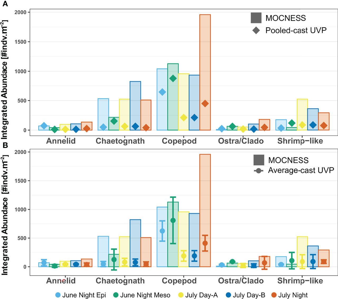
Figure 6 Depth integrated abundance for each specific taxon comparing MOCNESS estimates to (A) pooled-cast UVP and (B) average-cast UVP calculations. For average-cast calculations, error bars indicate standard deviation between depth integrated abundance of similar UVP profiles. Colors indicate the corresponding integrated profile/tow. Note that the June night tow was integrated as an epipelagic region (0-250) and a mesopelagic region (250-1000). There were no significant differences in integrated abundance for taxon-specific comparisons between the MOCNESS vs pooled-cast UVP; MOCNESS vs average-cast UVP; nor the pooled-cast vs average-cast calculation (Paired Wilcox sign rank test, p > 0.05).

3.3 Comparison of Biomass Calculation Between Sampling Methods

Biomass concentration (mg m^-3) was then estimated for annelids, chaetognaths, copepods, and shrimp-like crustaceans. Similar to the abundance profiles, the MOCNESS generally had larger biomass concentrations than both UVP methods in comparable areas of the water column (Figure 7). The biomass concentration for shrimp-like crustacean and chaetognaths were extremely variable between UVP casts (Figures 7B, C). There was no significant relationship of chaetognath biomass concentration estimates between the pooled-cast UVP and MOCNESS nor between the average-cast UVP and MOCNESS (Figures 8A, B; Supporting Information). However, there were significant relationships between both the UVP methods and the MOCNESS estimates for biomass concentrations of shrimp-like crustaceans, copepods, and ostracod/cladocerans (Figures 8C–H; Supporting Information). This finding is particularly surprising, given that there was not a meaningful relationship between the abundance estimates between the two devices. It is likely that the regression slopes between the UVP and MOCNESS are not meaningful despite their statistical significance.

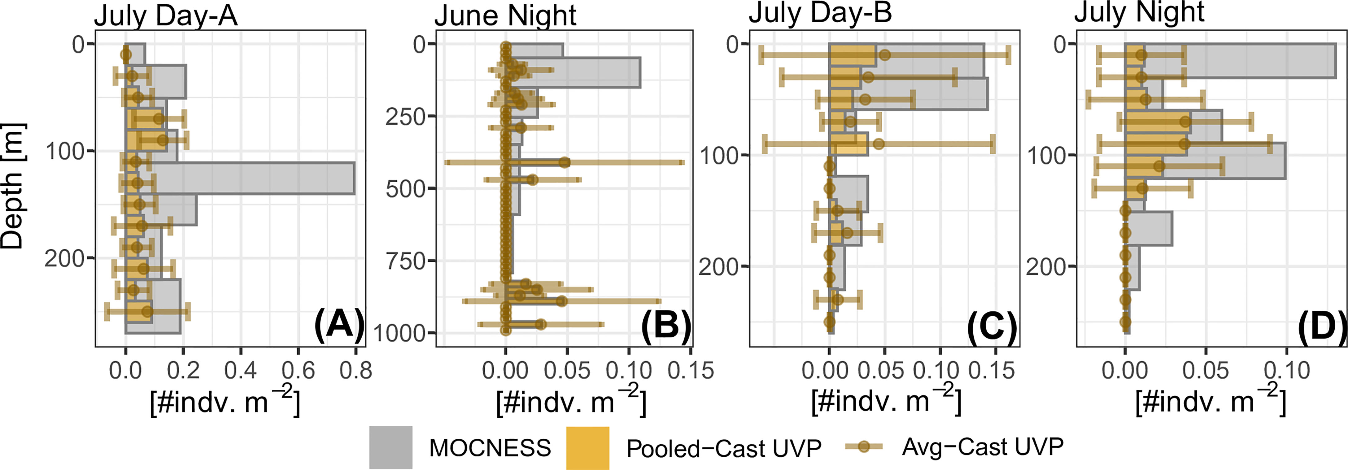
Figure 7 Select profiles of taxa biomass concentration calculated from MOCNESS, pooled-cast UVP approach, and average-cast UVP approach. Profiles are selected to show examples for (A) copepods, (B) chaetognaths, (C) shrimp-like crustaceans, and (D) ostracod/cladocerans. All profiles can be seen in Supplemental Figure 7.

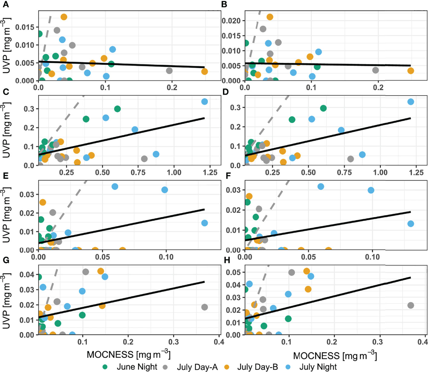
Figure 8 Comparison of biomass concentration estimates between MOCNESS to (A, C, E, G) pooled-cast UVP method and between MOCNESS to (B, D, F, H) average-cast UVP method. Taxon-specific regressions are for (A, B) chaetognaths, (C, D) copepods, (E, F) ostracods/cladocerans, and (G, H) shrimp-like crustaceans. Dotted grey line indicates 1:1 relationship while the solid grey line identifies the line of best fit determined by ordinary least squares regression.

Finally, depth integrated biomass concentration estimates calculated by the UVP methods were close, yet lower than those calculated by the MOCNESS (Figure 9). This trend was not significantly different for any of the taxa for both the pooled-cast versus MOCNESS nor the average-cast versus MOCNESS (Paired Wilcox signed-rank test, p-value > 0.05, Supporting Information). Additionally, there was no significant difference in depth integrated biomass concentration estimates between either of the UVP methods, for all taxa (Paired Wilcox signed-rank test, p-value > 0.05, Supporting Information).

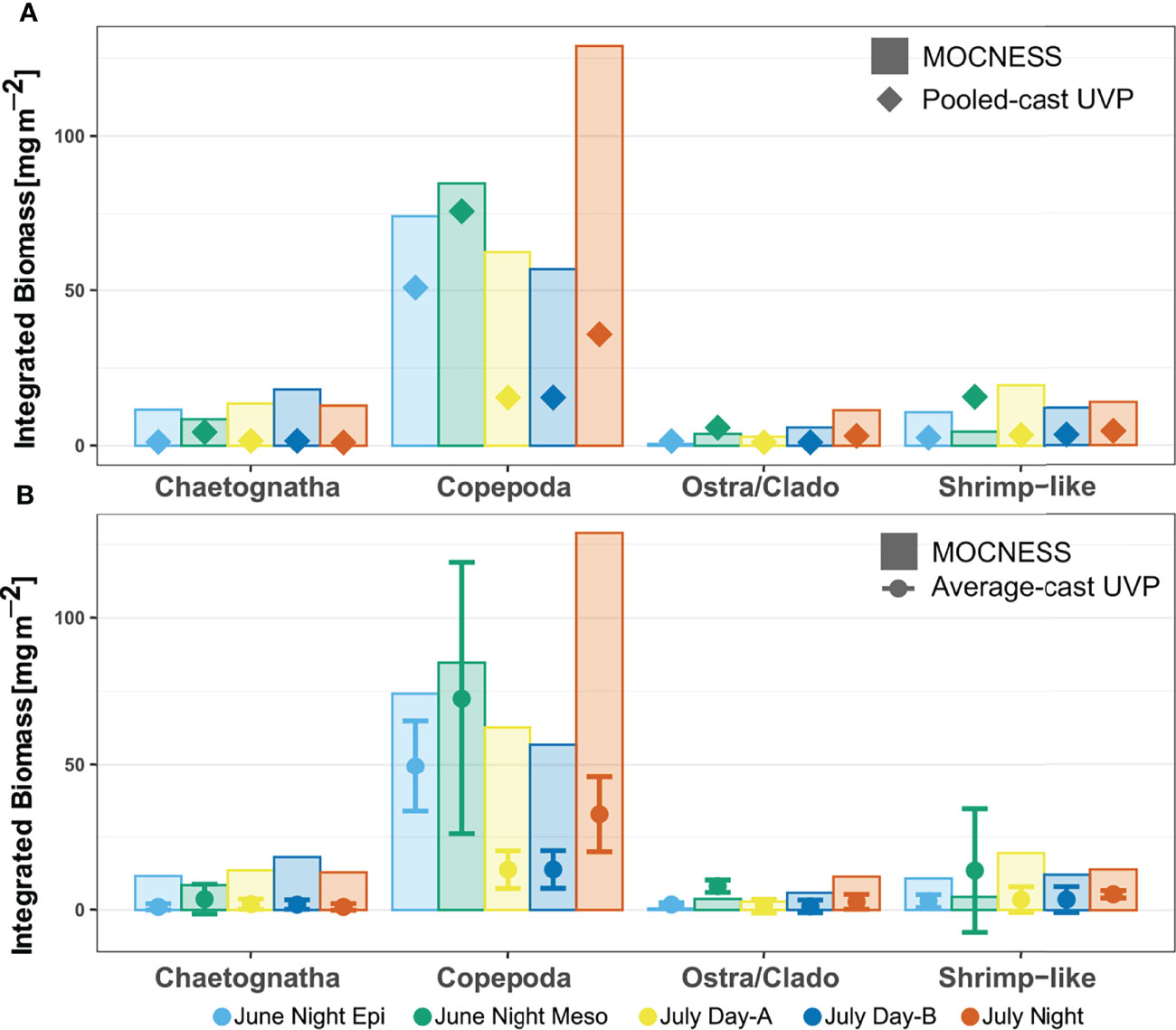
Figure 9 Depth integrated biomass for each specific taxon comparing estimates from MOCNESS to (A) pooled-cast UVP calculations and to (B) average-cast UVP calculations. Average-cast UVP calculations show standard deviation between similar UVP casts. There were no significant differences in the taxon-specific estimated depth integrated biomass between MOCNESS to pooled-cast UVP, MOCNESS to average-cast UVP, nor pooled-cast to average-cast UVP.

4 Discussion

4.1 Scope of Instruments

Generally, the MOCNESS/ZooScan produces higher quality images allowing for superior taxonomic resolution compared to the UVP. Use of the MOCNESS is necessary to sample a large portion of the copepod and ostracod community in the oligotrophic ocean which are not able to be sampled by the UVP due to their small size. Once looking at comparable size ranges however, the UVP and MOCNESS had copepods represent a similar proportion of the total sampled organisms. However, aside from copepods, the relative abundance of taxa varied between the devices. The, MOCNESS’s next largest categories of sampled plankton were chaetognaths and shrimp-like crustaceans. The UVP’s other common organisms by abundance were Rhizaria and Trichodesmium. Fragile taxa such as these are likely destroyed in the MOCNESS and formalin preservation process and thus under sampled by net-based methods. MOCNESS destruction or fragmentation of annelids could also explain why the UVP sampled a seemingly larger size distribution of that taxa. The effectiveness of the UVP for sampling such fragile taxa have been demonstrated in previous studies (Biard et al., 2016; Stukel et al., 2019). Additionally, while in the present study, all rhizaria taxa were grouped broadly, it is possible to use UVP images to categorize rhizaria into families (Figure 1; Biard et al., 2016). Interestingly, in our study we found rhizaria to be a higher proportion of all mesozooplankton by abundance compared to previous studies in the region (Biard et al., 2016), indicating that there is likely large variation in rhizaria abundance across some time scales.

The MOCNESS/ZooScan also sampled a much larger size range than the UVP did. This was an unsurprising finding given that the ZooScan can record particles above 300μm while the UVP is set to only save vignettes of particles larger than 500μm. However, the UVP vignettes at the smaller sizes (500μm – 1000μm) were too coarse to identify as living organisms. Additionally, another consideration for the size estimates of UVP organisms is that plankton can be oriented in any direction during imaging. Thus, if a plankter is positioned orthogonally to the UVP’s camera its true size might be underestimated. Additionally small plankton in such orientations might be difficult to identify. As a result, the smallest UVP-imaged particles identified to be a living organism were at least 934μm and for some taxa, they were over a millimeter. Forest et al. (2012) also observed that the UVP did not sample copepods well below a 1mm. In oligotrophic systems like the Sargasso Sea, there are a large portion of the zooplankton community which is not sampled by the UVP because they are smaller than 900μm (Supplemental Figure 5). Certainly, there is a portion of the particles recorded by the UVP which are truly living organisms, yet the images of them are too coarse to distinguish as living organisms. It is likely that the upward shift in the UVP ostracod size distribution was caused by the difficulty of distinguishing smaller ostracods and cladocerans from particles. While the particle data do not allow for taxon-specific density or biomass estimation, this information can be used to characterize communities based on particle size spectra (Sprules and Barth, 2016; Lombard et al., 2019).

While the majority of the taxa sampled by the MOCNESS were smaller than those sampled by the UVP, there were a few taxa which had larger size classes that the UVP did not sample either. This was most notable with the chaetognaths. A sizable portion of the chaetognaths measured by the MOCNESS were 3mm to 7.5mm ESD. The UVP hardly imaged any chaetognaths in this size range. It is likely that larger organisms are able to avoid the CTD-rosette. Many of the chaetognaths which were imaged by the UVP were actively in motion (Figure 1). Additionally, many fish and shrimp-like crustaceans measured by the UVP were also in motion. Other in situ imaging devices have documented krill showing an escape response when encountered with the device (Hoving et al., 2019). However, Hoving et al. (2019) used a white-light system. For imaging devices to minimize zooplankton response, the device must be designed specifically to reduce disturbance (Ohman et al., 2018). The UVP5 is equipped with red LED lights, intending to reduce escape response by zooplankton. The cause of plankton disturbance in this study is unclear. The UVP was positioned inside a large CTD rosette, thus it could have been the physical turbulence caused by the large frame initiating the escape response and not the light. Chaetognaths in particular have long been known to rely on tactile rather than visual cues to initiate movement (Horridge and Boulton 1967). Avoidance is also a challenge for net-based systems; however, our results indicate that avoidance is also a potential large issue for studying certain taxa with the UVP.

4.2 Density Estimates and Biomass Calculations

Generally, the UVP underestimated density across all compared taxa. For annelids and ostracods/cladocerans, there are likely too few organisms for the UVP to adequately sample. This is clearly observed in the depth profiles for these taxa which show small, infrequent peaks and high variation in the average-cast UVP profiles (Figure 4 and Supplemental Figure 5). The UVP sampling volume, even with pooled casts, is still too low to adequately sample these sparser zooplankton. Increasing the imaged volume is a critical step for in situ optical tools (Cowen and Guigand, 2008; Lombard et al., 2019). Chaetognath, shrimp-like crustaceans, and copepods were all well sampled by the UVP, however the density estimates were still much lower than the MOCNESS. Other studies have used a “relative index” for large copepods sampled by the UVP (Donoso et al., 2017), however our results did not support a clear relationship for estimates of any taxa from the UVP to the MOCNESS. A contributing factor to the under sampling of some of these organisms is likely the mobility of these plankton and their avoidance of the CTD rosette as it descends through the water column. Copepods are decently sampled by the UVP, yet because the UVP only sampled large copepods, it is missing a sizable portion of the oligotrophic copepod community. Large copepods are inherently less abundant and thus require larger volumes filtered to adequately study. Our study did find a reliable relationship between UVP and MOCNESS estimates of biomass concentration for three of the four investigated taxa. However, because we know the UVP is estimating a different number of organisms than the MOCNESS, the biomass concentrations are likely faulty. This indicates that existing biovolume to dry mass relationships for net collected plankton may not be reliable for in situ imaged organisms.

Depth integration for both abundance and biomass concentration led to UVP estimates more similar to those of MOCNESS estimates. While estimates in matching depth bins were not similar, the similarity of depth integrated estimates can be explained by a few possibilities. First, depth integration effectively increases the volume filtered by combining several depth bins. Secondly, plankton are patchily distributed throughout the water column so populations of plankton may be a few meters deeper or shallower between nearby profiles. Finally, although our study did not find a significant difference in depth integrated estimates between MOCNESS and either UVP method, this could be a result of the low statistical power from the small sample size. There was a notable trend of lower UVP estimates in paired MOCNESS integrations.

4.3 Conclusion and Recommendations for In Situ Imaging

It is clear that the UVP under samples many categories of zooplankton compared to a MOCNESS. In more eutrophic systems, or areas where average body sizes are larger, the in situ imaging like will be more effective at estimating zooplankton abundance (Forest et al., 2012; Vilgrain et al., 2021). The mobility and escape response of zooplankton also need to be considered when attempting to characterize large zooplankton populations. In situ imaging studies should consider both the light and turbulence disruption caused by the sampling device.

This study identifies several methodological considerations for in situ imaging studies. Previous UVP studies have pooled similar casts, however this study shows that there is no significant improvement to pool casts rather than average them. We argue that averaging casts provides more information because the variation between casts is clearly represented. While some variation between casts may be due to the small sampling volume, patchiness can also be characterized for more abundant taxa. Selection of depth bin width to study plankton is also an important consideration. While increasing bin width does increase the volume sampled in a depth region, it sacrifices ecologically relevant information about plankton distributions. However, using too small of bin sizes can be misrepresentative. We encourage authors using in situ imaging tools to investigate the smallest reliable bin size to use in their systems (Supplemental Figure 4). Finally in our system, estimates of density and biomass were not affected by multiple individuals being imaged twice. However, this finding may not hold true in other systems or if the rate of descent for the UVP is decreased.

Data Availability Statement

The original contributions presented in the study are included in the article/Supplementary Materials. Further inquiries can be directed to the corresponding author.

Author Contributions

JS contributed to the design of study and deployment of instruments. AB processed lab samples and managed data and data analysis. JS and AB contributed to the writing and revision of the manuscript.

Funding

Funding for this data collection was provided by Simons’s Foundation International’s as part of BIOS-SCOPE to L.B.B. and A.E.M. Ship time was supported by the Bermuda Atlantic Time Series Study via the OCE grant #1756105 and NSF OCE grant #1756312.

Conflict of Interest

The authors declare that the research was conducted in the absence of any commercial or financial relationships that could be construed as a potential conflict of interest.

Publisher’s Note

All claims expressed in this article are solely those of the authors and do not necessarily represent those of their affiliated organizations, or those of the publisher, the editors and the reviewers. Any product that may be evaluated in this article, or claim that may be made by its manufacturer, is not guaranteed or endorsed by the publisher.

Acknowledgments

We thank Rod Johnson, the BATS technicians, and BATS program for facilitating data collection and assisting in UVP piloting. The R/V Atlantic Explorer staff and crew were instrumental in data collection. Ryan Rykaczewski helped the set-up of the UVP and with data collection. Leo Blanco-Bercial, Amy Maas, and Hannah Gossner assisted in zooscanning of MOCNESS samples and guidance on this project. The content of this manuscript was greatly improved through peer-reviewers’ thoughtful comments.

Supplementary Material

The Supplementary Material for this article can be found online at: https://www.frontiersin.org/articles/10.3389/fmars.2022.898057/full#supplementary-material

All data and code can be accessed at https://github.com/TheAlexBarth/Oligotrophic_in-situ_net_comparison

References

Biard T., Stemmann L., Picheral M., Mayot N., Vandromme P.. (2016). In Situ Imaging Reveals the Biomass of Giant Protists in the Global Ocean. Nature 532, 504–507. doi: 10.1038/nature17652
Christiansen S., Hoving H.-J., Schütte F., Hauss H., Karstensen J., Kortzinger A., et al. (2018). Particular Matter Flux Interception in Oceanic Mesoscale Eddies by the Polychaete Poeobius Sp. Limnol. Oceanogr. 63, 2093–2109. doi: 10.1002/lno.10926
Cowen R. K., Guigand C. M. (2008). In Situ Ichthyoplankton Imaging System (ISIIS): System Design and Preliminary Results. Limnol. Oceangr.: Methods 6, 126–132. doi: 10.4319/lom.2008.6.126
Davis C. S., Gallage S. M., Berman M. S., Haury L. R., Strickler J. R. (1992). The Video Plankton Recorder (VPR): Design and Initial Results. Arch. Hydrobiol. Beih. Ergebn. Limnol. 36, 1651–1653.
Donoso K., Carlotti F., Pagano M., Hunt B. P. V., Escribano R., Berline L. (2017). Zooplankton Community Response to the Winter 013 Deep Convection Process in the NW Mediterranean Sea. J. Geophys. Res.: Ocean. 122, 2319–2338. doi: 10.1002/2016JC012176
Durrieu de Madron X., Ramondenc S., Berline L., Houpret L., Bosse A., Martini S., et al. (2017). Deep Sediment Resuspension and Thick Nepheloid Layer Generation by Open-Ocean Convection. J. Geophys. Res.: Ocean. 122, 2291–2318. doi: 10.1002/2016JC012062
Forest A., Babin M., Stemmann L., Picheral M., Sampie M., Fortier L., et al. (2013). Ecosystem Function and Particle Flux Dynamics Across the Mackenzie Shelf (Beaufort Sea, Artic Ocean): An Integrative Analysis of Spatial Variability and Biophysical Forcings. Biogeosciences 10 (5), 2833–2866. doi: 10.5194/bg-10-2833-2013
Forest A., Stemmann L., Picheral M., Burdorf L., Robert D., Fortier L., et al. (2012). Size Distribution of Particles and Zooplankton Across the Shelf-Basin System in Southeast Beaufort Sea: Combined Results From an Underwater Vision Profiler and Vertical Net Tows. Biogeosciences 9 (4), 1301–1320. doi: 10.5194/bg-9-1301-2012
Gorsky G., Ohman M. D., Picheral M., Gasparini S., Stemmann L., Romagnan J.-B., et al. (2010). Digital Zooplankton Image Analysis Using the ZooScan Integrated System. J. Plankton. Res. 322, 285–303. doi: 10.1093/plankt/fbp124
Guidi L., Calil P. H. R., Duhamel S., Bjorkman K. M., Doney S. C., Jackson G. A., et al. (2012). Does Eddy-Eddy Interaction Control Surface Phytoplankton Distribution and Carbon Export in the North Pacific Subtropical Gyre? J. Geophys. Res.: Biogeosci. 117, G02024. doi: 10.1029/2012JG001984
Hauss H., Christiansen S., Schütte F., Kiko R., Lima M. E., Rodrigues E., et al. (2016). Dead Zone or Oasis Iin the Open Ocean? Zooplankton Distribution and Migration in Low-Oxygen Modewater Eddies. Biogeosciences 13 (6), 1977–1989. doi: 10.5194/bg-13-1997-2016
Herman A. W., Beanlands B., Phillips E. F. (2004). The Next Generation of Optical Plankton Counter: The Laser-OPC. J. Plankton. Res. 10 (26), 1135–1145. doi: 10.1093/plankt/fbh095
Holliday D. V., Donaghay P. L., Greenlay C. F., McGehee D. E., McManus M. M., Sullivan J. M., et al. (2003). Advances in Defining Fine- and Micro-Scale Pattern in Marine Plankton. Aquat. Liv. Resour. 16 (3), 131–136. doi: 10.1016/S0990-7440(03)00023-8
Horridge G. A., Boulton P. S. (1967) Prey Detection by Chaetognatha via Vibration Sense. Proc. Roy. Soc B. 168, 413–419. doi: 10.1098/rspb.1967.0072
Hoving H.-J., Christianesn S., Fabrizius E., Hauss H., Kiko R., Linke P., et al. (2019). The Pelagic In Situ Observation System (PELAGIOS) to Reveal Biodiversity, Behavior, and Ecology of Elusive Oceanic Fauna. Ocean. Sci. 15, 1327–1340. doi: 10.5194/os-15-1327-2019
Hoving H.-J., Neitzel P., Hauss H., Christiansen S., Kiko R., Robison B. H., et al. (2020). In SituObservations Show Vertical Community Structure of Pelagic Fauna in the Eastern Tropical North Atlantic Off Cape Verde. Sci. Rep. 10, 10.21798. doi: 10.1038/s41598-020-780255-9
Jouandet M.-P., Jackson G. A., Carlotti F., Picheral M., Stemmann L., Blain S. (2014). Rapid Formation of Large Aggregates During the Spring Bloom of Kerguelen Island: Observations and Model Comparisons. Biogeosciences 11, 4393–4406. doi: 10.5194/bg-11-4393-2014
Kiorboe T. (2011). What Makes Pelagic Copepods So Successful? J. Plank. Res. 33(5): 677–685. doi: doi: 10.1093/plankt/fbq159
Kiørboe T., Visser A., Andersen K. H. (2018). A Trait-Based Approach to Ocean Ecology. ICES. J. Mar. Sci. 75, 1849–1863. doi: 10.1111/j.1365-2427.2009.02298.x
Kiko R., Biastoch A., Brandt P., Cravatte S., Hauss H., Hummels R., et al. (2017). Biological and Physical Influences on Marine Snowfall at the Equator. Nat. Geosci. 10 (11), 852–858. doi: 10.1038/NGEO3042
Litchman E., Ohman M. D., Kiørboe T. (2013). Trait-Based Approaches to Zooplankton Communities. J. Plankton. Res. 35 (3), 473–484. doi: 10.1093/plankt/fbt019
Lombard F., Boss E., Waite A.M., Vogt M., Uitz J.. (2019). Globally Consistent Quantitative Observations of Planktonic Ecosystems. Front. Mar. Sci. 6: 196. doi: 10.3389/fmars.2019.00196
Maas A. E., Gossner H., Smith M. J., Blanco-Bercial L. (2021). Use of Optical Imaging Datasets to Assess Biogeochemical Contributions of the Mesozooplankton. J. Plank. Res. 43 (3), 475–491. doi: 10.1093/plankt/fbab037
Martin P., van der Loeff M. R., Cassar N., Vandromme P., d’Ovidio F., Stemmann L., et al. (2013). Iron Fertilization Enhanced Net Community Production But Not Downward Particle Flux During the Southern Ocean Iron Fertilization Experiment LOHAFEX. Global Biogeochem. Cycles. 27, 871–881. doi: 10.1002/gbc.20077
Miquel J.-C., Gasser B., Martin J., Marec C., Babin M., Fortier L., et al. (2015). Downward Particle Flux and Carbon Export in the Beaufort Sea, Artic Ocean; the Role of Zooplankton. Biogeosciences 12, 5103–5117. doi: 10.5194/bg-12-5103-2015
Motoda S. (1959). Devices of Simple Plankton Apparatus. Memoirs of the Faculty of Fisheries Hokkaido University. 7(1-2): 73–94
Nayak A. R., Malkiel D., McFarland M. N., Twardowski M. S., Sullivan J. M. (2021). A Review of Holography in the Aquatic Sciences: In Situ Characterization of Particles, Plankton, and Small Scale Biophysical Interactions. Front. Mar. Sci. 7. doi: 10.3389/fmars.2020.572147
Ohman M. D. (2019). A Sea of Tentacles: Optically Discernible Traits Resolved From Planktonic Organisms in Situ. ICES. J. Mar. Sci. 76 (7), 1959–1972. doi: 10.1093/icesjms/fsz184
Ohman M. D., Davis R. E., Sherman J. T., Grindley K. R., Whitmore B. M., Nickels C. F., et al. (2018). Zooglider: An Autonomous Vehicle for Optical and Acoustic Sensing of Zooplankton. Limnol. Oceangr.: Methods 17), 69–86. doi: 10.1002/lom3.10301
Orenstein E., Ayata S.-D., Maps F., Biard T., Becker E., Benedetti F., et al. (2021). Machine Learning Techniques to Characterize Functional Traits of Plankton From Image Data. HAL Open Sci. hal-03482282.
Orenstein E. C., Ratelle D., Briseño-Avena C., Carter M. L., Franks P. J. S., Jaffe J. S., et al. (2020). The Scripps Plankton Camera System: A Framework and Platform for in Situ Microscopy. Limnol. Oceanogr.: Methods 18, 681–695. doi: 10.1002/lom3.10394
Picheral. M., Catalano C., Brousseau D., Claustre H., Coppola L.. (2022). The Underwater Vision Profiler 6: An Imaging Sensor of Particle Size Spectra and Plankton, for Autonomous and Cabled Platforms. Limnol. Oceanogr.: Methods 20: 114–129. doi: 10.1002/lom3.10475
Picheral M., Catalano C., Brousseau D., Claustre H., Coppola L., Leymarie E., et al. (2021). The Underwater Vision Profiler 6: An Imaging Sensor of Particle Size Spectra and Plankton, for Autonomous and Cabled Platforms. Limnol. Oceangr.: Methods 20), 1775–1778. doi: 10.1002/lom3.10475
Picheral M., Colin S., Irrison J.-O. (2017) EcoTaxa, a Tool for the Taxonomic Classification of Images. Available at: http://ecotaxa.obs-vlfr.frhttp://ecopart.obs-vlfr.fr.
Picheral M., Guidi L., Stemmann L., Karl D. M., Ghizlaine I., Gorsky G. (2010). The Underwater Vision Profiler 5: An Advanced Instrument for High Spatial Resolution Studies of Particle Size Spectra and Zooplankton. Limnol. Oceanogr.: Methods 8, 462–473. doi: 10.4319/lom.2010.8.462
Puig P., de Madron X. D., Salat J., Schroeder K., Martin J., Karageorgis P., et al. (2013). Thick Bottom Nepheloid Layers in the Western Mediterranean Generated by Deep Dense Shelf Water Cascading. Prog. Oceanogr. 111, 1–23. doi: 10.1016/j.pocean.2012.10.003
Sandel V., Kiko R., Brandt P., Dengler M., Stemmann L., Vandromme P., et al. (2015). Nitrogen Fuelling of the Pelagic Food Web of the Tropical Atlantic. PLoS-One 10 (6), e0131258. doi: 10.1371/journal.pone.0131258
Schulz J., Barz K., Ludtke A., Zielinski O., Mengedoht D., Hirche H.-J. (2010). Imaging of Plankton Specimens With the Lightframe on-Sight Keyspecies Investigation (LOKI) System. J. Euro. Opt. Soc 5, 100175. doi: 10.2971/jeos.2010.10017s
Severin T., Kessouri F., Rembauville M., Sanchez-Perez E. D., Oriol L., Caparros J., et al. (2017). Open-Ocean Convection Process: A Driver of the Winter Nutrient Supply and the Spring Phytoplankton Distribution in the Northwestern Mediterranean Sea. J. Geophys. Res.: Ocean. 122, 4587–4601. doi: 10.1002/2016JC012664
Sprules W. G., Barth L. E. (2016). Surfing the Biomass Size Spectrum: Some Remarks on History, Theory, and Application. C. J. Fish. Aquati. Sci. 73, 477–495. doi: 10.1139/cjfas-2015-0115
Steinberg D. K., Carlson C. A., Bates N. R., Johnson R. J., Michaels A. F., Knap A. H. (2001). Overview of the US JGOFS Bermuda Atlantic Time-Series Study (BATS): A Decade-Scale Look at Ocean Biology and Biogeochemistry. Deep-sea. Res. II. 48, 1405–1447. doi: 10.1016/S0967-0645(00)00148-X
Steinberg D.K., Landry M.R. (2017). Zooplankton and the Ocean Carbon Cycle. Annu. Rev. Mar. Sci. 9: 413–444. doi: 10.1146/annurev-marine-010814-015924
Stukel M. R., Ohman M. D., Kelley T. B., Biard T. (2019). Feeding and Flux-Feeding Zooplankton as Gatekeepers of Particle Flux Into the Mesopelagic Ocean in the Northeast Pacific. Front. Mar. Sci. 6. doi: 10.3389/fmars.2019.00397
Thomsen S., Karstensen J., Kiko R., Krahmann G., Dengler M., Engel A. (2019). Remote and Local Drivers of Oxygen and Nitrate Variability in the Shallow Oxygen Minimum Zone Off Mauritania in June 2014. Biogeosci. Disc. 16, 979–998. doi: 10.5194/bg-16-979-2019
Turner J. S., Pretty J. L., McDonnell A. M. P. (2017). Marine Particles in the Gulf of Alaska Shelf System: Spatial Patterns and Size Distributions From in Situ Optics. Continent. Shelf. Res. 145, 13–20. doi: 10.1016/j.csr.2017.07.002
Vilgrain L., Maps F., Picheral M., Babin M., Aubrey C., Irrison J.-O., et al. (2021). Trait-Based Approach Using in Situ Copepod Images Reveals Contrasting Ecological Patterns Across an Artic Ice Melt Zone. Limnol. Oceangr. 9999, 1–13. doi: 10.1002/lno.11672
Waite A. M., Stemmann L., Guidi L., Calil P. H. R., Hogg A. M. C., Feng M., et al. (2016). The Wineglass Effect Shapes Particle Export to the Deep Ocean in Mesoscale Eddies. Geophys. Res. Let. 43, 9791–9800. doi: 10.1002/2015GL066463
Wiebe P. H., Benfield M. C. (2003). From the Hensen Net Toward Four-Dimensional Biological Oceanography. Prog. Oceanog. 56 (1), 7–136. doi: 10.1016/S0079-6611(02)00140-4
Wiebe P. H., Burt K. H., Boyd S. H., Morton A. W. (1976). A Multiple Opening/Closing Net and Environmental Sensing System for Sampling Zooplankton. J. Mar. Res., 34 (3), 1822–1824.
Keywords: in situ, plankton, oceanography, Sargasso Sea, sampling, ocean optics, copepod
Citation: Barth A and Stone J (2022) Comparison of an In Situ Imaging Device and Net-Based Method to Study Mesozooplankton Communities in an Oligotrophic System. Front. Mar. Sci. 9:898057. doi: 10.3389/fmars.2022.898057
Received: 16 March 2022; Accepted: 23 May 2022;
Published: 21 June 2022.
Edited by:
Elaine Fileman, Plymouth Marine Laboratory, United KingdomReviewed by:
Akash R. Sastri, Institute of Ocean Sciences, CanadaHelena Hauss, GEOMAR Helmholtz Center for Ocean Research Kiel, Germany
Copyright © 2022 Barth and Stone. This is an open-access article distributed under the terms of the Creative Commons Attribution License (CC BY). The use, distribution or reproduction in other forums is permitted, provided the original author(s) and the copyright owner(s) are credited and that the original publication in this journal is cited, in accordance with accepted academic practice. No use, distribution or reproduction is permitted which does not comply with these terms.
*Correspondence: Alexander Barth, AB93@email.sc.edu