Long-term mean circulation in the Japan Sea as reproduced by multiple eddy-resolving ocean circulation models

1. Introduction

Knowledge of long-term variations in heat, matter, and salt transport by highly variable ocean currents is essential to understanding the ocean climate of a semi-closed marginal sea. The Japan Sea is one of the largest marginal seas in the Northwest Pacific with a mean depth of 1,750 m, which is divided by the seamounts into three large basins: the Japan Basin, the Yamato Basin, and the Ulleung Basin (Figure 1). Recent studies have revealed a series of anomalous ocean environment changes occurring in the Japan Sea that are potentially related to the global warming trend. The sea surface temperature (SST) averaged over the Japan Sea has risen by 1.3°C–1.7°C during the last century (Kida et al., 2020). A long-term ocean acidification trend has been detected along the Japan coast (Ishida et al., 2021). Shipboard measurements also indicate a rapid freshening trend of the Japan Sea Intermediate Water and a decreasing trend of dissolved oxygen in bottom water of Japan Sea. All the above phenomena are significantly influenced by the ocean current, which exists in the form of a northeastward Japan Sea Throughflow (JSTF) due to the semi-closed topography in the Japan Sea and exhibits an interannual intensification trend similar to that of SST and sea surface height (SSH) (Kida et al., 2020). Therefore, it is of great importance to study the long-term variability of Japan Sea circulation patterns and predict its future, developing trend under the global warming background, which is mainly achieved by using numerical tools and high-quality reanalysis data.

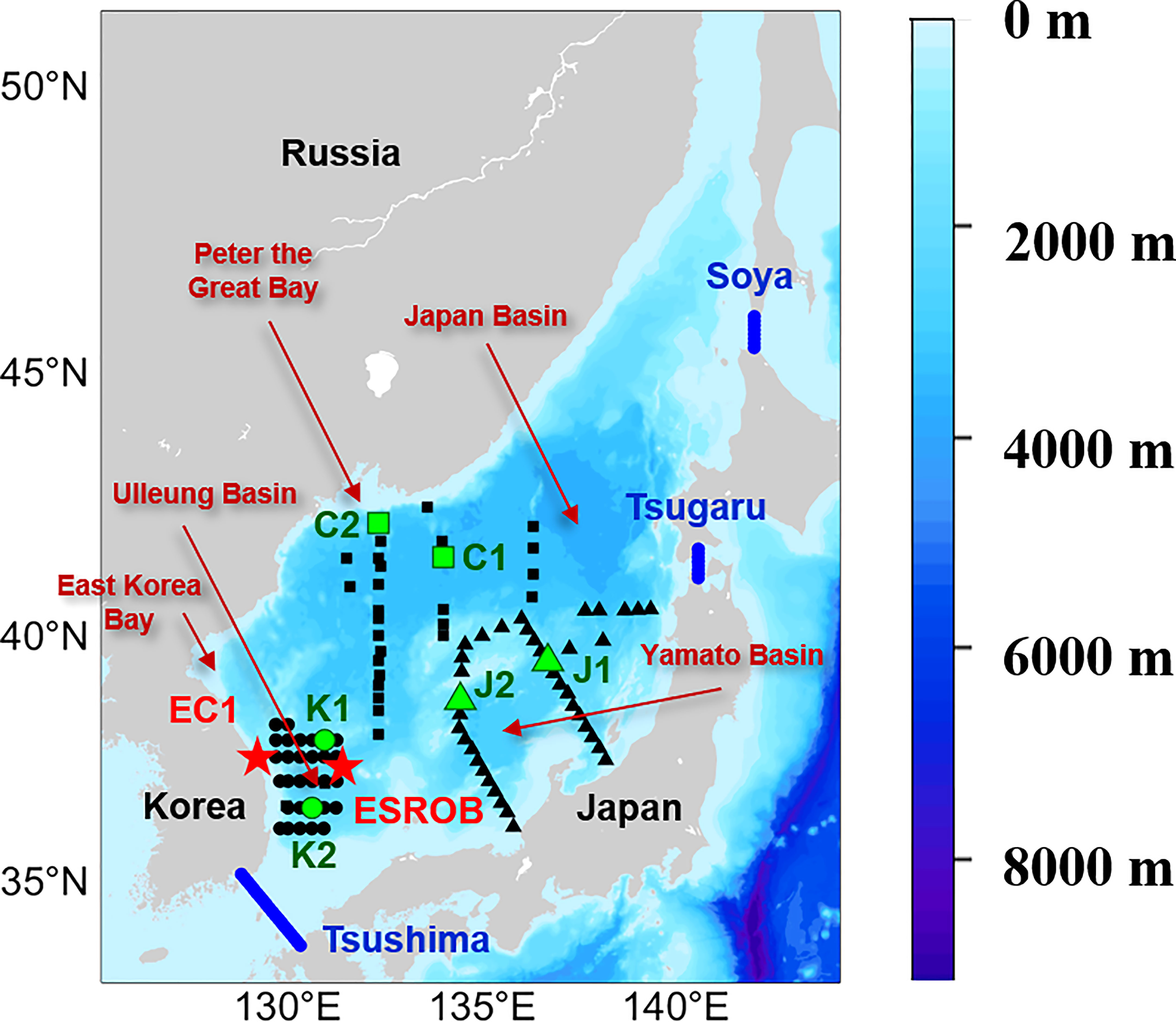
Figure 1 Locations of the used monitoring stations for the assessment of temperature and salinity (green marks) and current velocities (red pentagons) as well as the analyzed transects in three major straits (blue lines). Black marks denote hydrographic stations with more than 36 months of observation data. Round, square, and triangle circles denote KODC stations, CREAMS/EAST-I cruise stations, and JMA cruise stations, respectively. The background blue shading shows the bathymetry (m) from ETOPO1. See text for further information.

Because in situ measurements of JSTF are scarce in space and time, numerical modeling has become a necessary tool for studying the dynamics of ocean circulation in the Japan Sea. The first diagnostic model of horizontal circulation in the Japan Sea is based on a simple geostrophic balance applied by Yi (1966), which is the first attempt to estimate the mean values and seasonal variability of volume transport into the Japan Sea by using dynamic calculation. With the help of three-dimensional (3D) models on the basis of linear barotropic equations, Minato and Kimura (1980) and Ohshima (1987) investigated the driving mechanism of inflow through the Tsushima Strait and outflow through the Soya Strait. By establishing a barotropic model with shallow water equations, Ohshima (1994) forced the diagnostic model by using observed sea level difference across the strait and found that the geopotential anomaly between subtropical and subpolar gyres serves as the primary driver of the mean horizontal circulation in the Japan Sea. Despite the absence of atmospheric forcing in the models, their simple modeling experiments still obtained reasonable mean volume transport and vertical current profiles that are highly consistent with in situ measurements. In addition, with diagnostic models, Sekine (1986) evaluated the influence of wind-driven circulation on the branching of the Tsushima Warm Current and found that the winter monsoon critically determines the intensity of boundary currents in the Japan Sea. A similar conclusion was drawn from Spall (2002), where sensitivity experiments indicate that wind stress critically determines the formation of eastern boundary current in the Japan Sea, whereas the buoyancy forcing is primarily responsible for its maintenance.

Further modeling studies of the JSTF variability and dynamics are primarily based numerical models rather than analytical models. Kim and Yoon (1999) simulated the separation point of the East Korea Warm Current (EKWC) using Modular Ocean Model (MOM) with an isopycnal mixing scheme forced by the observed heat flux and wind stress data. Using Research Institute for Applied Mechanics Ocean Model (RIAMOM) with the boundary conditions from ADCP, Kawamura et al. (2009) well reproduced the branch structure of JSTF and the variations of sea level along the Japan coast without any data assimilation. Numerical experiments of Park et al. (2013) and Kim et al. (2020) revealed that the surface heat flux has significant influence on the mean upper ocean circulation patterns in the Japan Sea by affecting the thickness of mixing layer.

Lagrangian passive tracer is a useful tool to trace the origin and paths of large ocean current systems, which has been involved into the 3D regional models by Stepanov et al. (2020) in the middle Japan Sea and by Prants et al. (2022) and Fayman et al. (2019) in the Peter the Great Bay. Stepanov et al. (2020) explained the clustering phenomena of floating tracer in the middle Japan Sea by identifying a mesoscale ocean current field with various eddy structures. Prants et al. (2022) tracked the formation and deep convection of dense shelf water in winter by using Lagrangian maps in the Regional Ocean Modeling System (ROMS). They found that the modeling results may be affected by the atmospheric forcing, the water exchange in the strait, and the sea ice formation near the northern coast. In addition, by the Lagrangian experiments of ROMS, Fayman et al. (2019) confirmed the existence of mesoscale eddies near the Ussuri Bay and its specific function to carry dense water masses in Japan Sea.

Because of the narrow width of strait throughflow and boundary currents, dynamic studies on JSTF increasingly rely on eddy-resolving models. With the advances of supercomputing power, a large number of high-resolution numerical experiments on JSTF have appeared in recent studies. Examples include the topography experiment in Finite Volume Coastal Ocean Model by Han et al. (2018), the heat sensitivity experiment in RIAMOM by Kim et al. (2020) and Hirose et al. (2021), and the beta effect experiment in MOM by Kim et al. (2018). At the same time, many institutions are focusing on the development and update of ocean reanalysis and forecast products, most of which cover a quasi-global domain and have reached eddy resolution in the horizontal direction. However, a comprehensive assessment on these models and products is still absent in Japan Sea to find which models could better simulate and reproduce the dynamical and hydrographic environment in this semi-closed “Miniature Ocean”. Hence, validating the model simulations against the real ocean environment is of great necessary, especially in the current stage when the data assimilation effect is severely limited by the sparce in situ observation in Japan Sea.

This study focuses on the assessment of the long-term mean state of ocean circulation in the Japan Sea as reproduced by different eddy-resolving ocean circulation models, utilizing different mixing parameterization schemes, vertical coordinates, atmospheric forcing, and boundary conditions. Four eddy-resolving ocean circulation models are involved in the assessment, including the HYbrid Coordinate Ocean Model (HYCOM), the western North Pacific version of the MRI Community Ocean Model (MRI.COM-WNP, referred to as MRI.COM below), the Ocean General Circulation Model for the Earth Simulator (OFES), and the Nucleus for European Modeling of the Ocean (NEMO). These models were established for different purposes and have been widely used for dynamic studies in the not only the Japan Sea but also other marginal seas (Cheng et al., 2015; Fujii et al., 2016; Usui et al., 2016; Cheon, 2020; Menezes, 2021). The performance of the four eddy-resolving Ocean General Circulation Models (OGCMs) in simulating the variability of salinity and temperature profiles as well as the mean state of volume transport and circulation patterns is investigated, using the long-term gridded data from 1993 to 2014.

For this purpose, we compared the model outputs against multi-source in situ measurements and took a closer sight into the quality of wind forcing data driving each model. Because there are no long-term wind observations at fixed locations, we used the QuikSCAT satellite wind product as the ground truth. It should be noted that we are not conducting an intercomparison of different models due to the distinct configuration of model initializations, grid coordinates, sub-grid parameterizations, as well as hydrographic and atmospheric forcing. In this study, we can only speculate the possible reasons for the differences in model outputs, which provide some reference for the development of next-generation high-resolution ocean circulation models with higher scientific value in Japan Sea. Therefore, this study aims to compare the state estimates and uncertainties of ocean circulation as well as the hydrographic conditions, rather than comparing models on shorter time scales, like what Pätsch et al. (2017) and Myrberg and Andrejev (2006) have conducted in the Baltic Sea.

This article is organized as follows. Ocean circulation models and observation databases involved in this study, as well as the overall strategy of evaluation, are briefly introduced in Section 2. The evaluation results are presented in Section 3. The possible causes for the differences in the mean circulation simulated by different models are demonstrated in Section 4. Finally, the article is ended with a summarization of major conclusions in Section 5 and a prospect for the development of eddy-resolving ocean circulation models in Japan Sea in Section 6.

2. Data and methods

2.1. Ocean circulation models

For the present assessment, four eddy-resolving ocean circulation models are taken into account; all data were interpolated to a consistent regular coordinate with 2-m vertical resolution and 1/12° horizontal resolution. The overall configurations of each model are summarized in Table 1.

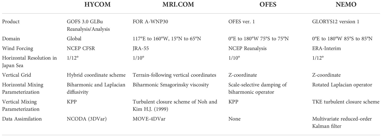
Table 1 Fundamental configurations of four models assessed in this study, including the information on assessed product, the wind forcing dataset, the horizontal and vertical grid schemes, the parameterization schemes, the data assimilation method, and the model domain.

The HYCOM is a primitive equation OGCM that develops from the Miami Isopycnic-Coordinate Ocean Model, which is widely used for ocean climate studies (Halliwell et al., 1998; Halliwell et al., 2000; Bleck, 2002). HYCOM employs hybrid vertical coordinates, reverting smoothly from isopycnals in stratified open seas to z-level coordinates in mixed layers and further to terrain-following coordinate in weak stratification areas. A tri-pole latitudinal grid is employed as horizontal coordinate in which all 1D submodels are embedded. The used vertical mixing parameterization is K-Profile Parameterization (KPP) (Large et al., 1994). Lateral advection and diffusion of salinity, temperature, and momentum were presented by a combination of biharmonic and Laplacian diffusivity. The bulk formula of Kara et al. (2000) is used for heat flux parameterizations. The sea ice thermodynamics are simulated by energy loan ice model. Atmospheric forcing data are the 1-hourly National Centers for Environmental Prediction (NCEP) Climate Forecast System Reanalysis (CFSR) data, which has a spatial resolution of ~38 km. In Global Ocean Forecast System (GOFS) 3.0, the temperature and salinity profiles, altimeter SSH, and satellite SST were assimilated by the Navy Coupled Ocean Data Assimilation (NCODA) using 3D variational (3DVar) assimilation scheme. Outputs of the GOFS3.0 forecast system include daily 3D temperature, salinity, currents, and 2D SSH. To ensure a consistent time period with other models, we selected GOFS 3.0 Glbu Reana lysis data from 1993 to 2013 and extend the time span to 2015 by supplying the GOFS 3.0 GLBu Analysis data. The GOFS 3.0 Glbu data has 40 vertical layers with a horizontal resolution of 1/12°. The vertical resolution reduces from 2 m near the sea surface at 1,000 m to the bottom at 5,500 m.

The Meteorological Research Institute Community Ocean Model (MRI.COM) is a multilevel primitive equation model with hydrostatic and Boussinesq assumptions. It was used for large-scale simulations of oceanic phenomena as an ocean component of coupled climate models (Ishikawa, 2005; Tsujino et al., 2006). The 4D variational (4DVar) Ocean Re-Analysis for the Western North Pacific over 30 years (FORA-WNP30) is used in this study, which is the output of the western North Pacific version of the MRI Community Ocean Model (MRI.COM-WNP) (Usui et al., 2017). The configurations of MRI.COM-WNP are fundamentally consistent with MRI.COM (Tsujino et al., 2006) except for denser bottom layers and incorporation of sea-ice model. The horizontal mixing of tracers and momentum were parameterized by a biharmonic operator and biharmonic Smagorinsky viscosity, respectively. The vertical viscosity and diffusivity were provided by the turbulent closure scheme from Noh and Kim (1999) after eliminating the dependency of vertical mixing coefficients and bottom friction on the background state. Heat fluxes were obtained from bulk formula (Kondo, 1975). The model domain covers the Northwest Pacific zonally from 117°E to 160°W and meridionally from 15°N to 65°N. MRI.COM uses terrain-following vertical coordinates. There are 54 vertical layers with the interval increasing from the surface at 1 m to the bottom at 600 m. Horizontally, MRI.COM-WNP applied variable grid scheme for a cost-effective simulation of the Northwest Pacific circulation at high resolution, setting zonal resolution of 1/10° from 117°E to 160°E and 1/6° from 160°E to 160°W and meridional resolution of 1/10° from 15°N to 50°N and 1/6° from 50°N to 65°N. The in situ temperature and salinity profiles above 1,500 m, gridded SST, altimeter SSH, and sea ice concentration data were assimilated into MRI.COM-WNP by using 4DVar analysis scheme version of the MOVE system (MOVE-4DVar) with the first Gauss from the analysis fields of MOVE-3DVar. Previous evaluation studies shows that FORA-WNP30 incorporated with MOVE-4DVar has higher accuracy than the 3DVar product (Usui et al., 2017). Atmospheric forcing was taken from daily JRA-55 atmospheric reanalysis product with a regular horizotal grid of ~0.56° resolution (Kobayashi et al., 2015). Boundary conditions were created by a North Pacific model with a horizontal resolution of 1/2° using a one-way nesting method (Hirose et al., 2016).

The OFES is based on the MOM version 3 for a long-term, eddy-resolving hindcast of the global ocean circulation with the available supercomputing resources. OFES utilizes the vertical z-level coordinate and solves 3D primitive equations in the horizontal spherical coordinates under hydrostatic and Boussinesq approximations. The domain of OFES model is a quasi-global region from 75°S to 75°N excluding the polar regions. The horizontal resolution is 0.1°. The number of vertical layers is 54 from 2.5 to 6,065 m with the intervals varying from the surface at 5 m to the bottom at 330 m. The horizontal mixing of momentum and tracers was parameterized by scale-selective damping of biharmonic operator to suppress computational noise. The vertical mixing parameterization used KPP (Large et al., 1994). The bulk formula of Rosati and Miyakoda (1988) is used to calculate surface heat flux. The OFES-based hindcast experiments were initialized by the 50-year climatological spin-up integration (Masumoto et al., 2004). Atmospheric forcing is obtained from daily NCEP/NCAR reanalysis products (Kalnay et al., 1996). The hindcast products of OFES1 was assessed in this study.

The NEMO is a state-of-the-art modeling framework in ocean and climate sciences (Madec, 2008). The ocean engine of NEMO (NEMO-OCE) is a primitive equation model intended to be used for modeling studies on the ocean and its interactions with the earth climate system in various spatiotemporal scales (Madec et al., 2017). As a state-of-the-art representative of NEMO-based products, the GLORYS12 version 1 reanalysis product generated by the PSY4V3 forecast system based on NEMO 3.1 (Lellouche et al., 2018; Jean-Michel et al., 2021) is used in this study. NEMO 3.1 for GLORYS12 adopts rotated Laplacian operator for the horizontal parameterization of both tracers and momentum advection, and the TKE turbulent closure scheme is used for the vertical mixing parameterization (Lellouche et al., 2018). A quasi-isotropic grid was utilized in the horizontal direction, and a z-coordinate is applied in the vertical. The horizontal resolution of GLORYS12 is 1/12°. There are 50 vertical layers from the surface at 0 m to the bottom at 5,700 m. The model is driven by the European Center for Medium-Range Weather Forecasts ERA-Interim atmospheric reanalysis (Dee et al., 2011). A multivariate reduced-order Kalman filter is applied to assimilate temperature and salinity profiles provided by the Coriolis Ocean Dataset for Reanalysis (CORA), altimeter SSH and AVHRR satellite SST in a 7-day assimilation cycle (Lellouche et al., 2018). In the present study, we use an overlapping period of 1993–2015 for all the four models.

2.2. Observations

2.2.1. Temperature and salinity profiles

To evaluate the physical conditions simulated by the selected eddy-resolving ocean circulation models, we took the temperature and salinity profiles collected by the Conductivity Temperature Depth (CTD) from 1993 to 2014 via 19 research cruises conducted through the CREAMS (Circulation Research of the East Asian Marginal Seas) and EAST-I (East Asian Seas Timeseries I) and 59 cruises conducted by the Japan Meteorological Agency. The CTD stations cover most areas of the northern (Figure 1, square dots) and southeastern Japan Sea (Figure 1, triangle dots). All CTD data were carefully calibrated based on raw data except for those collected by cruises from 1999 June to 2000 February, for which only preliminarily processed data are available. They were processed by using standard procedures, such as those of the Sea-Bird Electronics (SBE). Most CTD data collected after 2002 were processed by pre-cruise and post-cruise calibrations following the typical SBE data processing sequences (Morison et al., 1994). Ancillary temperature and salinity along five geostationary observation lines from 1968 to 2021 were taken from the Korea Oceanographic Data Center (KODC). The KODC data were sampled bimonthly or more frequently, whereas Japan Meteorological Agency (JMA) and CREAMS/EAST-I data had more irregular sampling intervals (Kang et al., 2008). For the present study, we selected hydrographic data from the monitoring stations C1 (134.0°E, 41.5°N) and C2 (132.3°E, 42.2°N) in the Japan Basin, J1 (136.7°E, 39.5°N) and J2 (134.4°E, 38.7°N) in the Yamato Basin, as well as K1 (130.9°E, 37.9°N) and K2 (130.6°E, 36.5°N) in the Ulleung Basin. These locations are illustrated by green dots in Figure 1. The selected stations cover conditions in the northern, the southeastern, and the southwestern Japan Sea and differ primarily in the influence of ocean current, thermal conditions, and atmospheric conditions. All profiles were preprocessed into standard depths with a vertical resolution of 2 m from 0 m to 5,000 m. For each in situ measurement data, the collocated model data were selected by searching and averaging in a 3-day time window and a spatial radius of 1/6°. A 30-day moving average has been applied on both the time series of collocated observation and model data to eliminate small-scale noise and focus on the mean state and obtain monthly time series.

2.2.2. Ocean current

For the assessment of surface circulation, we used the gridded Drifter ocean current product as the ground truth. After the launch of Global Drifter Program in 1979, a total number of 907 buoys were deployed by various institutions in the Japan Sea, covering at least 80% of the total area (Wang et al., 2020). Each Drifter buoy carries a floating anchor at 15 m to record its real-time location and transmit raw data through the Global Telecommunication System. The buoy trajectories reflect the near surface current velocities because the impact of wind-driven current and Stokes flow has been minimized, and the actual Drifter velocity data are composed of geostrophic velocity, Ekman velocity, and other non-geostrophic velocity.

For the evaluation of simulated ocean current, we used the velocity measurements from Acoustic Doppler Current Profiler (ADCP) at two long-term monitoring stations: the EC1 located near the offshore branch of the EKWC and the East Sea Real-time Ocean Buoy (ESROB) located near the longshore branch of the EKWC (Figure 1, red pentagons). The EC1 is a deep mooring buoy deployed to the north between Ulleung and Dok Islands in 1996 during a cooperative experiment conducted by the Korea Ocean Research and Development Institute, the Woods Hole Oceanographic Institution, and the Seoul National University (SNU). It works autonomous and is equipped with various instruments at 400, 1,400, and 2,000 m (Chang et al., 2002), which records hourly velocity data from 1993 to present. The ESROB is a long-term, continuous, and real-time ocean monitoring buoy maintained by the SNU Ocean Observation Laboratory to observe multiple oceanographic phenomena and processes in the Japan Sea (Kim et al., 2005). It is deployed 10 km off the coast at a depth of ~100 m from 1999 to present. ESROB is equipped with 300-kHz ADCP and several SBE37 CTDs to measure 3D subsurface currents and hydrographic properties at 26 vertical layers for every 1 to 10 min.

For the present study, we used ADCP hourly current velocity data from 2000 through 2014. The 15-year period is well overlapped by each ocean current models. We selected the EC1 data at 400 m and ESROB data at 5, 20, 40, 60, and 100 m, respectively, where the largest amount of velocity data was collected. To compare with the ADCP data, the model data were taken from 3D fields at approximately the same location and depth as the EC1 and ESROB stations.

2.2.3. Surface wind velocity

To estimate the deviations of four atmospheric wind forcing datasets—the Climate Forecast System Reanalysis (CFSR) for HYCOM, the Japanese 55-year Reanalysis (JRA-55) for MRI.COM, the NCEP/NCAR Reanalysis 1 (NCEP R1) for OFES, and the ERA-Interim for NEMO, we compared these reanalysis data with the QuikSCAT sea surface wind product. For the comparison purpose, both reanalysis and satellite products were interpolated into daily time series with a consistent spatial resolution of 0.25°.

2.2.4. Taylor diagram

The Taylor diagram, which presents three statistical evaluation parameters in one semicircle or quarter chart, including the Pearson correlation coefficient, the standard deviation, and the root mean square deviations (RMSDs), is employed for this assessment. The Pearson correlation coefficient quantifies the similarity between the observed and simulated time series. It is represented by straight lines related to the azimuthal angle. Values from 0 to 1 indicate from no correlation to 100% agreement. The normalized standard deviation of each model time series relative to the observations was calculated to obtain a unified representation of deviations in one Taylor diagram. This value is proportional to the radial distance from the origin of the Taylor diagram, which indicates the similarity between the amplitude of simulated and observed time series. The centered RMSD in the Taylor diagram is proportional to the distance from the corresponding arc with the x-axis. See the study by Taylor (2001) for a detailed description on Taylor diagram. The closer distance represents the smaller RMSD of simulated time series relative to the observation result.

2.2.5. Extended cost function

As the offsets between the time series of simulated and observed data are not included in the Taylor diagram, we defined an extended cost function as an additional measure for the quality assessment of simulated time series. According to Eilola et al. (2011), the original cost function (C) was computed for each model (i) by

where the M_i indicates the monthly simulated time series and O indicates the monthly observed time series. STD is the standard deviation of observational data. The cost function values were calculated at each depth to evaluate the similarity between observations and simulations. Values between 0 and 1 indicate good agreement, values between 1 and 2 indicate reasonable quality, and values larger than 2 reveal poor quality. Therefore, a good accordance is defined by the fact that the deviation between observed and simulated time series is smaller than twice the STD values of observation time series. On the basis of the normalized STD, the Pearson correlation coefficient and the RMSD given by the Taylor diagram, an extended cost function value is defined as follows

where STD_i and RMSD_i represent the standard deviation and RMSD of simulated time series, respectively.

2.3. Evaluation strategies

To assess the capacity of four eddy-resolving ocean circulation models to reproduce long-term mean state of physical and hydrographic environment in Japan Sea, a 22-year time period from 1993 through 2014 was selected. First, the quality of simulated temperature and salinity data is evaluated by comparing the corresponding model reanalysis products with in situ measurements provided by JMA cruises in the southeast, CREAMS/EAST-I cruises in the north, and KODC monitoring stations in the southwest. The evaluation process includes the validation of vertical profiles and the statistical comparison of time series at different depths of the selected monitoring stations.

Next, the simulated sea surface current velocities throughout the Japan Sea and the volume transport into three major straits were evaluated. Note the assessment of middle and deep circulation patterns is not in the scope of this study as model simulations in deep layers tend to contain large errors in Japan Sea with inadequate data assimilation and sparce vertical model layers in deep ocean. In addition, we also analyzed the vertical structure of simulated ocean currents across the major straits. Locations of three transactions used for the calculation of volume transport are marked as blue lines in Figure 1. The Tartar Strait, located at the northern end of the Japan Sea with more than 10 km width, is excluded from this study due to the negligible volume transport.

Finally, the current velocities simulated by four eddy-resolving ocean models were compared against ADCP measurements at two monitoring stations, and the atmospheric wind forcing data driving the ocean models were analyzed and compared with satellite wind product from QuikSCAT.

3. Results

3.1. Temperature and salinity at monitoring stations

3.1.1. Mean vertical profiles

Figure 2 shows the 22-year mean vertical temperature and salinity profiles along with their standard deviations at six typical monitoring stations. Both the mean values and standard deviations were calculated from the monthly time series between January 1993 and December 2014. The mean temperatures at these stations vary from approximately 1°C to 18°C with the maximum standard deviations of ~5°C near sea surface. The near surface temperature from 0 to 100 m is well reproduced by each model at almost each station with the maximum deviations no larger than 1°C. However, the exception occurs at the station C2 where 0–40 m is a positive error and 40–80 m is a significant negative error. The temperature is slightly overestimated at station C1 by all models except HYCOM and is slightly underestimated at station K2 by HYCOM. In addition, OFES has worse performance at almost each station except the K2 station with both significant positive and negative biases.

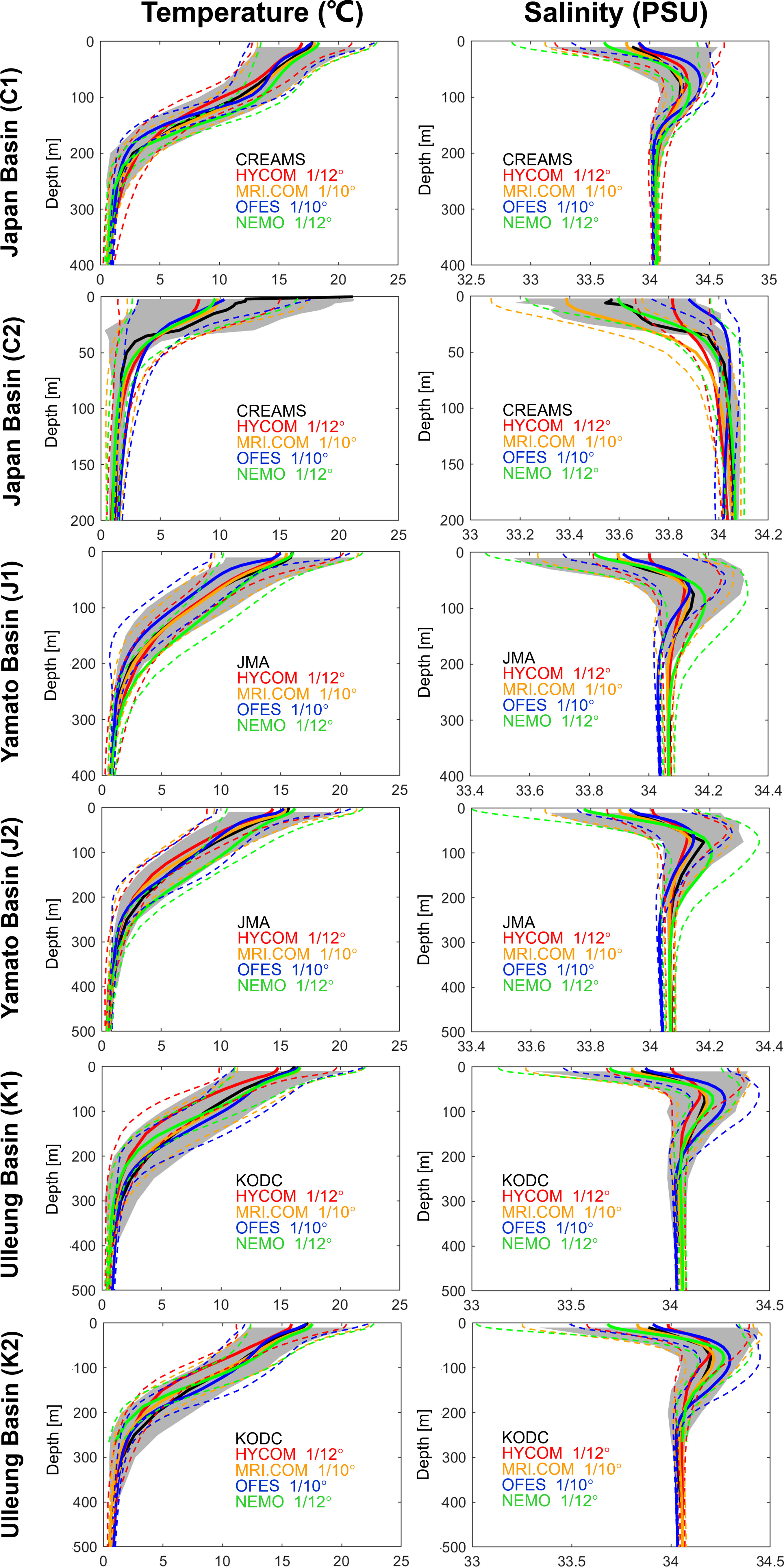
Figure 2 Mean vertical profiles of temperature (left) and salinity (right) observed by six representative stations (black) and simulated by four eddy-resolving ocean models HYCOM (red) and OFES (blue) with 1/12° resolution, MRI.COM (orange) and NEMO (green) with 1/12° resolution with 1/2° resolution for the time period from 1993 through 2014. Results for the monitoring stations C1 and C2 in the Japan Basin, J1 and J2 in the Yamato Basin, and K1 and K2 in the Ulleung Basin are displayed from bottom to top. Mean values are illustrated by solid lines. Standard deviations are indicated by the gray-shaded area for the observation data and by the colored dashed lines for the models.

At all stations, the temperature monotonously decreases with depth, but the thermocline stretches at different vertical locations depending on each station. For most stations, the thermocline simulated by NEMO lies 10–30 m lower than that observations from six stations. Below the thermocline, each model almost perfectly fits to the observations at all stations with the deviations no larger than 1°C. The standard deviations of temperature at very large depths are smaller than 1°C for both simulations and observations.

The 22-year mean salinity values range from approximately 33.6 to 34.3 g kg⁻¹ at the sea surface, whereas, at the bottom, the salinity values are highly concentrated near ~34.05 g kg⁻¹. At most stations, the standard deviations of salinity are much smaller than 0.3 g kg⁻¹. Exceptions occur at the sea surface of C1 station, at 0–30 m depth of C2 station and the sea surface at K2 station, where the maximum standard deviations all exceed 0.5 g kg⁻¹. The mean salinity simulated by four models rarely exceeds the range of observed standard deviations. However, almost all models fail to reproduce the upper salinity structure at C2 station, which significantly bends at 40 m depth instead of smoothly stretches from sea surface to 70 m depth. Among them, the negative biases of HYCOM and MRI.COM at 30–80 m and the positive biases of OFES at 30 through 70 m slightly exceed the range of observed standard deviation. Moreover, NEMO presents the location of salinity thermocline at relatively low depths, especially at the southeastern stations J1 and J2. At very large depths, an overestimation can be noticed from NEMO at C2 station, whereas OFES undersetimates the deep salinity of all stations by the magnitude of 0.05 g kg⁻¹.

In summary, the mean temperature and salinity simulated by MRI.COM are partly beyond the range covered by the standard deviation of observation, whereas the means simulated by HYCOM and NEMO exceed the observed standard deviations more often than MRI.COM at various stations and depths. Moreover, HYCOM has an overall better performance than NEMO in simulating both temperature and salinity profiles. By contrast, the OFES data are in relatively poor quality especially in terms of salinity at very large depths. It is possibly due to the absence of data assimilation in OFES model to correct the simulated profiles at those monitoring stations.

3.1.2. Statistical assessment

To further assess the capacity of four models to simulate the temporal variations of temperature and salinity at six stations, the Taylor diagram and the extended cost function are applied here. Figure 3 shows the Taylor diagram of upper ocean temperature and salinity relative to the observation data as the black reference point located on the x-axis (normalized standard deviation = 1, Pearson correlation coefficient = 100%). The Taylor diagram of temperature shows high consistency between simulated and observed profiles at each station. The Pearson correlation coefficients of SST are generally higher than 0.7. Among them, the MRI.COM values at surface to subsurface reach as high as 0.95, and the normalized standard deviations for temperature are closest to 1 at J1, K1, and K2 stations.

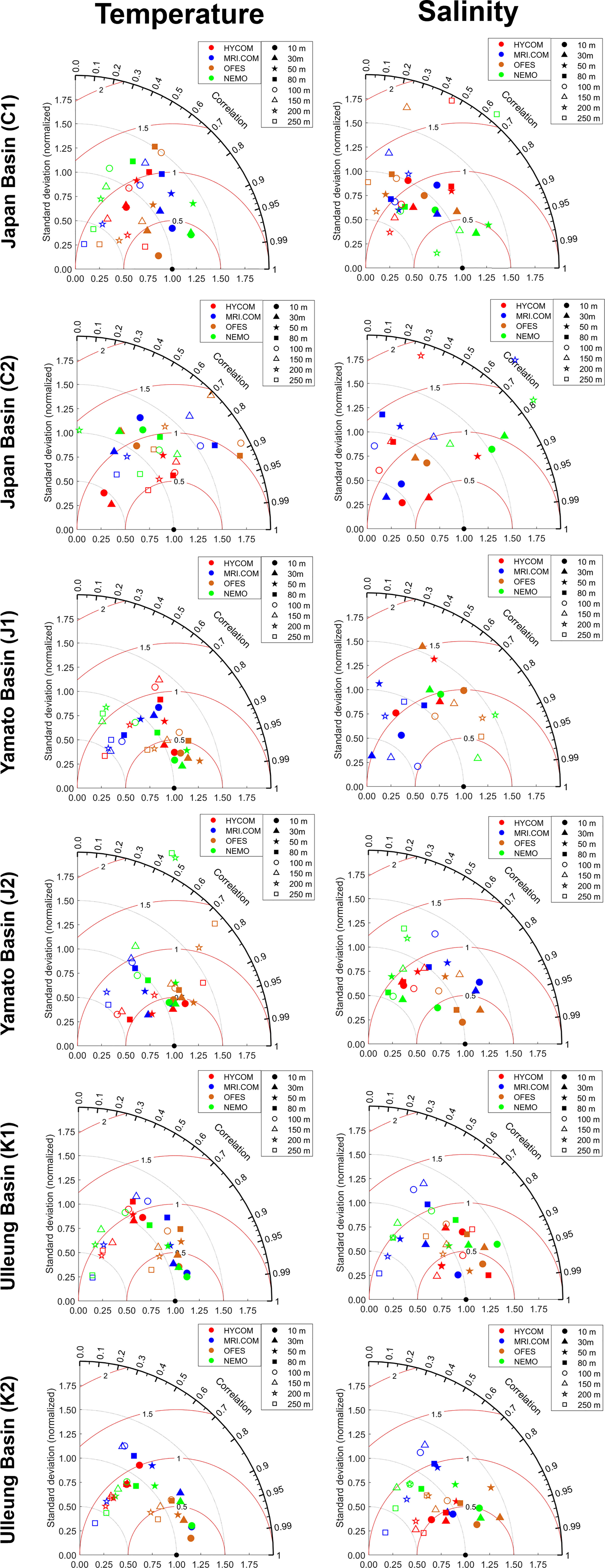
Figure 3 Taylor diagrams plotted from monthly time series of temperature (left) and salinity (right) from 1993 to 2014 at standard depths at the monitoring station C1 and C2 in the Japan Basin, J1 and J2 in the Yamato Basin, and K1 and K2 in the Ulleung Basin. Correlation, normalized standard deviation, and centered RMS difference of the simulated time series from the ocean models HYCOM (red) and NEMO (green), MRI.COM (orange), and OFES (blue) compared with the observational data are shown. Different markers refer to different standard depths. See text for more details.

The cost function in Figure 4 further verifies that eddy-resolving ocean circulation models can well reproduce the temperature profiles at each station. At almost every depth, the cost function values of temperature lie between 0 and 1, indicating good data quality. Below 100 m, different models begin to show diversified capacities to simulate the temperature at different depths. MRI.COM presents the overall smallest cost function values, which are mainly distributed between 0 and 0.5 with a few large deviations below 50 m at the C2 station. This proves the very good quality of SST data simulated by MRI.COM. The temperature cost function values are generally smaller than 1 and are maximized for OFES at 200 m depth of C2 station, for HYCOM at the surface of C2 station, and for NEMO at 200 m depth of the J2 station. At the above locations, the cost function values are larger than 1.5, which represents reasonable data quality. It is noted that all the four models have the lowest cost function values at C2 station, which corresponds to the obvious deviation of simulated profiles in Figure 2.

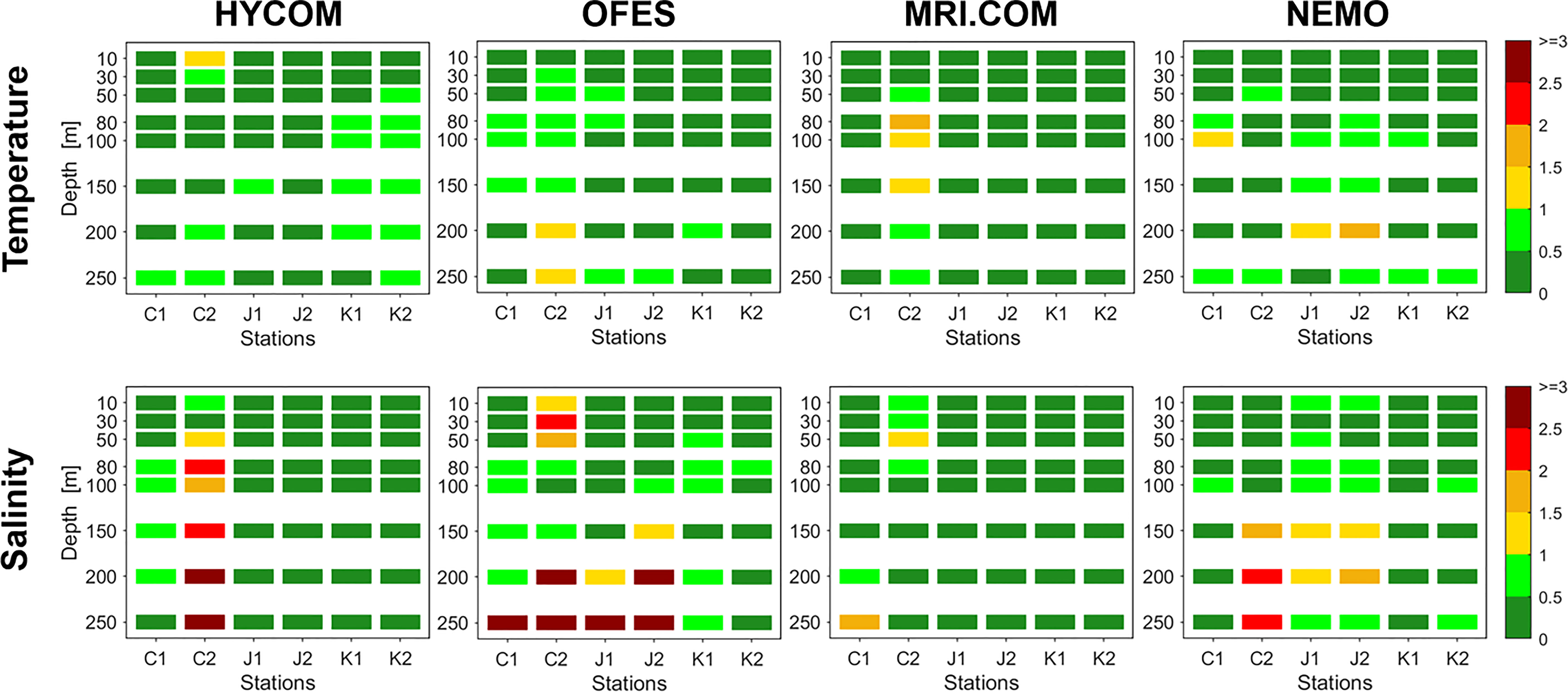
Figure 4 Values of Cost function derived from monthly time series of temperature (top) and salinity (bottom) from 1993 to 2014 at the six representative monitoring stations. Results from the ocean models HYCOM, OFES, MRI.COM, and NEMO (from left to right) compared with the observation data are shown at the same depths as illustrated in the Taylor diagrams in Figure 3. See text for more details.

The Taylor diagrams and cost function values reveal stronger differences of salinity among four eddy-resolving ocean models. MRI.COM has the overall best performance at almost each station with the highest correlations, the smallest spread of the normalized standard deviation around the observation value of 1, as well as the smallest RMSD values appearing in almost all depths. Most cost function values are significantly smaller than 0.5, indicating a very good accordance of salinity reanalyzed by MRI.COM with the observation data.

The statistics of salinity reproduced by HYCOM and NEMO are comparable to each other with the overall data quality of HYCOM slightly higher than that of NEMO. Their correlation coefficients are mainly between 0.5 and 0.95. Most deviations from the normalized standard deviation of 1 are no more than 0.5, and the RMS errors lie predominantly between 0.5 and 1.3. The cost functions are predominantly no larger than 1.5 but still reveal the shortcomings of two models in reproducing salinity at certain depths and stations.

Comparatively, OFES has the overall worst performance of salinity simulations, which is reflected by the generally lower correlation coefficients (most below 0.8), the higher deviations from the normalized standard deviation of 1 (up to about 0.7 in deep layers), and the highest RMS errors (up to 1.4) in the Taylor diagrams. Similarly, the cost function values are higher in OFES than in other models, indicating a poor agreement between OFES simulations and observations. It is interesting to note that MRI.COM and NEMO are complementary to each other in the salinity data quality at most stations, especially the C2, J1, and J2 stations. Moreover, it can be concluded from the hydrographic simulation results of four models that the spread of cost function values for temperature is smaller than that of salinity.

The mean cost function values for temperature and salinity also support the above results. As shown in Table 2, MRI.COM presents the lowest values, indicating the best data quality. The cost function values of HYCOM and NEMO are mid-table, whereas OFES presents the highest cost function values that indicate the lowest data quality.

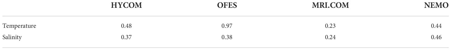
Table 2 Average cost function values for temperature and salinity based on Equation 2 for the ocean models HYCOM, OFES, MRI.COM, and NEMO.

3.1.3. Long-term variability

We further analyzed temperature and salinity at near-surface depths of the ESROB station, including the 5, 20, 40, 60, and 100 m depths for both models and observations. Figure 5 shows the time series of monthly mean temperature from 2000 to 2014 and that for salinity is shown in Figure 6. During this period, the observed temperature varies from 5°C to 25°C with the minimum occurring in winter and maximum appearing in summer, and the range of observed salinity extends from 33 g kg⁻¹ in summer to 34.5 g kg⁻¹ in winter. In upper layers, the seasonal variations of both temperature and salinity have much stronger magnitudes than that of interannual variations. As the depth increases, the interannual variations become more pronounced in both ESROB observations and model simulations, which even overtake the magnitude of seasonal variations at 100 m depth. This conforms to the fact that subsurface water is less affected by the surface wind and heat flux forcing with strong seasonal variations (Byju et al., 2018). For both temperature and salinity, it is interesting to note that OFES agrees very well with the ESROB data both in magnitude and variability, whereas MRI.COM has an unexpectedly worse performance. Sudden changes in temperature and salinity, for instance, at the beginning of 1994 or 1998 are reproduced very realistically. At deeper layers, the differences between observation and simulation data become significantly larger.

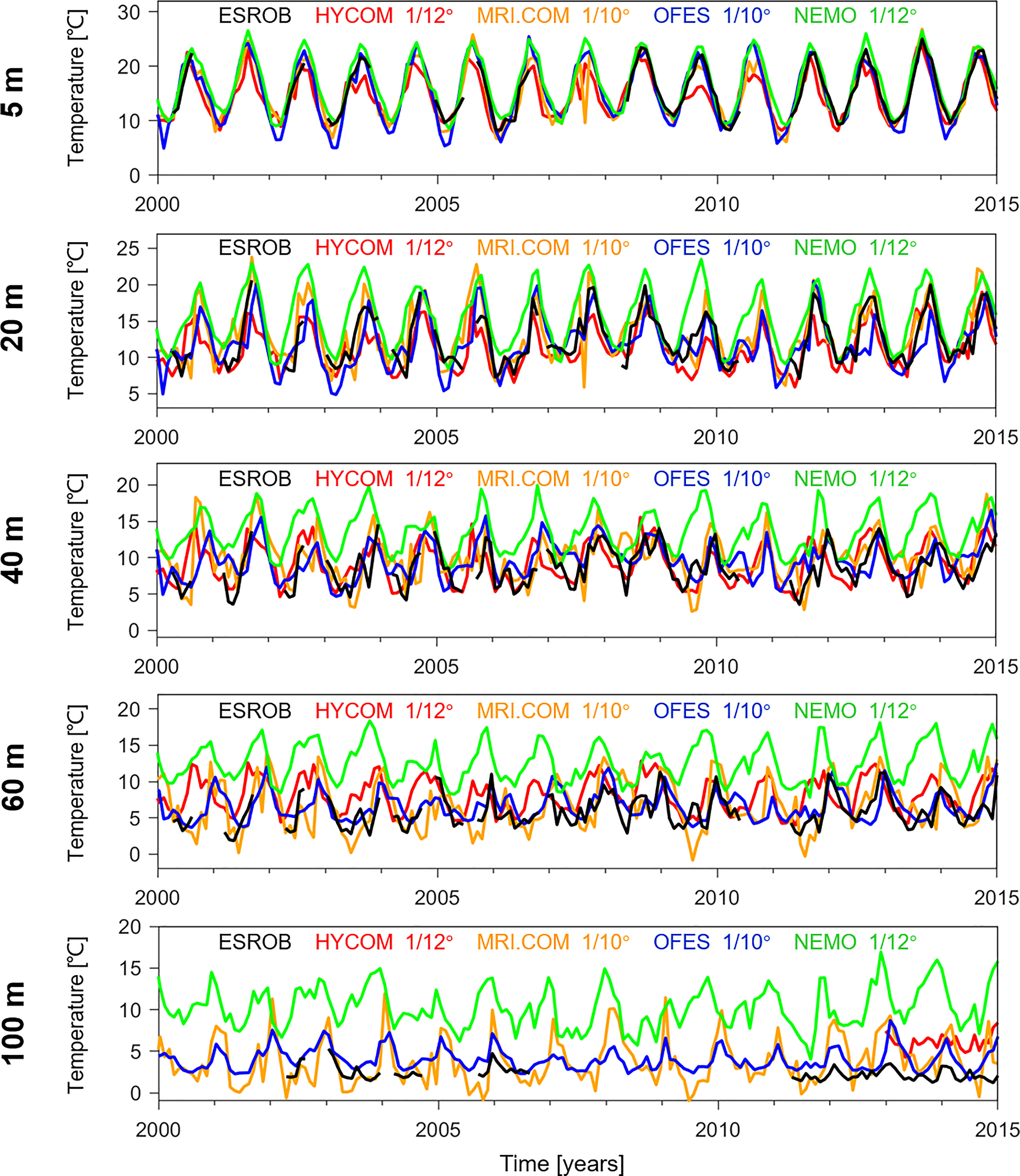
Figure 5 Monthly mean temperature from ESROB observation data (black) and the ocean models HYCOM (red), MRI.COM (orange), NEMO (green), and OFES (blue) at 5, 20, 40, 60, and 100 m depths for the time period from 2000 to 2014.

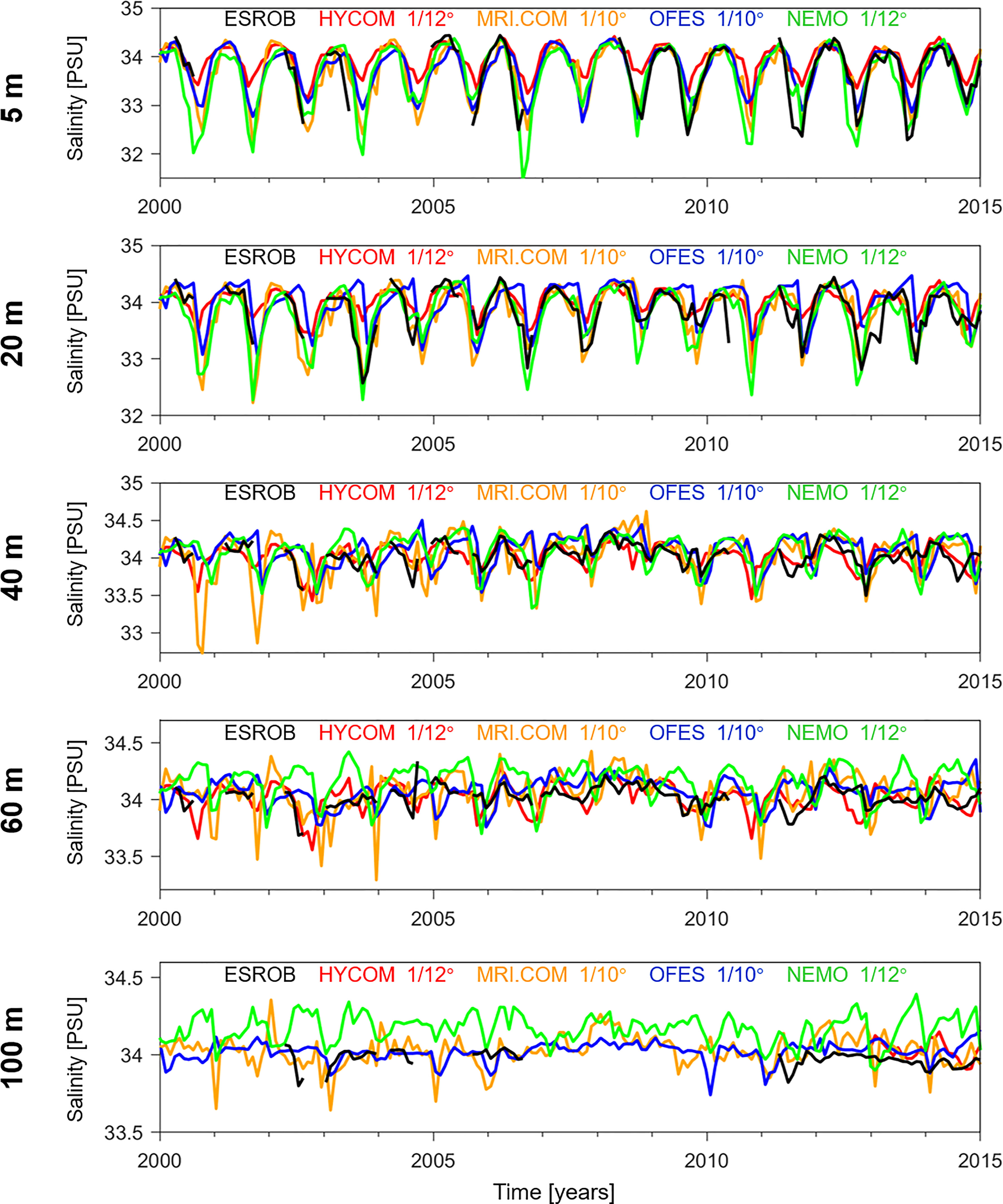
Figure 6 The same as Figure 5 but for the monthly mean salinity.

The HYCOM and MRI.COM models partly reproduce the observed magnitudes very well but do not show the reasonable variations that are visible in the ESROB and OFES data. They overestimate or underestimate temperature at each depth from time to time by up to 5°C. NEMO generally overestimates the temperature by a maximum from 1°C at sea surface to 9°C at 100 m. Salinity at each depth is well reproduced by HYCOM, OFES, and MRI.COM with maximum deviations from the observations of no more than 0.3 g kg⁻¹. The best accordance of models and observations occurs at sea surface where OFES and MRI.COM simulate the observed seasonal variations precisely. Again, NEMO still presents the largest deviations compared with ESROB data, especially in deep layers where the maximum exceeds 0.5 g kg⁻¹ from time to time.

3.2. Mean circulation

3.2.1. Horizontal surface circulation patterns

A comparison with Drifter ocean current at 15 m is conducted to evaluate the surface circulation patterns simulated by the four eddy-resolving models. The ocean current structure observed by Drifter buoys at 15 m is shown in Figure 7. Statistics show that most sea surface areas of the Japan Sea are covered by current velocities varying from 0 to 0.3 m s⁻¹. Maxima velocity of up to 1 m s⁻¹ appears around the Tsugaru Strait, up to 0.4 m s⁻¹ in the Tsushima Strait, and up to 0.4 m s⁻¹ in Peter the Great Bay. The majority of large flows that were previously observed in the Japan Sea has been well depicted by Drifter data, including the Liman Cold Current (LCC) along the Russia coast, the Nearshore Branch (NB), and Offshore Branch (OB) near the Japan coast, the EKWC and North Korea Cold Current (NKCC) along the Korea coast, as well as the SubPolar Front Current (SPFC) in the middle and wind-driven current near Vladivostok.

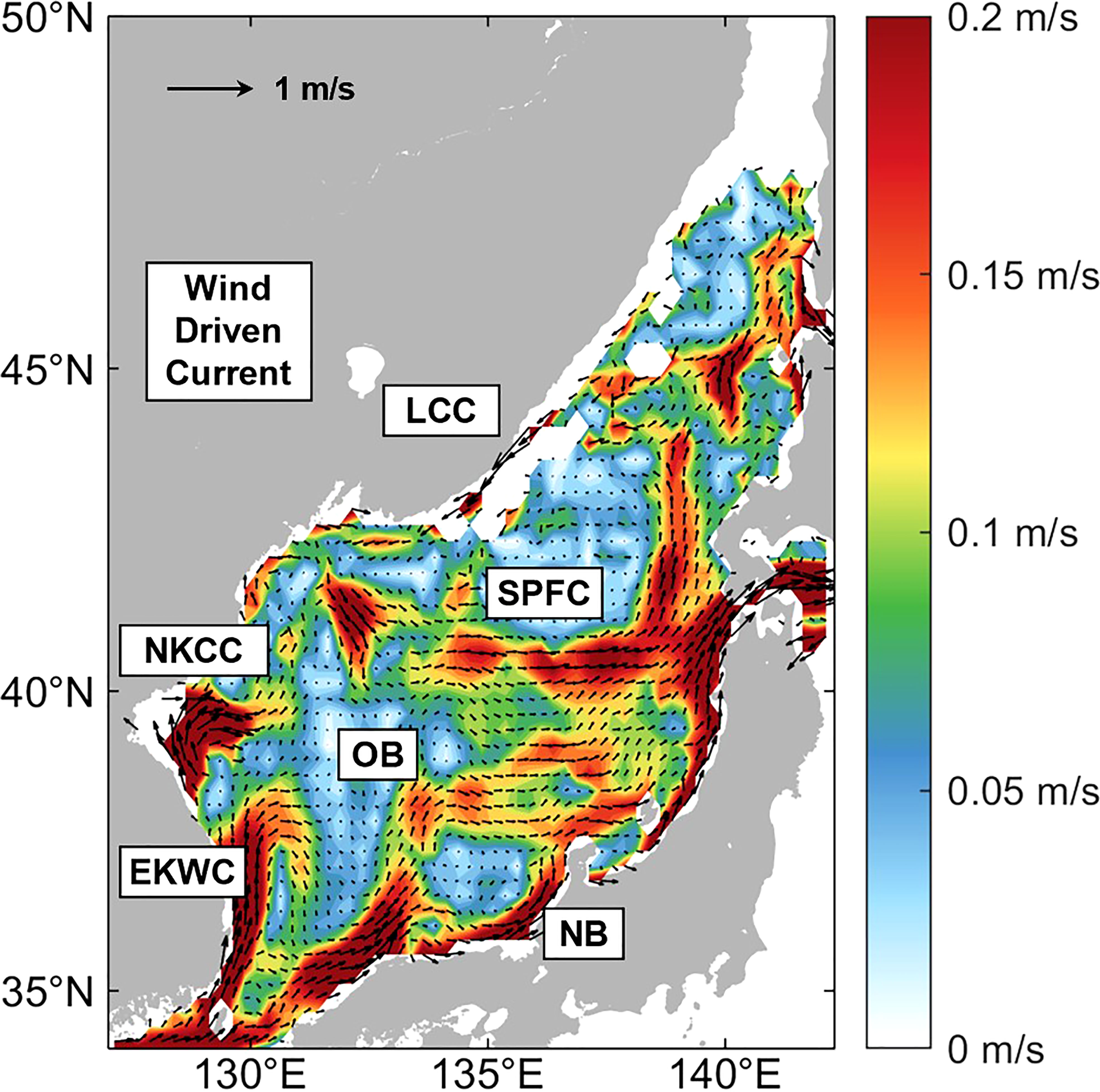
Figure 7 The climatological ocean circulation patterns at 15 m depth as represented by the Drifter interpolation dataset with the major flows labeled by white boxes. EKWC, East Korea Warm Current; NKCC, North Korea Cold Current; NB, Nearshore Branch; OB, Offshore Branch; SPFC, SubPolar Front Current; LCC, Liman Cold Current.

The left column of Figure 8 shows the difference in surface current velocities between model simulations and Drifter data. The overall strength of the surface circulation throughout the Japan Sea has been underestimated by all models as indicated by the large blue areas. Generally, most models have underestimated the strength of EKWC in the East Korea Bay and the SPFC at the south boundary of Japan Basin. Compared with other models, the difference between the 15-m current velocities simulated by MRI.COM and that observed by Drifter buoys shows relatively smaller deviations of about −0.30 m s⁻¹ in maximum and −0.05 m s⁻¹ on average. HYCOM and NEMO differ stronger with Drifter surface currents throughout the whole Japan Sea with the maximum deviation of −0.76 and −0.69 m s⁻¹, respectively. Both models overestimate the strength of NB along the whole Japan coast, but HYCOM underestimates the strength of the EKWC near the Korea coast, whereas NEMO tend to overestimate it. OFES still has the largest difference with Drifter. OFES simulates mainly smaller current speeds than other models. The average deviation is −0.07 m s⁻¹, and the maximum negative difference is approximately −0.94 m s⁻¹. The middle and right columns of Figure 8 show the differences in warm season (June through August) and cold season (December through February). The statistics are generally consistent between cold and warm seasons with similar distribution of bias values. The largest discrepancy appears south of Vladivostok where strong winter monsoon flows across the mountain gap, brings strong wind-driven current, and causes larger differences between simulated and observed current velocities. This is possibly related to the sparce resolution of wind forcing data because the monsoon and wind-driven current occupy a small area near the northwest coast of Japan Sea.

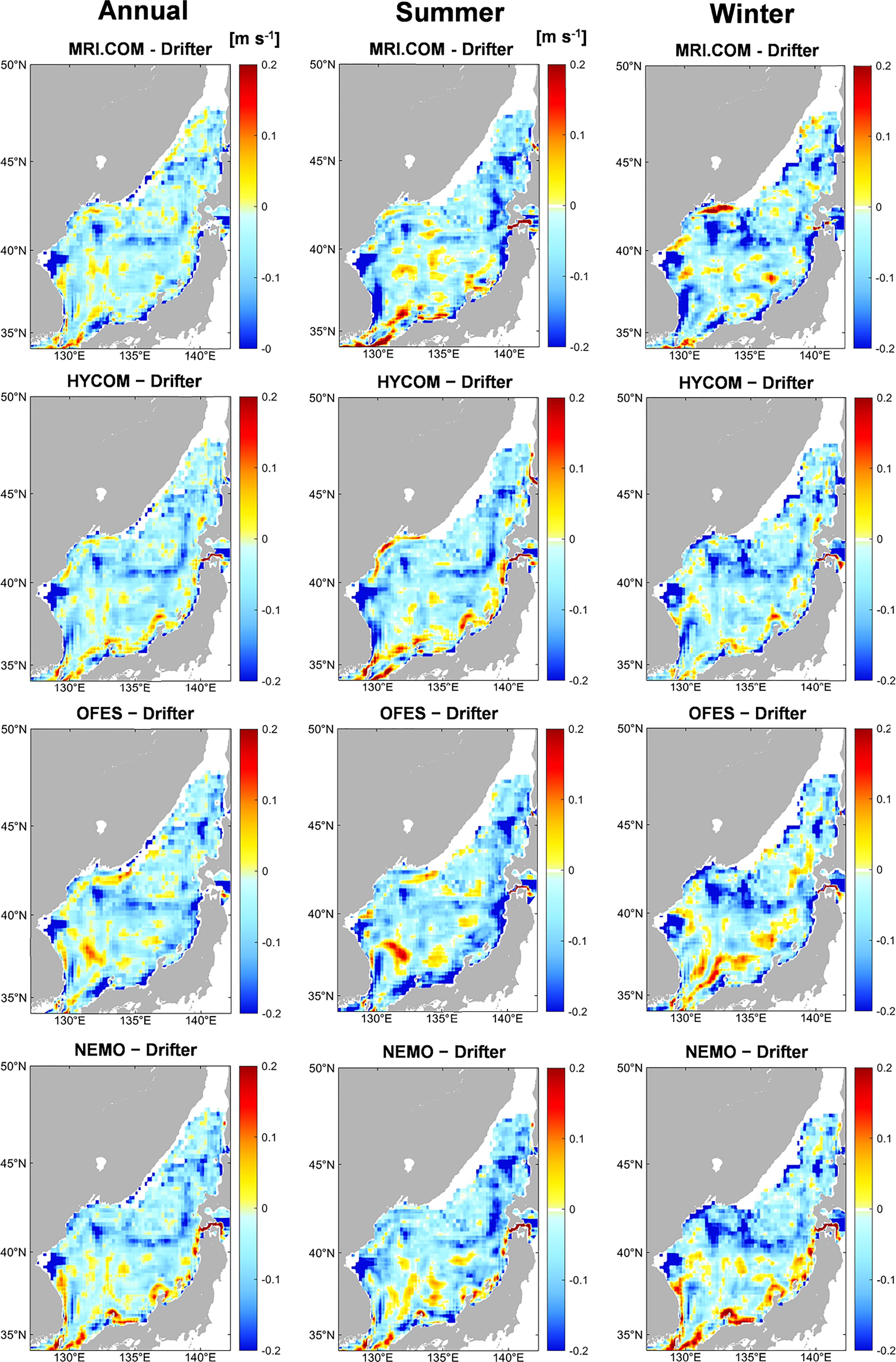
Figure 8 Twenty-two–year mean surface velocity at 15 m for the years 1993 through 2014, including the annual mean (left), the summer mean (middle), and the winter mean (right). The panels from top to bottom show the differences of the individual models MRI.COM, HYCOM, OFES, and NEMO from the Drifter reference data, respectively.

3.2.2. Current velocity through major straits

Figure 9 shows the average current velocities through the three major straits as simulated by four eddy-resolving ocean circulation models. Positive values indicate eastward currents for the Tsugaru and Soya Strait and northeastward currents for the Tsushima Strait, respectively.

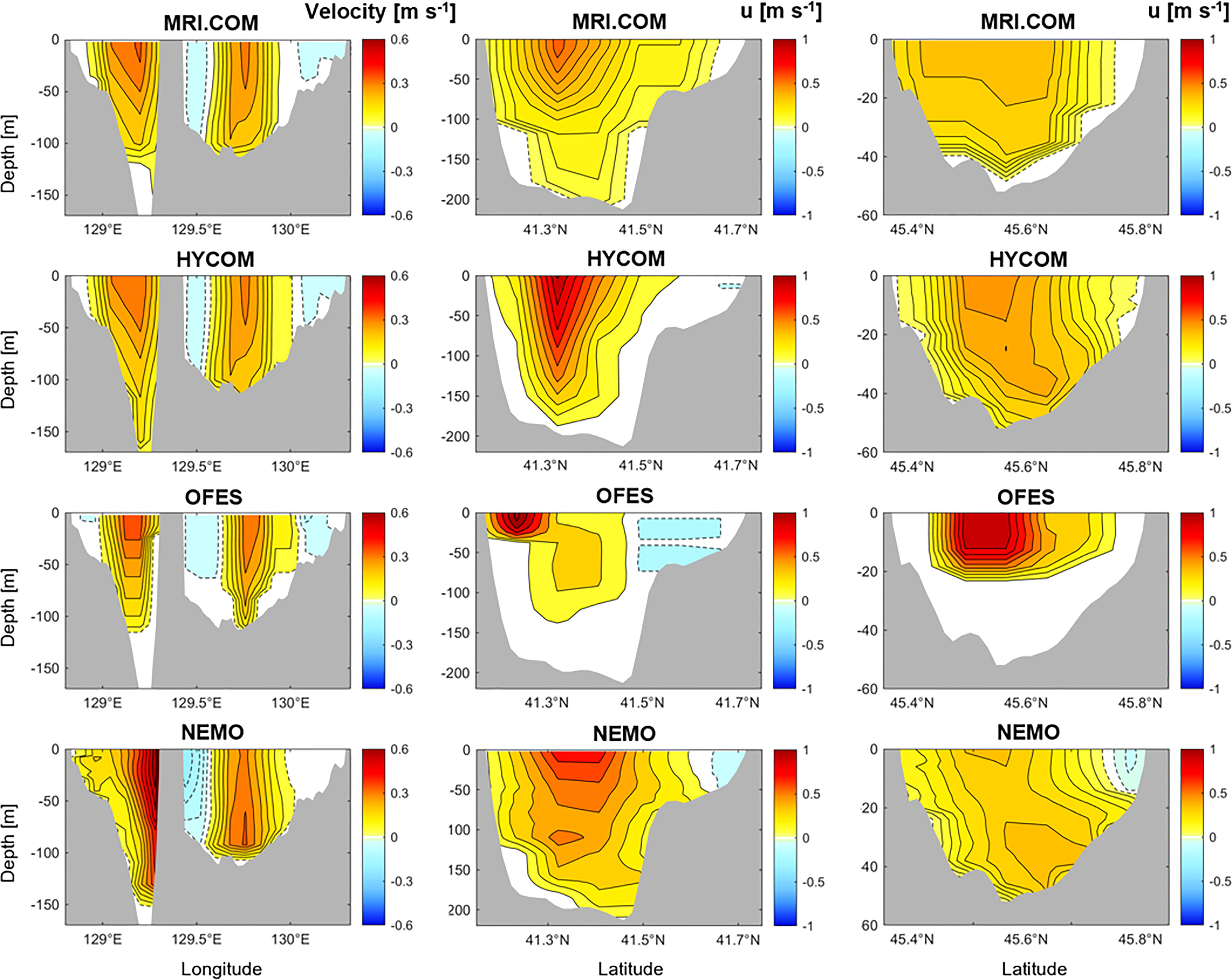
Figure 9 Mean current velocity profiles across the Tsushima Strait (left), Tsugaru Strait (middle), and Soya Strait (right) for the time period from 1993 to 2014 for the models MRI.COM, HYCOM, OFES, and NEMO. Positive values denote northeastward velocity for Tsugaru Strait and eastward velocity for Tsugaru Strait and Soya Strait. Isolines are solid for positive values and dashed for negative values. Note that the shown profiles cover different ranges of depth. The contour interval is 0.1 m/s for each graph.

The 22-year mean zonal velocity through the Tsushima Strait as simulated by all the four models shows a bifurcation structure in the downstream region and a weak countercurrent near the Tsushima Island. Generally, the current is northeast directed (positive) in the middle part of both channels maximizing approximately between 0 and 50 m depth at about 0.5 m s⁻¹ for MRI.COM and OFES and 0.4 m s⁻¹ for HYCOM. In the west channel, the current velocity simulated by HYCOM, MRI.COM, and OFES is generally consistent, with the maximum speed of 0.4 m s⁻¹ appearing in the middle part of the sea surface. However, NEMO describes a very distinct flow pattern with a maximum of 0.9 m s⁻¹ and a strong flow core located near 25 m depth very close to the coastline. Near the Tsushima Island in the east channel, the current is southward directed (negative) and the negative velocities range from 0 m at the surface to 90 m at the bottom, which is also overestimated by NEMO. The middle part of the east channel is characterized by a northeastward current near the sea surface with a maximum of 0.4 m s⁻¹. Near the Japan coast is the southwestward-directed (negative) current extending to the bottom. However, for NEMO, the velocities are negligible whereas HYCOM, MRI.COM, and OFES simulate a maximum velocity about 0.1 m s⁻¹. Overall, the currents simulated by NEMO are stronger than HYCOM, MRI.COM, and OFES. The vertical profile simulated by four models is comparable to that observed by ADCP (Ostrovskii et al., 2009) except for the common overestimations of velocity in the east channel.

The zonal current through the Tsugaru Strait is predominantly eastward (positive) over the whole transect with a maximum of 0.5–1.3 m s⁻¹ depending on each model. MRI.COM simulates the weakest current throughout the transect with a maximum of 0.5 m s⁻¹. HYCOM and NEMO simulate comparatively stronger magnitudes than MRI.COM with the maximums appearing at the same location. OFES simulated the strongest current, but large velocities are mainly distributed near the southern coast with a narrow range both horizontally and vertically. This is not necessarily due to the 1/10° horizontal resolution of OFES because the MRI.COM model with the same horizontal resolution also captures the narrowest transect across the Tsugaru Strait, which shows similar distributions of velocity compared with HYCOM and NEMO. Nor it is likely due to the z-coordinates adopted by OFES in shallow water because reasonable simulation results are found in the Tsushima Strait, where the lateral boundaries are steep for z-coordinates. It is likely because OFES assimilates no observational data, or, possibly, it is related to the fact that the bathymetries near each strait are individually adapted to the numerical solvers of each numerical model. Similar to the Tsugaru Strait, the zonal currents through the Soya Strait reveal a unidirectional throughflow structure with a strong flow core in the middle of the sea surface. The velocity direction is predominantly eastward with the maximum of 0.5 m s⁻¹ for MRI.COM and NEMO, 0.6 m s⁻¹ for HYCOM, and 1.0 m s⁻¹ for OFES. In principle, the patterns simulated by MRI.COM and NEMO are similar with HYCOM having slightly stronger magnitudes. OFES simulates the throughflow with a significant shift to the west and with stronger current velocities but smaller meridional and vertical ranges than the other models.

3.2.3. Volume transport through main straits

Figure 10 shows the simulated 22-year average vertical profiles of volume transport per unit depth that are integrated horizontally along the three straits each. For the Tsushima Strait, the vertical profiles of MRI.COM, HYCOM, and NEMO are highly similar with maximum inflows of about 30,000 m² s⁻¹ at sea surface, whereas OFES has the weakest magnitudes (the maximum is around 20,000 m² s⁻¹) but similar distributions. In the upper layers, all models simulate inflows into the Japan Sea with OFES having the narrowest horizontal and vertical ranges.

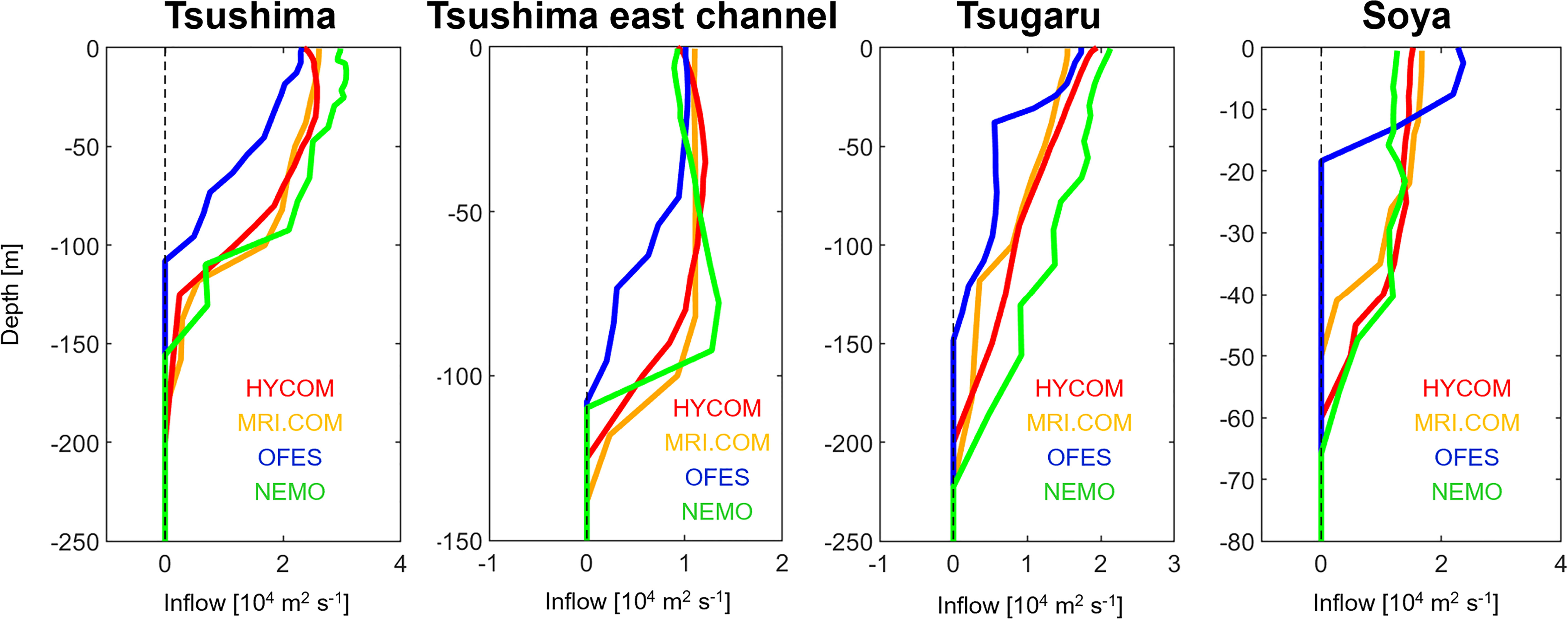
Figure 10 Vertical profiles of horizontally integrated velocities per unit depth along the Tsushima Strait, Tsugaru Strait, Soya Strait, as well as along the east channel of the Tsushima Strait only (between Tsushima Island and Japan) as simulated by the ocean models HYCOM (red), MRI.COM (orange), NEMO (green), and OFES (blue) for the time period from 1993 to 2014.

When only the east channel of the Tsushima Strait is considered, the vertical profiles greatly differ from the profiles for the whole strait. Because of the exclusion of northeastward inflow in the east channel, the Tsushima Strait east transect is characterized by a weaker inflow into the Japan Sea over the whole depth and the vertical range decreases from 170 m for the whole transect to no more than 150 m for the east channel. The almost unchanged and even increased volume transport per unit depth between the surface and 90 m depth simulated by HYCOM, MRI.COM, and NEMO is partly caused by the weakened countercurrent at the eastern coast near the Tsushima Island, which is strongest pronounced in NEMO near the sea surface. Therefore, NEMO maximizes in about 12,000 m² s⁻¹ at 80 m depth. At a shallower depth of 40 m, HYCOM and MRI.COM reveal maximum inflows of about 11,000 and 10,000 m² s⁻¹, respectively, whereas OFES simulates maximum inflow of only 9,500 m² s⁻¹ at the sea surface.

At the Tsugaru Strait, the vertical structure of volume transport per unit depth is, in principle, comparable to that at the Tsushima Strait except for the weaker magnitude. Because of the deeper topography, the flow range extends further down to the 200 m depth, but the maximum outflow still occurs near the sea surface for all models. The outflow magnitudes reach from almost 20,000 m² s⁻¹ for NEMO to about 15,000 m² s⁻¹ for HYCOM and MRI.COM and only 13,000 m² s⁻¹ for OFES. The flow range extends down to 110 m for OFES, 210 m for NEMO, and 190 m for HYCOM and MRI.COM.

The mean vertical profiles of volume transport per unit depth at the Soya Strait have a similar shape with that of Tsushima and Tsugaru Strait. Maximum outflow from the Japan Sea to the Northwest Pacific takes place near the sea surface and extends to the depth of about 50 m for MRI.COM, 60 m for HYCOM, and 65 m for NEMO, but only 20 m for OFES. These are consistent with the current velocities illustrated by Figure 9. The maximum outflow ranges from almost 22,000 m² s⁻¹ for OFES to about 17,000 m² s⁻¹ for HYCOM and MRI.COM and 16,000 m² s⁻¹ for NEMO.

In addition, the 22-year mean depth-integrated volume transport per unit length in three main straits is shown in Figure 11. For the Tsushima Strait, the volume transport simulated by each model is predominantly northeastward directed (positive) between Korea and the western coast of the Tsushima Island. The magnitudes for MRI.COM and HYCOM are generally the same, whereas OFES simulates a smaller transport and NEMO simulates a larger transport. Between the eastern coast of the Tsushima Island and Japan, a countercurrent structure is visible with southwestward transport along the eastern coast of the Tsushima Island, whereas the rest transport is dominantly northeastward directed. Here, the transports differ very slightly among the four models with the maximum close to 35 m² s⁻¹. For the Tsugaru Strait and Soya Strait, the whole transects are dominated by eastward (positive) outflow with the volume transport differing greatly in both magnitude and meridional distributions. The maximum outflow ranges from almost 40 m² s⁻¹ for OFES to about 130 m² s⁻¹ for HYCOM in the Tsugaru Strait, whereas, in the Soya Strait, there is a narrower range from 15 m² s⁻¹ for OFES to about 27 m² s⁻¹ for MRI.COM. Note that, compared with other models, MRI.COM simulates a significantly larger proportion of outflow through the Soya Strait, and a rather smaller proportion is allocated to the Tsugaru Strait.

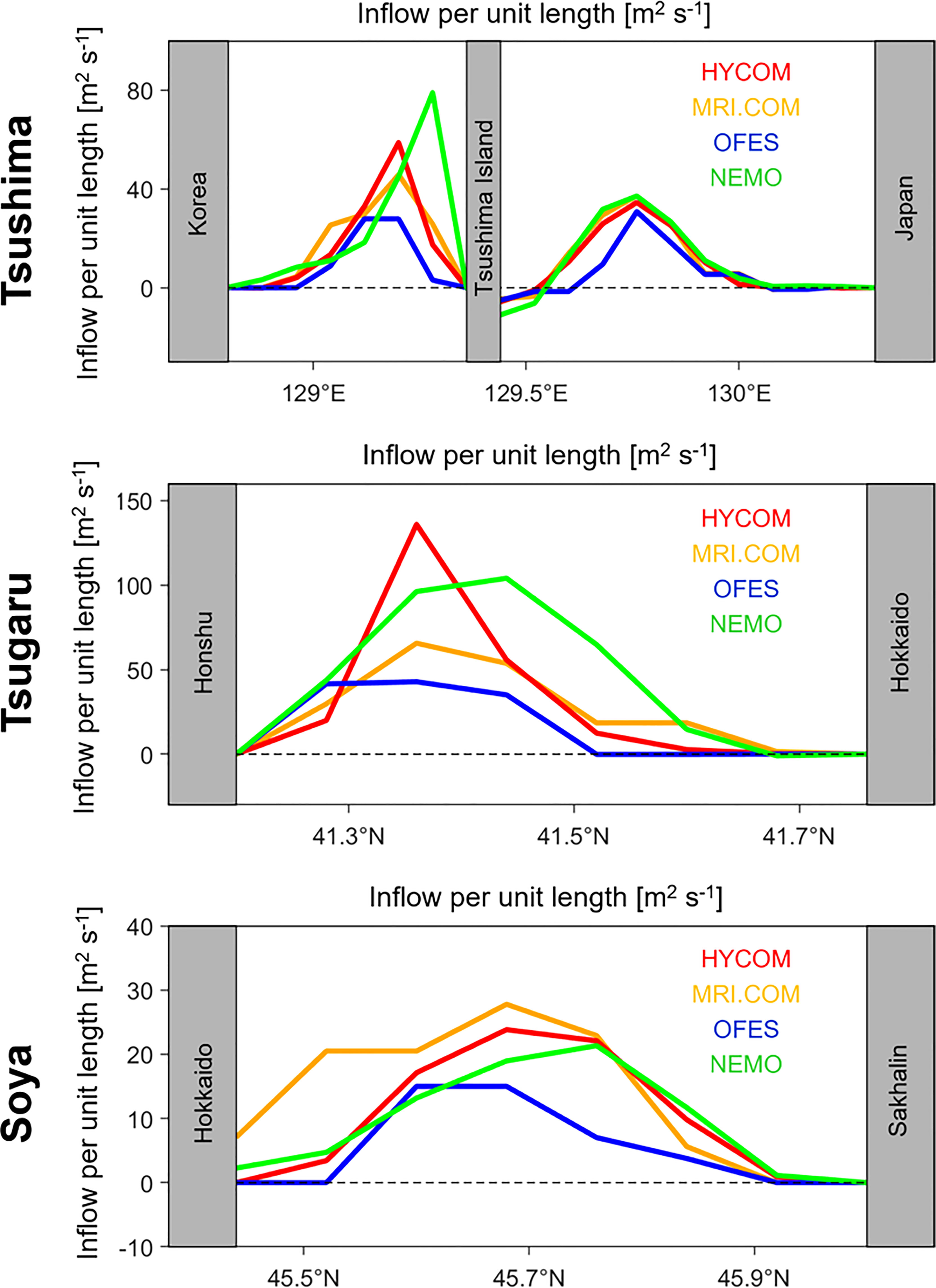
Figure 11 Depth-integrated velocities per unit length orthogonal across three major straits as simulated by the ocean models HYCOM (red), MRI.COM (orange), OFES (blue), and NEMO (green) for the time period from 1993 to 2014.

We further analyzed the water balance through Japan Sea straits as simulated by four models between 1997 and 2008. The observed volume transport data are taken from ADCP measurements (Fukudome et al., 2010) in the Tsushima Strait and sea level difference across the Tsugaru Strait (Han et al., 2016). The observed volume transport is unavailable in the Soya Strait due to the lack of a tide gauge on the north side and the insufficient ADCP measurements. Figure 12 shows the differences between the transport entering the Japan Sea and the transport flowing out through the Tsugaru Strait and the Soya Strait from the observation data and four model simulations. All models reach a fine balance between the inflow transport into the Tsushima Strait and outflow transport into the Tsugaru and Soya Strait with the in-out differences smaller than 0.2 × 10⁶ m³ s⁻¹. Among them, OFES shows an underestimation of total transport by ~0.8 × 10⁶ m³ s⁻¹, NEMO slightly overestimates by ~0.2 × 10⁶ m³ s⁻¹, whereas both HYCOM and MRI.COM transport are comparable with the observations. The proportion of outflow transport through the Tsugaru Strait has been overestimated by each model, which is close to 55% from observation data but has exceeded 70% from the simulations of four models. The above suggests that simulations of numerical models satisfy the physical conservation of volume transport, but the allocation of outflow transport between the Tsugaru and Soya Strait cannot reach an agreement with the observations.

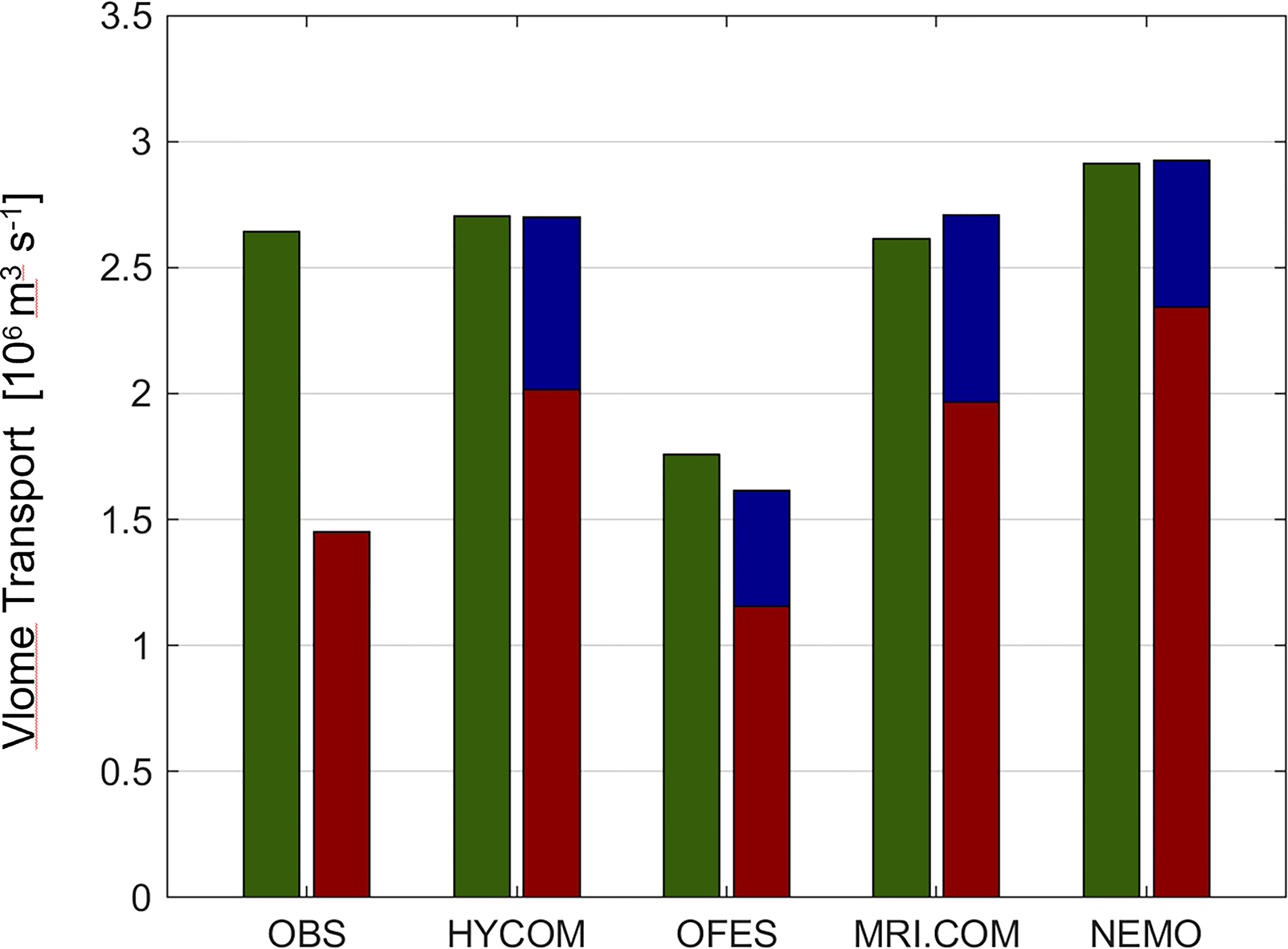
Figure 12 Differences between the volume transport entering the Japan Sea through the Tsushima Strait (green) and the outgoing transport through the Tsugaru (red) and Soya/La Perouse (blue) Straits for observed data, reanalyses from the four models, and consolidated estimations.

3.3. Evaluation of current velocities

The current velocities simulated by each model were validated against the mooring ADCP measurements at ESROB and EC1 stations, which locate at the axis of the longshore EKWC branch and the offshore EKWC branch, respectively.

3.3.1. ESROB

The statistics of ADCP data are shown on the left-hand side of Figure 13 labeled by black markers, which are calculated from monthly time series at 20 m depth below the sea surface. The 10-year mean observed zonal current velocity is close to 1.5 cm s⁻¹ with a standard deviation of about 6 cm s⁻¹. Each model simulates a similar magnitude of zonal current, but the standard deviations vary from 3 cm s⁻¹ for HYCOM to 12 cm s⁻¹ for NEMO. The relative frequency of the observed and simulated zonal currents shows a very good agreement with similar mean values and consistent spread. Note that a few outlier values of ADCP between −0.3 and −0.4 cm s⁻¹ are not included in this histogram.

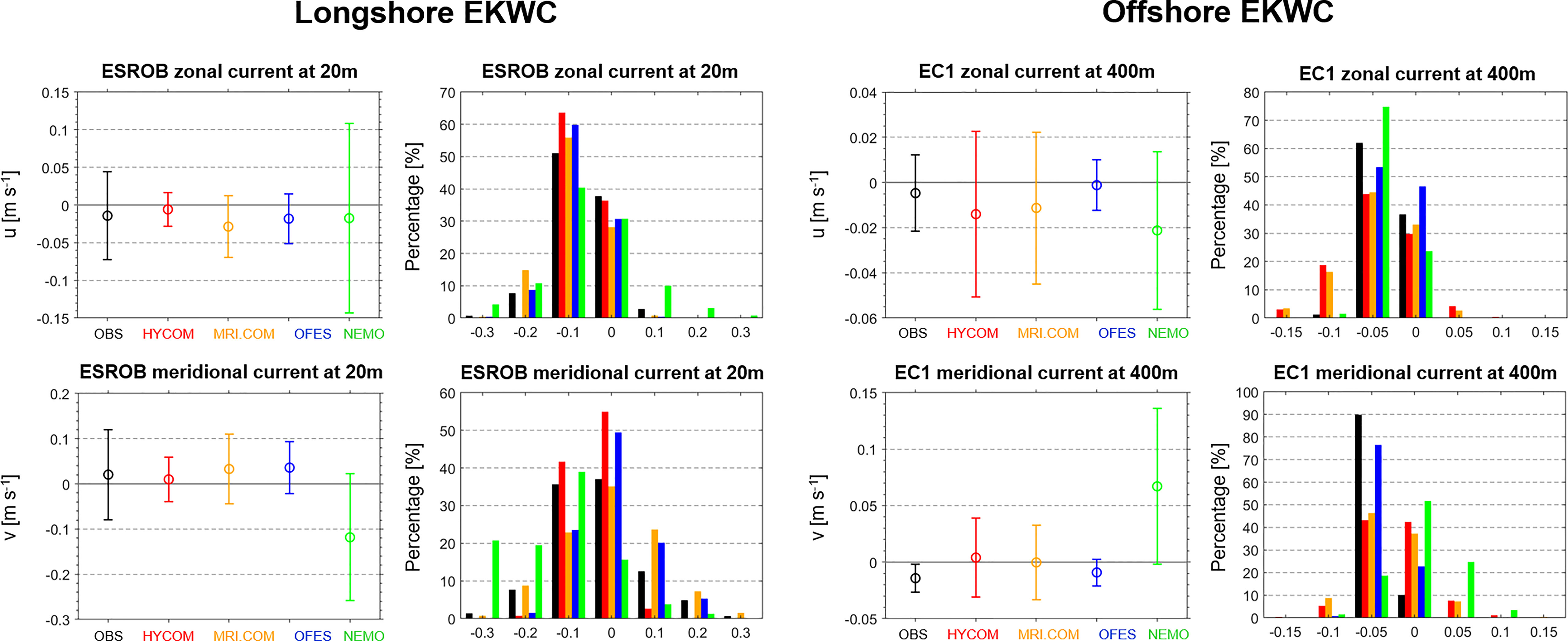
Figure 13 Mean current velocities with their standard deviations as well as relative frequency of these velocities from geostationary observations (black) from and model simulations (colors) at 20 m depth of the ESROB station located near the longshore branch of EKWC (left) and at 400 m depth of the EC1 located near the offshore branch of EKWC (right). Results for zonal components are shown in the top panels and for meridional components in the bottom panels. See text for further information.

The mean meridional current velocities observed and simulated at 20 m depth are less in accordance with each other. The ADCP measurements are distributed around the mean value of 2 cm s⁻¹ with a standard deviation of about 10 cm s⁻¹. MRI.COM and OFES lie very close to these values. HYCOM shows a similar variation with the observations but varies around the mean value of 1 cm s⁻¹. NEMO has a distinct mean value of about −11 cm s⁻¹, and the standard deviation is much higher, which is almost twice as large as that of ADCP data. The relative frequency values reflect good agreement of each model with ADCP measurements, except for the NEMO model that presents significantly larger relative frequency values.

3.3.2. EC1

The statistics of ADCP observations at the EC1 station near the offshore branch of EKWC are shown on the right-hand side of Figure 13, which are similarly based on monthly averaged data, but at the depth of 400 m. NEMO still has a poor performance in simulating both the zonal and meridional current velocities with very different mean values and standard deviations. For the rest three models, the 15-year mean meridional current velocities and the standard deviations are very close to zero for both the ADCP observations and model simulations. The small range of deviation is also reflected by the large relative frequency from −5 to 0 cm s⁻¹. Larger discrepancies between ADCP measurements and model simulations occur for the zonal current velocities. From the ADCP data, it varies around the mean value of −0.5 cm s⁻¹ with a standard deviation of about 1.5 cm s⁻¹. OFES has most similar mean values and variation range with ADCP. In contrast, HYCOM and MRI.COM models simulate larger mean values (~−1.5 cm s⁻¹) and standard deviations larger than 6 cm s⁻¹.

3.4. Evaluation of atmospheric forcing data

Finally, the wind velocities of ERA-Interim, CFSR, NCEP R1, and JRA-55, which drive the ocean circulation models, are evaluated by a comparison with QuikSCAT satellite data. The mean statistics over the whole Japan Sea, which are considered for this assessment, have been summarized in Table 3. They reveal partly substantial differences between QuikSCAT data and reanalysis forcing data. The average zonal wind from both observations and reanalysis is eastward directed with generally the same magnitude. The mean meridional wind is southward directed and reanalysis data reproduce similar magnitudes with observations. However, the wind speed averaged over the whole Japan Sea is significantly underestimated by each reanalysis dataset with the largest differences and RMSDs that occur for CFSR (HYCOM) and ERA-Interim (NEMO). In addition, the standard deviations, both for the component speed and total speed, are larger in observations than in reanalysis. Note that the smaller differences for JRA-55 (MRI.COM) and NECP R1 (OFES) correspond to the smaller deviations of MRI.COM and OFES current velocities with Drifter data.

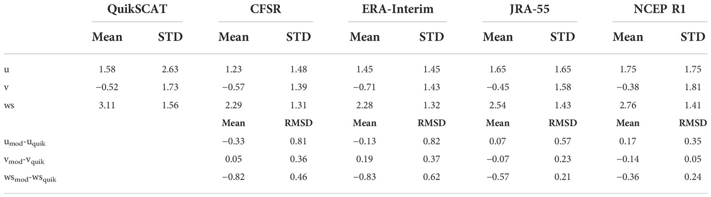
Table 3 Mean zonal wind speed (u), meridional wind speed (v), and total wind speed (ws) together with their standard deviations for QuikSCAT, CFSR, ERA-Interim, JRA-55, and NCEP R1 dataset, as well as the mean and root mean square deviation (RMSD) between the reanalysis datasets (mod) and the satellite observations (quik) for the zonal, meridional, and total wind speed.

The annual cycle and standard deviations of wind speed averaged throughout the whole Japan Sea are illustrated in Figure 14. Generally, all the four reanalysis datasets agree well with the QuikSCAT observations, but reanalysis datasets systematically underestimate the magnitude of mean wind speed, especially in autumn and winter months when the northwest monsoon prevails over the Japan Sea. NCEP R1 and JRA-55 are closer to the satellite observations but still underestimate the mean wind speed in autumn and winter and slightly overestimate it in May and July.

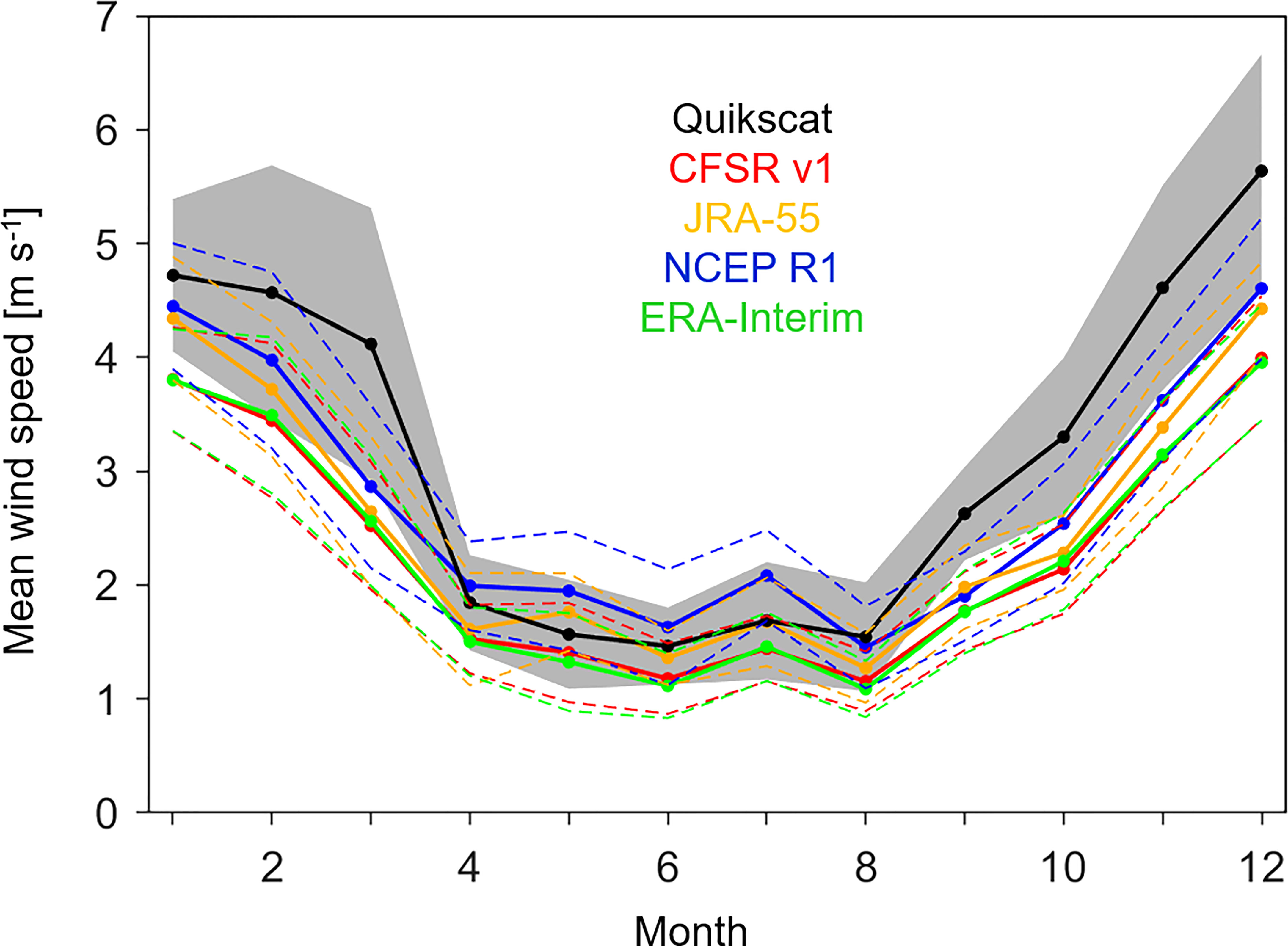
Figure 14 Annual cycle of monthly mean wind speed over the Japan Sea for the observations (black), CFSR v1 (red), JRA-55 (yellow), NECP R1 (blue), and ERA-Interim (green). The solid lines indicate the monthly mean and the shading indicates ±1 standard deviation.

4. Discussions

In this assessment, the overall best simulation performance of temperature and salinity profiles is found for MRI.COM-WNP, a North Pacific regional ocean circulation model using the MOVE-4DVar data assimilation scheme to ingest a large amount of in situ measurements in Japan Sea. The temperature and salinity profiles utilized for this assessment belong to the World Ocean Database 13 (WOD13), which is a subset of the assimilation database for MRI.COM-WNP. Compared with the other three models with vertically adaptive coordinates, OFES and NEMO have the disadvantage of applying z-coordinates in the vertical direction, which may generate spurious mixing across the isopycnals (diapycnical mixing) in the interior of the ocean (Gräwe et al., 2015) especially in Japan Sea where steep sea floors are widely distributed. This unreal numerical mixing might result in the anomalous thermocline structures and mixed layer depths (Figure 2). However, the thermocline reproduced by OFES is less biased than NEMO, which is possibly because the OFES model adopts a scale-selective damping of biharmonic operator to suppress the spurious computational noise. This opens the possibility to explore the effects of applying the biharmonic operator in NEMO to improve the parameterizations for surface waves and Langmuir circulation. Although numerical mixing is also present in HYCOM and MRI.COM, this mixing might mimic the effects of physical mixing and, therefore, corresponds better to the in situ observations than the deep water mixing parameterizations used in z-coordinate models.

Because of the assimilation of a very large volume of in situ temperature and salinity measurements in the Japan Sea, we assume that the baroclinic current velocity fields simulated by MRI.COM are closest to observations. However, the barotropic currents, which are driven by the wind stress curl minus the bottom friction curl, are not influenced by data assimilation and, consequently, not constrained by temperature and salinity measurements.

In the following, several hypotheses related to the diversities in both hydrographic and dynamical conditions among four ocean circulation models are proposed:

1. Because all models tend to reproduce temperature much better than salinity, it is induced that the calibration of heat balance is easier than that of water balance in the Japan Sea. However, there are detailed differences among different eddy-resolving models. Largest deviations in temperature are found from OFES and NEMO data possibly because the z-coordinates are not well simulating the vertical mixing processes. In contrast, smaller biases are found for MRI.COM and HYCOM, which applies terrain-following coordinates in the shallow water.

2. Mean surface velocities in the southern part of the Japan Sea, where most large surface currents are distributed, are significantly stronger in NEMO than in the other models. A possible explanation is the zooming of vertical layers toward the sea surface in NEMO. The minimum layer thickness can reach 1 m, and there are more than 20 layers above 100 m, which enables a better representation of the wind shear effect on the upper layers. Whether the stronger barotropic velocities simulated by NEMO are more realistic than that simulated by other models cannot be determined as mentioned above. Because OFES also has dense layers near the sea surface but simulates a weaker barotropic circulation in the south part than MRI.COM, either the bottom fraction or the horizontal viscosity in OFES is significantly larger than in MRI.COM. Moreover, all the four models have underestimated the ocean current at 15 m compared with Drifter observations, especially near the Peter the Great Bay where wind-driven current is dominant. The possible reason behind might be the weaker wind speeds of the atmospheric forcing in each model compared with the reality.

3. Compared with the other five stations, both the temperature and salinity at the C2 station located in the Peter the Great Bay (PGB) are not well reproduced by each of the four model. This problem might be caused by a different type of water mass formation process in PGB under the combined influence of strong monsoon, land contaminations, submesoscale eddies, and the dynamics of the Primorye Current. These processes have not been fully considered or ideally simulated by the present version of eddy-resolving ocean circulation models. Therefore, a regional ocean circulation model with higher resolution is expected to be established in the Japan Sea to better reproduce the detailed local ocean environment characteristics.

4. We identified several feature differences of near-surface ocean currents among the models. For example, the southwestward-directed LCC along the coast of Russia is less centered and stronger in OFES than in the other three models. Another detail is the stronger loop flow of the EKWC in both the Ulleung Basin and the East Korea Bay in OFES and NEMO than in MRI.COM. This might suggest the potential influence of dense vertical layers near the sea surface on the simulation quality of EKWC. However, similarly, using the terrain-followed coordinates in upper ocean, in HYCOM, the number of vertical layer near above 100 m is locally larger than that of MRI.COM, but the strength of EKWC does not differ a lot between two models, and thus, the change in upper layer density has no larger effect. Furthermore, the barotropic circulation in the Tsugaru Strait shows very large differences among the four models, which are possibly due to the differing bottom topography across the strait transect and how the used bathymetries adapt to the numerical solvers of each model.

5. The OFES and NEMO model has worse performed in the Japan Sea compared with HYCOM and MRI.COM. The most possible reason might be that the application of z-coordinates in OFES and NEMO is less optimized for an accurate simulation of the surface ocean circulation patterns and hydrographic properties in the Japan Sea. The absence or the inadequacy of data assimilation in the Japan Sea might only be responsible for a part of the total deviations. Although NEMO has assimilated CORA v4.1 database into the dynamic framework similar to that of OFES with similar model setup, subgrid scale parameterizations, and parameter settings, it still has worse performance compared with HYCOM and MRI.COM. Hence, there are no reasons to assume that OFES with the same data assimilation will perform as good as HYCOM or MRI.COM.

5. Summary

In this study, we conducted a comprehensive assessment of long-term mean circulation in the Japan Sea as a typical semi-closed marginal sea as reproduced by multiple eddy-resolving ocean circulation models: the HYCOM, MRI.COM, OFES, and NEMO. The capability of these models to simulate hydrographic and dynamic conditions of the Japan Sea is evaluated over the 22-year period from 1993 to 2015. Simulation results of temperature and salinity at representative ocean monitoring stations are evaluated by comparing the vertical profiles and statistical time series at various depths with in situ measurements by introducing the Taylor diagrams and cost functions. The in situ measurements are provided by the post-processed data observed by CREAMS, JMA cruises, and KODC stations.

Results show that the observed temperature and salinity data are most realistically simulated by the northwest pacific version of MRI.COM model, which holds for temporal variations, magnitudes, and vertical profiles of these parameters. HYCOM and NEMO models present larger deviations from in situ measurements than that of MRI.COM at certain depths of representative ocean monitoring stations, but they still agree with the observation data better than OFES model. Generally, each of the four models well reproduces the temperature profiles from sea surface to 200 m depth. Salinity simulations are of predominantly good to reasonable quality for MRI.COM and HYCOM independently of the depth except for stations located in the north part of the Japan Basin. The largest deviations occur for salinity simulated by OFES.

The investigation of the surface circulation below 30 m and of the depth-integrated volume transport from 0 to 300 m throughout the Japan Sea shows partly different circulation patterns among the four models with OFES and NEMO, revealing stronger differences to both MRI.COM simulations and Drifter observations. The best agreement of currents and transport is found between HYCOM and MRI.COM. Large deviations are mainly distributed along the Japan coast, in the East Korea Bay, and along the south coast of Russia, where the large current velocities are distributed.

Furthermore, the mean current velocities and flow structures across three major straits around the Japan Sea, including the Tsushima Strait, the Tsugaru Strait, and the Soya Strait, are examined. Generally, all of the four models show similar velocity patterns across the Tsushima Strait although the magnitude and location of some circulation patterns are diversified. Smallest differences to MRI.COM are found for HYCOM, and strongest deviations occur for NEMO. In the Tsugaru and Soya Strait, OFES reproduced very different current structure and much stronger magnitude of velocity compared with the other three models. The horizontal and vertical distributions of volume transport generally show consistent shapes among four models except for the significant underestimation from OFES at each of the three straits. It is also found that all the four models overestimate the proportion of outflow transport into the Tsugaru Strait by around 10 percent compared with that of observed results.

The variations of simulated meridional and zonal current velocities from ocean models with mooring ADCP measurements at two monitoring stations present an overall acceptable accordance. Except for the too large standard deviations and inconsistent mean values from NEMO, the mean current velocities simulated by the other three models lie predominantly within the standard deviation of ADCP measurements. More observations at other depths are expected to allow a more comprehensive evaluation of current velocities at key locations in the future.

The assessment of atmospheric products that drive each ocean circulation model shows that the average wind speed over the entire Japan Sea is slightly underestimated by each forcing dataset. Compared with QuikSCAT satellite observations, the CFSR and ERA-Interim products, which drives the HYCOM and NEMO models, respectively, present larger deviations at both zonal and meridional directions. Seasonal comparison shows that the underestimations are more significant in winter time when the southeastward monsoon prevails throughout the Japan Sea and is less reproduced by atmospheric reanalysis products. This indicates that satellite wind products might be more suitable to drive regional modeling in the Japan Sea than atmosphere reanalysis products.

Data availability statement

The original contributions presented in the study are included in the article/supplementary material. Further inquiries can be directed to the corresponding authors.

Author contributions

HW performed the data analysis, wrote the initial draft, and modified the manuscript. WZ proposed the main ideas and modified the manuscript. ML and CY provided high-performance data processing and computing platforms. KR supervised all processes. All authors contributed to the article and approved the submitted version.

Funding

The present study is supported by the National Key Research Program of China (2017YFA0604100) and is partly supported by the National Key Research and Development Program of China (No. 2018YFC1406206). This research is partially supported by the National Natural Science Foundation of China (Grant No. 61802424). This study is also supported by The science and technology innovation Program of Hunan Province (ID: 2022RC3070).

Conflict of interest

The authors declare that the research was conducted in the absence of any commercial or financial relationships that could be construed as a potential conflict of interest.

Publisher’s note

All claims expressed in this article are solely those of the authors and do not necessarily represent those of their affiliated organizations, or those of the publisher, the editors and the reviewers. Any product that may be evaluated in this article, or claim that may be made by its manufacturer, is not guaranteed or endorsed by the publisher.

References

Bleck R. (2002). An oceanic general circulation model framed in hybrid isopycnic-Cartesian coordinates. Ocean Model. 4 (1), 55–88. doi: 10.1016/S1463-5003(01)00012-9
Byju P., Dommenget D., Alexander M. (2018). Widespread reemergence of sea surface temperature anomalies in the global oceans, including tropical regions forced by reemerging winds. Geophysical Res. Lett. 45 (15), 7683–7691. doi: 10.1029/2018GL079137
Chang K. I., Hogg N. G., Suk M. S., Byun S. K., Kim Y. G., Kim K. (2002). Mean flow and variability in the southwestern East Sea. Deep Sea Res. Part I: Oceanographic Res. Papers 49 (12), 2261–2279. doi: 10.1016/S0967-0637(02)00120-6
Cheng Y., Plag H. P., Hamlington B. D., Xu Q., He Y. (2015). Regional sea level variability in the bohai Sea, yellow Sea, and East China Sea. Continental Shelf Res. 111, 95–107. doi: 10.1016/j.csr.2015.11.005
Cheon W. G. (2020). The Summer/Fall variability of the southern East/Japan Sea in the ENSO period. Ocean Sci. J. 55 (3), 341–352. doi: 10.1007/s12601-020-0027-5
Dee D. P., Uppala S. M., Simmons A. J., Berrisford P., Poli P., Kobayashi S., et al. (2011). The ERA-interim reanalysis: Configuration and performance of the data assimilation system. Q. J. R. Meteorological Soc. 137 (656), 553–597. doi: 10.1002/qj.828
Eilola K., Gustafsson B. G., Kuznetsov I., Meier H., Neumann T., Savchuk O. (2011). Evaluation of biogeochemical cycles in an ensemble of three state-of-the-art numerical models of the Baltic Sea. J. Mar. Syst. 88 (2), 267–284. doi: 10.1016/j.jmarsys.2011.05.004
Fayman P., Ostrovskii A., Lobanov V., Park J. H., Park Y. G., Sergeev A. (2019). Submesoscale eddies in Peter the great bay of the Japan/East Sea in winter. Ocean Dynamics 69 (4), 443–462. doi: 10.1007/s10236-019-01252-8
Fujii Y., Mitsudera H., Nakamura T., Nishigaki H., Miyama T., Wagawa T., et al. (2016). Pathway of the kuroshio water traveling to the Bering Sea in a western north pacific eddy-resolving model analyzed with the tangent linear and adjoint models.
Fukudome K. I., Yoon J. H., Ostrovskii A., Takikawa T., Han I. S. (2010). Seasonal volume transport variation in the tsushima warm current through the tsushima straits from 10 years of ADCP observations. J. oceanography 66 (4), 539–551.
Gräwe U., Holtermann P., Klingbeil K., Burchard H. (2015). Advantages of vertically adaptive coordinates in numerical models of stratified shelf seas. Ocean Model. 92, 56–68. doi: 10.1016/j.ocemod.2015.05.008
Halliwell G., Bleck R., Chassignet E. (1998). “Atlantic Ocean simulations performed using a new hybrid-coordinate ocean model”, in EOS, Fall 1998 AGU Meeting.
Halliwell G., Bleck R., Chassignet E., Smith L. (2000). Mixed layer model validation in Atlantic ocean simulations using the hybrid coordinate ocean model (HYCOM). Eos 80, OS304. doi: 10.1007/s10872-010-0045-5
Han S., Hirose N., Kida S. (2018). The role of topographically induced form drag on the channel flows through the East/Japan Sea. J. Geophysical Research: Oceans 123 (9), 6091–6105. doi: 10.1029/2018jc013903
Han S., Hirose N., Usui N., Miyazawa Y. (2016). Multi-model ensemble estimation of volume transport through the straits of the East/Japan Sea. Ocean Dynamics 66 (1), 59–76. doi: 10.1007/s10236-015-0896-9
Hirose N., Liu T., Takayama K., Uehara K., Taneda T., Kim Y. H. (2021). Vertical viscosity coefficient increased for high-resolution modeling of the Tsushima/Korea strait. J. Atmospheric Oceanic Technol. 38 (6), 1205–1215. doi: 10.1175/JTECH-D-20-0156.1
Hirose N., Takatsuki Y., Usui N., Wakamatsu T., Tanaka Y., Toyoda T., et al. (2016). Four-dimensional variational ocean ReAnalysis for the Western north pacific over 30 years (FORA-WNP30). AGU Fall Meeting Abstracts 2016, NG41B-1737.
Ishida H., Isono R. S., Kita J., Watanabe Y. W. (2021). Long-term ocean acidification trends in coastal waters around Japan. Sci. Rep. 11 (1), 5052. doi: 10.1038/s41598-021-84657-0
Ishikawa I. (2005). Meteorological research institute community ocean model (MRI.COM) manual. Tech Rep. Meteorol. Res. Inst. 47, 1–189.
Jean-Michel L., Eric G., Romain B. B., Gilles G., Angélique M., Marie D., et al. (2021). The Copernicus global 1/12° oceanic and sea ice GLORYS12 reanalysis. Front. Earth Sci. 9. doi: 10.3389/feart.2021.698876
Kalnay E., Kanamitsu M., Kistler R., Collins W., Deaven D., Gandin L., et al. (1996). The NCEP/NCAR 40-year reanalysis project. Bull. Am. Meteorological Soc. 77 (3), 437–472. doi: 10.1175/1520-0477(1996)077<0437:TNYRP>2.0.CO;2
Kang S. K., Cherniawsky J. Y., Foreman M. G. G., So J. K., Lee S. R. (2008). Spatial variability in annual sea level variations around the Korean peninsula. Geophysical Res. Lett. 35 (3). doi: 10.1029/2007GL032527
Kara A. B., Rochford P. A., Hurlburt H. E. (2000). Efficient and accurate bulk parameterizations of air–Sea fluxes for use in general circulation models. J. Atmospheric Oceanic Technol. 17 (10), 1421–1438. doi: 10.1175/1520-0426(2000)017<1421:EAABPO>2.0.CO;2
Kawamura H., Ito T., Hirose N., Takikawa T., Yoon J.-H. (2009). Modeling of the branches of the tsushima warm current in the Eastern Japan Sea. J. Oceanography 65 (4), 439–454. doi: 10.1007/s10872-009-0039-3
Kida S., Takayama K., Sasaki Y., Matsuura H., Hirose N. (2020). Increasing trend in Japan Sea throughflow transport. J. Oceanography 2), 1–9. doi: 10.1007/s10872-020-00563-5
Kim Y. Y., Cho Y. K., Kim Y. H. (2018). Role of cold water and beta-effect in the formation of the East Korean warm current in the East/Japan Sea: a numerical experiment. Ocean Dynamics 68 (8), 1013–1023. doi: 10.1007/s10236-018-1175-3
Kim K., Kim Y. B., Park J. J., Nam S., Park K. A., Chang K. I. (2005). Long-term and real-time monitoring system of the East/Japan sea. Ocean Sci. J. 40 (1), 25–44. doi: 10.1007/BF03023463
Kim D., Shin H. R., Kim C. H., Hirose N. (2020). Characteristics of the East Sea (Japan Sea) circulation depending on surface heat flux and its effect on branching of the tsushima warm current. Continental Shelf Res. 192, 104025. doi: 10.1016/j.csr.2019.104025
Kim C. H., Yoon J. H. (1999). A numerical modeling of the upper and the intermediate layer circulation in the East Sea. J. Oceanography 55 (2), 327–345. doi: 10.1023/A:1007837212219
Kobayashi S., Ota Y., Harada Y., Ebita A., Moriya M., Onoda H., et al. (2015). The JRA-55 reanalysis: General specifications and basic characteristics. 気象集誌. 第2輯 93 (1), 5–48. doi: 10.2151/jmsj.2015-001
Kondo J. (1975). Air-sea bulk transfer coefficients in diabatic conditions. Boundary-Layer Meteorology 9 (1), 91–112. doi: 10.1007/BF00232256
Large W. G., McWilliams J. C., Doney S. C. (1994). Oceanic vertical mixing: A review and a model with a nonlocal boundary layer parameterization. Rev. Geophysics 32 (4), 363–403. doi: 10.1029/94RG01872
Lellouche J. M., Greiner E., Le Galloudec O., Garric G., Regnier C., Drevillon M., et al. (2018). Recent updates to the Copernicus marine service global ocean monitoring and forecasting real-time 1∕ 12° high-resolution system. Ocean Sci. 14 (5), 1093–1126. doi: 10.5194/os-14-1093-2018
Madec G. (2008). NEMO reference manual, ocean dynamics component: NEMO-OPA. preliminary version Vol. 27 (France: Note du Pole de modélisation, Institut Pierre-Simon Laplace (IPSL), 1288–1161.
Madec G., Bourdallé-Badie R., Bouttier P.-A., Bricaud C., Bruciaferri D., Calvert D., et al. (2017). NEMO ocean engine.
Masumoto Y., Sasaki H., Kagimoto T., Komori N., Ishida A., Sasai Y., et al. (2004). A fifty-year eddy-resolving simulation of the world ocean: Preliminary outcomes of OFES (OGCM for the earth simulator). J. Earth Simulator 1, 35–56. doi: 10.32131/jes.1.35
Menezes V. V. (2021). Advective pathways and transit times of the red Sea overflow water in the Arabian Sea from Lagrangian simulations. Prog. Oceanography 199, 102697. doi: 10.1016/j.pocean.2021.102697
Minato S., Kimura R. (1980). Volume transport of the Western boundary current penetrating into a marginal Sea. J. Oceanogr. Soc. Japan. 36 (4), 185–195. doi: 10.1007/BF02070331
Morison J., Andersen R., Larson N., D'Asaro E., Boyd T. (1994). The correction for thermal-lag effects in Sea-bird CTD data. J. Atmospheric Oceanic Technol. 11 (4), 1151–1164. doi: 10.1175/1520-0426(1994)011<1151:TCFTLE>2.0.CO;2
Myrberg K., Andrejev O. (2006). Modelling of the circulation, water exchange and water age properties of the gulf of bothnia. Oceanologia 48 (S). doi: 10.3390/fluids7040134
Noh Y., Kim H. J. (1999). Simulations of temperature and turbulence structure of the oceanic boundary layer with the improved near-surface process. J. Geophysical Research: Oceans 104 (C7), 15621–15634. doi: 10.1029/1999JC900068
Ohshima K. I. (1987). On the stability of the soya warm current. J. Oceanographical Soc. Japan 43 (1), 61–67. doi: 10.1007/BF02110634
Ohshima K. I. (1994). The flow system in the Japan Sea caused by a sea level difference through shallow straits. J. Geophysical Research: Oceans 99 (C5), 9925–9940. doi: 10.1029/94JC00170
Ostrovskii A. G., Fukudome K., Yoon J. H., Takikawa T. (2009). Variability of the volume transport through the Korea/Tsushima strait as inferred from the shipborne acoustic Doppler current profiler observations in 1997–2007. Oceanology 49 (3), 338–349. doi: 10.1134/S0001437009030060
Park Y. G., Park J. H., Lee H. J., Min H. S., Kim S. D. (2013). The effects of geothermal heating on the East/Japan Sea circulation. J. Geophysical Research: Oceans 118 (4), 1893–1905. doi: 10.1002/jgrc.20161
Pätsch J., Burchard H., Dieterich C., Gräwe U., Gröger M., Mathis M., et al. (2017). An evaluation of the north Sea circulation in global and regional models relevant for ecosystem simulations. Ocean Model. 116, 70–95. doi: 10.1016/j.ocemod.2017.06.005
Prants S. V., Fayman P. A., Budyansky M. V., Uleysky M. Y. (2022). Simulation of winter deep slope convection in Peter the great bay (Japan Sea). Fluids 7 (4), 134. doi: 10.1175/1520- 0485(1988)018<1601:AGCMFU>2.0.CO;2
Rosati A., Miyakoda K. (1988). A general circulation model for upper ocean simulation. J. Phys. Oceanography 18 (11), 1601–1626. doi: 10.1029/2000JD900719
Sekine Y. (1986). Wind-driven circulation in the Japan Sea and its influence on the branching of the tsushima current. Prog. Oceanography 17 (3), 297–312. doi: 10.1016/0079-6611(86)90051-0
Spall M. A. (2002). Wind- and buoyancy-forced upper ocean circulation in two-strait marginal seas with application to the Japan/East Sea. J. Geophysical Research: Oceans 107 (C1), 6–1-6-12. doi: 10.1029/2001JC000966
Stepanov D. V., Ryzhov E. A., Berloff P., Koshel K. V. (2020). Floating tracer clustering in divergent random flows modulated by an unsteady mesoscale ocean field. Geophysical Astrophysical Fluid Dynamics 114 (4-5), 690–714. doi: 10.1080/03091929.2020.1786551
Taylor K. E. (2001). Summarizing multiple aspects of model performance in a single diagram. J. Geophysical Research: Atmospheres 106 (D7), 7183–7192.
Tsujino H., Usui N., Nakano H. (2006). Dynamics of kuroshio path variations in a high-resolution general circulation model. J. Geophysical Research: Oceans 111 (C11). doi: 10.1029/2005JC003118
Usui N., Ogawa K., Yasuda T., Hirose N., Kuragano T. (2016). Mechanism of interannual to decadal sea level variability along the Japanese coast American Geophysical Union 2016, PO43B-06.
Usui N., Wakamatsu T., Tanaka Y., Hirose N., Toyoda T., Nishikawa S., et al. (2017). Four-dimensional variational ocean reanalysis: a 30-year high-resolution dataset in the western north pacific (FORA-WNP30). J. Oceanography 73 (2), 205–233. doi: 10.1007/s10872-016-0398-5
Wang H., Chen S., Wang N., Yu P., Yang X., Wang Y., et al. (2020). “Evaluation of multi-model current data in the East/Japan sea,” in 2020 IEEE 3rd International Conference on Information Communication and Signal Processing (ICICSP) (IEEE). 486–491.
Keywords: Japan Sea, long-term mean circulation, ocean circulation models, current velocity measurements, hydrographic conditions
Citation: Wang H, Ren K, Lina M, Yu C, Chen W and Zhang W (2022) Long-term mean circulation in the Japan Sea as reproduced by multiple eddy-resolving ocean circulation models. Front. Mar. Sci. 9:1050028. doi: 10.3389/fmars.2022.1050028
Received: 21 September 2022; Accepted: 31 October 2022;
Published: 24 November 2022.
Edited by:
Yasumasa Miyazawa, Japan Agency for Marine-Earth Science and Technology (JAMSTEC), JapanReviewed by:
Tianran Liu, Kyushu University, JapanHideyuki Kawamura, Japan Atomic Energy Agency, Japan
Copyright © 2022 Wang, Ren, Lina, Yu, Chen and Zhang. This is an open-access article distributed under the terms of the Creative Commons Attribution License (CC BY). The use, distribution or reproduction in other forums is permitted, provided the original author(s) and the copyright owner(s) are credited and that the original publication in this journal is cited, in accordance with accepted academic practice. No use, distribution or reproduction is permitted which does not comply with these terms.
*Correspondence: Kaijun Ren, renkaijun@nudt.edu.cn; Wen Zhang, zhangwen06@nudt.edu.cn