Review of acoustical and optical techniques to measure absolute salinity of seawater

Introduction

Salinity is one of the essential climate variables defined by the Global Climate Observing System or GCOS (https://gcos.wmo.int/en/essential-climate-variables/table). Presently, many fundamental oceanographic variables such as the density of seawater, the sea level anomaly and the geostrophic velocity are calculated or modeled employing the thermodynamic equation of seawater of 2010 (TEOS-10, IOC et al., 2010).

Given the importance of salinity in calculating the physical properties of seawater, oceanographers have defined their needs for the accuracy and precision of the measurement of the variable since the 1980s. In 1989, within the framework of the World Climate Research Program’s World Ocean Circulation Experiment (WOCE), the US National Science Foundation set up the WOCE Hydrographic Programme Office (WHPO). WOCE was the largest internationally coordinated oceanographic program ever conducted till then, and the WHPO was entrusted with ensuring the quality and the traceability of the hydrological data acquired during its field phase which ran between 1990 and 1998. In its document of 1991 defining standards for CTD (Conductivity, Temperature, Depth) sensors (Joyce, 1991), the WHPO specifies the requirements for oceanographic measurements of salinity, “depending on frequency and technique of calibration”: 0.002 in accuracy related to the Practical Salinity Scale of 1978 (PSS-78) and 0.001 (PSS-78) in precision. These specifications were discussed by Le Menn (2011). He has shown that, with a standard uncertainty between 0.0011 and 0.0023 mS cm^-1 for the conductivity measured with a SBE 9 profiler, it was possible to achieve a standard uncertainty between 0.0016 and 0.0017 for the Practical Salinity (S_P) determination, though the accuracy or trueness of the resulting values cannot be presumed.

The WOCE requirements continue to be implemented in Oceanography to this day and in particular in the WOCE legacy program GO-SHIP (https://www.go-ship.org/). A couple of well-known examples of international ocean observing initiatives where they are being employed are the Global Ocean Observing System (GOOS, Moltmann et al., 2019), which was created by the Intergovernmental Oceanographic Commission (IOC) in March 1991 (Jager and Ferguson, 1991), and the monitoring of oceans using profilers from the Argo network (Roemmich et al., 2019; Wong et al., 2020) and Argo network in the polar regions (Smith et al., 2019). It is worth noting that salinity is a variable that is recorded from various other devices ship based and autonomous, coordinated on a global level though coordination groups such as ANIMBOS, OceanGliders, OceanSITES, DBCP and so on.

In order to overcome the limitations that originate from determining salinity from a conductivity ratio (the PSS-78 scale), the authors of the TEOS-10 preferred to use the notion of Absolute Salinity S_A instead of S_P “because the thermodynamic properties of seawater are directly influenced by the mass of dissolved constituents whereas Practical Salinity depends only on conductivity”. It was preferred too because of the inconsistency of S_P (that has no unit) in the thermodynamic equations. But, dissolved constituents are related to bio-geo-chemical processes that are not well-documented, often poorly understood, and vary in time and space (Pawlowicz et al., 2011). This makes it difficult to define S_A. Consequently, S_A refers, more correctly, to the notion of ‘Density Salinity’. A density measurement of seawater takes into account all its mass constituents, and therefore provides the best way to estimate S_A according to IOC et al. (2010). Acknowledging this, the TEOS-10 incorporates the notion of “Density Salinity” or S_A^dens. S_A^dens is “the value of the salinity argument of the TEOS-10 expression for density which gives the sample’s actual measured density at t = 25°C and p = 101 325 Pa”, and it is proposed as an observational parameter that should provide an estimate of the S_A. S_A^dens is also called Absolute Salinity or S_A.

However, the in-situ measurement of density is not a widespread practice owing to the lack of instrumentation available for the purpose on the market, and the best practical solution for measuring salinity continues to be the one employing conductivity. TEOS-10 recommends that the salinity reported in databases remains the S_P of the PSS-78. It also recommends calculating S_A as the sum:

where S_R is the Reference-Composition Salinity and δS_A is the Absolute Salinity anomaly. The reference composition of seawater has been defined by Millero et al., 2008. In the range of the PSS-78:

This leaves δS_A to account for, but no known direct in situ measurement method exists at the present time for measuring it. A global atlas of δS_A for the open ocean exists and is the most easily used way to estimate the salinity anomaly (McDougall et al., 2012). However, the atlas does not include temporal variability, and may not resolve the anomaly very well in places where spatial gradients are high. As regards relationships to obtain the density of seawater, and therefore its S_A, that of the silicate concentration, nitrate, total alkalinity, and dissolved inorganic carbon are better documented than those of most other relevant constituents (Pawlowicz et al., 2011). However, it should be noted that there are still many other contributing elements to the density that are poorly documented and/or poorly understood. Le Menn et al. (2019) has identified some of these elements (see Supplementary Material). It should also be noted that differences of the ratios of the constituents of sea salt from the Composition may also change salinity anomalies and that salinity anomalies may be largest in coastal areas where the influence of river salts is important (Woosley et al., 2014). To our best knowledge δS_A is a maximum of around 0.03 g/kg in the open ocean, although it can be as large as 0.3 g/kg in some coastal regions (Pawlowicz, 2015).

For several years, numerous developments based on acoustic techniques, but above all refractometry, interferometry or complex fiber optics assemblies, have been tested. The development of monolithic components has also been initiated. The measurement of the refractive index by these techniques has the advantage of taking into account all the dissolved substances in seawater, allowing a direct assessment of S_A. However, to date, no acoustic or optical system has been able to compete with conductivity sensors in terms of resolution and reliability under real measurement conditions. This paper reviews the difficulties associated with these measurements, and discusses the latest and most promising developments in S_A measurement, touching also on the progress made in relating the speed of sound or the refractive index to salinity or density.

Acoustical techniques

Relations between the speed of sound, salinity and density

The ocean is a privileged environment for the use of acoustic techniques. The speed of sound c is a thermodynamic quantity directly linked to the adiabatic compressibility of the medium:

where κ is the adiabatic compressibility coefficient, also called isentropic and isohaline compressibility in the case of seawater. κ is expressed in Pa^-1. c is inversely proportional to density and directly related to S_A, the temperature t expressed in °C and the pressure p.

The TEOS-10 software libraries allow the calculation of c(S_A, t, p). The table O.1 of appendix O of IOC et al. (2010) specifies that the 1974 Del Grosso data has been used to determine the coefficients of the Gibbs potential in the TEOS-10 (Feistel, 2003).

The Del Grosso relationship is recognized as being the best empirical formula currently available to calculate c for 0< t₆₈< 35°C, 0< p< 9807 dbar and 29< S< 43, with a reported standard uncertainty of 0.05 m s^-1. But, it is based on S expressed in ‰. What are the consequences of this detail on coefficient values and, if the TEOS-10 relationship could be inverted, can it still be applied to assess S_A? Feistel et al. (2010) have already brought up these questions, which are really quite relevant since Del Grosso relied partially on measurements made in situ and not on standard seawater. Similarly, the uncertainty in the values obtained with the TEOS-10 algorithms is not well established (Feistel et al., 2016). It should be noted, however, that in Lago et al., 2015, made laboratory measurements of c in the range (273.15 to 313.15) K and in the absolute salinity range (10.036 to 38.201) g kg^-1, for pressures up to 70 MPa. They have found that, in the case of North Atlantic Seawater at atmospheric pressure, when experimental results are compared with those predicted by TEOS-10 equation of state, the agreement is generally better than 0.03% (0.45 m s^-1 at 1500 m s^-1). At higher pressures, speed of sound results, measured in IAPSO Standard Seawater, show an agreement on the order of 0.06% (0,90 m s^-1) with the exception of the sample with absolute salinity equal to 10.036 g · kg^-1.

Allen et al. (2017) proposed a new salinity equation based on sound speed using a dataset consisting of values of temperature (0 - 40°C), salinity (0 – 40, PSS-78) and pressure (0 - 6000 dbar). Calculating the sound speed with the Chen and Millero (1977) relation, the authors defined Practical Salinity as:

where ΔS_t, ΔS_p, ΔS_c and ΔS_tpc are the components of an 81-term sixth order polynomial determined by applying the Gauss least squares method. The residual error obtained was ± 0.00134, with maximum errors of - 0.0289 and 0.0148 (PSS-78). The authors concluded that the accuracy of their result was limited by the uncertainty of the UNESCO Chen and Millero equation, cited as ± 0.05 m s^-1. Perhaps they were not aware that Meinen and Watts (1997) had demonstrated that the Chen and Millero equation presents errors of up to 0.5 m s^-1 at low temperatures and high pressures. The merit of this publication, however, is that it highlights the lack of high-quality measurements to establish equations for retrieving salinity from temperature, pressure and sound velocity measurements.

Instruments to measure speed of sound

To date, the best measurements of the speed of sound in water have been made by Fujii and Masui (1993). They developed an instrument combining a coherent phase‐detection technique and a variable path‐length Michelson interferometer, where the sound velocity is determined from a direct comparison of the acoustic wavelength in the sample liquid to the optical wavelength of a frequency-stabilized He-Ne laser. The measurements were performed with distilled water in the temperature range 20 – 75 °C at the atmospheric pressure. The total uncertainty of the sound velocity was estimated to be 0.001% or 10 ppm (or 0.015 m s^-1 at 1500 m s^-1), and the results agree with reliable relevant literature values to within 0.003% or 30 ppm.

Several manufacturers propose sound velocity sensors or profilers (called in the following ‘sound velocimeters’) based on the digital detection of a reflected wave packet by a reflector located 2.5, 5 or 10 cm from a transducer using an autocorrelation or auto-covariance method. These detection methods allow the extraction of a signal embedded in the noise, and the accurate measurement of the time between the emission and the reception of the wave packet. This is the time-of-flight measurement method that has replaced the sing-around approach (Eaton and Dakin, 1996). “c” is obtained from the relationship: c = 2l/Δt where l is the distance between the transducer and the reflector, and Δt is the time of flight of the wave packet.

As an example, the manufacturer Valeport declares a maximum theoretical measurement error of ± 0.017 m s^-1 for its sound velocimeters. In seawater, the speed of sound varies from 1450 to 1550 m s^-1. Thus, its variation range is 100 m s^-1 and ± 0.017 m s^-1 represents a relative error of 170 ppm which is very close to the best measurement of speed of sound in water. The sensor legs are made of carbon composite with a very low dilatation coefficient, close to 0.1 x 10^-6°C^-1 over the 0 - 50°C temperature range. The housing, bulkhead and reflector plate of the instrument are in titanium, allowing it to operate down to a depth of 6000 m.

We could hope therefore to have an instrument able to retrieve S_A in situ with an accuracy that is close to the requirements defined in the introduction. However, a laboratory intercomparison at atmospheric pressure (Von Rohden et al., 2015) has shown that systematic differences of 0.35 m s^-1 can be measured between four different sound velocimeters in very stable conditions. 0.35 m s^-1 represents a relative error of 3500 ppm for a variation range of 100 m s^-1. The obtained values are “consistent with values from TEOS-10 and therefore of Del Grosso (1974) within about 0.3 m/s (3000 ppm)”, according to the authors. Therefore, it seems more reasonable to speak of repeatability when considering Valeport’s 170 ppm specification. Let us remark that if an uncertainty of 0.002 g kg^-1 is required for S_A in a range of 40 g kg^-1, that means a relative uncertainty of 50 ppm, or 60 times lower.

These discrepancies can have several origins. A calculation of uncertainty shows that for a variation of 40°C, the contribution of variations in l is about 1 x 10^-16 in the uncertainty budget of the manufacturers. On the other hand, the contribution of Δt is nearly 3 x 10^-10, with an uncertainty in its measurement of 2.4 ns over a range of 40°C. This latter uncertainty seems to be largely underestimated. A stability of 2 ns is hard to obtain, even with expensive and voluminous OCXO oscillators. The best ones have a stability of ± 0.4 ppb over the range 0 to 70°C but they can drift by 20 ppb after 72 hours of operation over 1 year. The stability of the oscillator is therefore one of the elements that can explain the discrepancies noted by Von Rohden et al., 2015. The origin of these discrepancies was studied by Dakin (2017) in his thesis, where the absorption of water by the graphite spacer tube used in AML oceanographic MicroSV sensors is also mentioned as a possible cause. In a graph on page 99 of the thesis, the error attributed to this phenomenon is shown as being between ± 0.1 m s^-1 or 1000 ppm. It should also be noted that the AML Micro SV2000 sensors, which are considered in von Rohden et al. in 2015, have been discontinued.

Zhiwi et al. (2016) developed an apparatus for the absolute determination of the sound speed in water, again based on the time-of-flight method. A highly accurate time chip with a resolution of approximately 90 ps was employed for time measurements, and the distance was measured by a double-beam plane-mirror interferometer. The acoustic path length was adjustable, and could be measured directly. Two transducers were used for transmitting and receiving the ultrasonic signals without reflection. According to the authors, the apparatus achieves measurement uncertainties of 2 mK for temperature and 0.045 m s^-1 for the speed of sound (specifically, 450 ppm in the 450 – 1550 m s^-1 range). Thus, despite a good resolution in the time measurement, the performance of the instrument is still does not meet the oceanographer’s specifications defined in the introduction.

Another explanation for observed discrepancies is the lack of correction for diffraction effects (Le Menn et al., 2019). Such effects are related to the diameter of the source and the source resonant frequency which are not specified by the manufacturer, and produce systematic phase shifts (Von Rodhen et al., 2015). Diffraction corrections are on the order of 100 ppm (at 1500 m s^-1). They depend strongly on the measured speed of sound and on the medium. This explains the differences obtained when a sound velocimeters is calibrated in pure water and then used to measure the speed of sound in seawater. This effect has been studied with a diffraction model (Dakin, 2017). His conclusions are that the effect induces timing errors of 0.014 m s^-1 (at 1402 m s^-1) to 0.021 m s^-1 (at 1615 m s^-1) for the Valeport MiniSVS (210 ppm for a 100 m s^-1 range of variation).

While the temperature expansion of sensor legs has been well determined, the effect of pressure has not been measured and the pressure coefficient of the carbon composite from which they are made, is not known. Consequently, the effect of pressure on the distance l can’t be estimated. In addition, the speed of sound is directly related to pressure. The effect of pressure on the sound velocity measurement is poorly documented, but it is easy to see that the corresponding sensitivity coefficient is 0.02 m s^-1 dbar^-1. This must be compared to the analogous sensitivities to salinity variations, 1.29 m s^-1 (g kg^-1)^-1, and to temperature: 4 m s^-1°C^-1. Considering the sensitivity to salinity, the difference of 0.35 m s^-1 measured by Von Rohden et al., 2015 represents an error of 0.27 g kg^-1 in salinity, and the best determination of 10 ppm is equivalent to 0.01 g kg^-1. The speed of sound is 3 times more sensitive to temperature than to salinity variations, but it is 68 times more sensitive to salinity than to pressure variations. However, if we relate these numbers to the variation ranges of temperature (0 - 40°C), salinity (0 – 40) and pressure (0 – 10,000 dbar), we find that the variations in the speed of sound are respectively: 160 m s^-1, 51 m s^-1 and 200 m s^-1. At sea, temperature and pressure will have therefore a greater influence on the speed of sound than salinity.

To conclude this section, the speed of sound could be used to assess the Absolute Salinity because sound velocity sensors are generally low-cost, reliable and robust. But to date, the best uncertainty for the sound velocity determination is 0.015 m s^-1 (Fujii and Masui, 1993), and that means an uncertainty of 0.012 g kg^-1 in Absolute Salinity. While such an uncertainty is sufficient for certain applications (e.g. biological applications, satellite cal/val) it is not for others (e.g. climate studies) as defined in the introduction. It would have to be improved so that it is 3 to 6 times smaller to be able to fulfil these oceanographer’s needs. To meet oceanographic requirements, sound velocity sensors would need oscillators with better long-term stability. The usefulness of the instruments also suffers from the lack of studies on diffraction effects and how to compensate for them, if such compensations are possible at all in the first place.

Optical techniques

Relations between refractive index, density, and salinity

The ocean is a difficult environment for optical measurements. According to its wavelength, light is quickly absorbed or scattered by particles present in sea water, and the effect of pressure is difficult to compensate for in some optical assemblies. However, the refractive index n is an ideal variable to assess seawater content as it is linked to the density and composition of a liquid by the following relation, found independently by Lorenz, 1869 and Lorentz, 1879 (Kragh, 2018):

where m_r is the molar refractivity and W is the molecular weight of the species present in the fluid. Other formulations have been proposed to tie n to ρ, but the Lorentz-Lorenz formula seems to be the most robust (Le Menn et al., 2011). From this formula, empirical relationships in the form of functions of ρ, t and Λ have been found for characterizing many liquids like, for example, pure water (Schiebener et al. (1990); Harvey et al., 1998). The formula (5) has also been used to quantify the scattering properties of water from its derivative with respect to density (Zhang and Hu, 2009).

The first practical using of refractometry in oceanography is probably due to Hilgard from the U.S. Coastal Survey Office (Hilgard, 1877). He converted his sextant into a goniometer to make measurements with a prism at the minimum of deviation (Hilgard, 1877). According to Miyake (1939) the refractive index of sea water was measured for the first time by Soret and Sarasin, 1889, and Tornöe, 1900 studied the same subject and expressed the first empirical formula between salinity and refractive index. In his publication, Miyake makes refractive index measurements with a Pulfrich’s refractometer made by Fuess and a Mazda sodium lamp at 25°C, to establish a linear relationship between refractive index and chlorinity. His relationship is deducted from formula (21).

Later, several authors have attempted to establish empirical equations for the refractive index (R.I.) based on its variations with temperature, salinity and pressure. Millard and Seaver (1990) proposed a 27-term algorithm for computing seawater R.I. covering the ranges of 500 - 700 nm in wavelength, 0 - 30°C in temperature, 0 - 40 in Practical Salinity and 0 - 11000 dbar in pressure (Millard and Seaver, 1990). The associated uncertainty is estimated to vary from 0.4 ppm for pure water at atmospheric pressure to 80 ppm for seawater at high pressures. By measuring the R.I. and inverting this algorithm, the salinity can be extracted with accuracies close to those needed for oceanographic use at low pressure, but not at high pressure. At high pressures, this formula is based on only 20 experimental measurement points. Like in the case of the Del Grosso formula, the salinity is based on S_p expressed in ‰, but this algorithm is based on measurements made with Standard Seawater. So, the salinity anomalies should be very small.

With the Millard & Seaver algorithm, it is possible to calculate the sensitivity of the R.I. to salinity variations: δn/δS_A = 1.9 x 10^-4 (g kg^-1)^-1 between 0 and 35 g kg^-1. This sensitivity is very low, which means that high resolutions in R.I. measurements will be necessary to fulfil oceanographic requirements. Table 1 gives the equivalences between the resolutions in R.I. and the resolutions in Absolute Salinity. Reproducibility and repeatability errors being generally 3 to 4 times greater than the resolution, 1 x 10^-7 would thus seem to be mandatory to obtain an uncertainty of 0.002 for S_A.

Table 1 Equivalences between R.I. and Absolute Salinity resolutions.

From the Millard & Seaver algorithm, it is also possible to calculate the sensitivity of the R.I. to temperature (t) and pressure (p). These sensitivities are very low, which is an advantage of R.I. measurements: δn/δt = - 9 x 10^-5°C^-1 and δn/δp = + 1.5 x 10^-6 dbar^-1. However, in order to avoid an error of 1 x 10^-7 in n, it is necessary to measure t with an uncertainty of 0.0012°C. For pressure, the constraint is important. p must be known to 0.08 dbar to avoid an error of 1 x 10^-7 in n. It should be noted that a document of the SCOR/IAPSO Working Group 127 on the Thermodynamics and Equation of State of Seawater (2007) describes the required specifications in terms of R.I. measurements. It states that: “The resolution of refractive index measurements as well as the corresponding uncertainties of theoretical formulas are required to be 1 ppm at atmospheric pressure, and 3 ppm at high pressures, corresponding to 4 ppm and 10 ppm in density, respectively”. These specifications are significantly less stringent than those previously calculated. If we relate again the sensitivity numbers to the ranges of variation of temperature (0 - 40°C), salinity (0 – 40) and pressure (0 – 10,000 dbar), we find that the variations in the R.I. are respectively: 0.0035, 0.0075 and 0.0145. Unlike the speed of sound, at sea R.I. will be two times less influenced by temperature than by salinity, but it will be also more influenced by pressure than by salinity.

Finally, similar formulas also allow us to estimate the range of the R.I. measurements needed to cover the oceanic ranges of variation in salinity, temperature and pressure. The range for the R.I. follows the density variations and the temperature of maximum density of water which is around 4°C and decreases as the salt content rises. Density also increases with pressure. Globally, a R.I. sensor must be able to measure variations in the range 1.329 to 1.348. This means a measurement range of 0.019 and a dynamic range of 190,000 for a resolution of 1 x 10^-7.

Natural seawaters contain particles in suspension that modify their density (see Supplementary Material). A question arises about the effect of these particles on the light deviation and on the R.I. value. Savo et al. (2017) demonstrated by changing the turbidity of a liquid from nearly transparent to very opaque that the mean path length of iso-tropically incoming light inside remains unchanged over nearly two orders of magnitude in scattering strength. Davy et al. (2021) have also showed experimentally that “Changes in the diffusion constant or the mean-free path, that characterize the diffusion process, leave the mean path length unchanged” and that “this result can be transferred to the scattering of waves, even when wave interference leads to marked deviations from a diffusion process”.

The optical path length Δ is related to the length travelled in the medium D, through the relation Δ = n x D. The discovery of Savo et al. (2017) means that n, the R.I. of seawater, remains constant even if the seawater is highly turbid. This is also an important property in the case of interferometric measurements where a phase difference φ is measured between two coherent waves: φ = 2πΔ/Λ. Furthermore, it means that R.I. measurements will be insensitive to density variations produced by different concentrations of suspended particles.

If the optical path remains constant, pure water, seawater and seawater loaded with particles all scatter light. The scattering varies with the density and with the salt mixing ratio as described by Zhang and Hu (2018). For water and seawater, scattering is linked to the thermal motion of molecules, which causes microscopic fluctuations in density and subsequently, to microscopic R.I. fluctuations (Zhang and Hu, 2021). Scattering depends on n but, on average, n is independent of scattering for particles in suspension, as mentioned earlier. Scattering increases with salinity at constant temperature, decreases with temperature at constant salinity, and modifies the amplitude and the shape of gaussian beams as demonstrated by Hou et al. (2013). It is therefore a hindrance in the development of accurate R.I. measurement devices. On the other hand, scattering makes it possible to assess turbidity with such devices.

Refractive techniques to measure refractive index

Refractometry is the oldest and simplest way to measure the R.I. In fact, in laboratories and industry, the R.I. of solids and liquids is generally measured using refractometers. These instruments work on the principles of the minimum of deviation, the grazing incidence, V-block refractometry or total reflection, all of which have already been used in Oceanography.

In 1968, Mehu and Johannin-Gilles, 1969 used the prism technique to find the minimum of deviation to measure the difference between the R.I. of Standard Seawater (from 8.829 to 34.998 g kg^-1) and that of pure water in the laboratory at 10 wavelengths and for temperatures between 1°C and 30°C. One cavity of the prism contained pure water and the other was filled with seawater. They estimated their measurement uncertainty for R.I. to be 3 x 10^-5. These data were used later by Millard and Seaver to build their algorithm.

In Mahrt and Waldmann, 1988 developed a “Fiber Optical Point Refractometer based on the principle of grazing incidence”. The light from the source was guided by an optical fiber to strike a prism at the grazing incidence. According to the R.I. of the water, the beam was refracted with a variable angle onto a position detector. The instrument was 40 cm long with a diameter of 5 cm, adapted to high pressures, able to sample very quickly (1000 samples/s), and presented a precision of 10^-6 for the R.I. determination. The problem with the grazing incidence technique is that the measurement is made in the thermal limit layer of the prism. During profiling, this layer is where thermal exchanges occur between the prism and the medium. The measured density is greatly influenced by the temperature of the prism, leading to measurement errors. The instrument was later tested in-situ also (see Waldmann and Thiele, 1996).

To overcome the above problem, Malarde et al. (2009) developed a V-block refractometer (Figure 1). With the V-block architecture, the beam passes through the medium and is refracted in an area that is not perturbed by the effects of the thermal limit layer. Their prototype presented a resolution of about ± 4 × 10⁻⁷, equivalent to a salinity resolution of ± 2 × 10⁻³ g kg⁻¹, and was tested at sea in 2010 (Le Menn et al., 2011). Profiles have been made with it in shallow water and also down to a depth of 2000 m. Trouble encountered with the gold deposit of mirrors and the incompatibility of the device for use on Argo floats due to size and weight considerations led to the development of a new version in the framework of the NAOS project (see André et al., 2020). Two exemplars of this version equipped with smaller prisms, new reflection mirrors and systems to filter sunlight were built to deploy on Provor floats. Like the first version, these too were furnished with temperature and pressure sensors, making them ‘nTD’ (refractive index, temperature, depth) type instruments. The presence of the sensors allowed the quantification of temperature effects at constant salinity on the obtained R.I. values, and permitted the development of a new, improved calibration procedure that took into account the effects of wavelength and temperature variations on readings from the beam position measured by a position sensitive device (Le Menn, 2018).

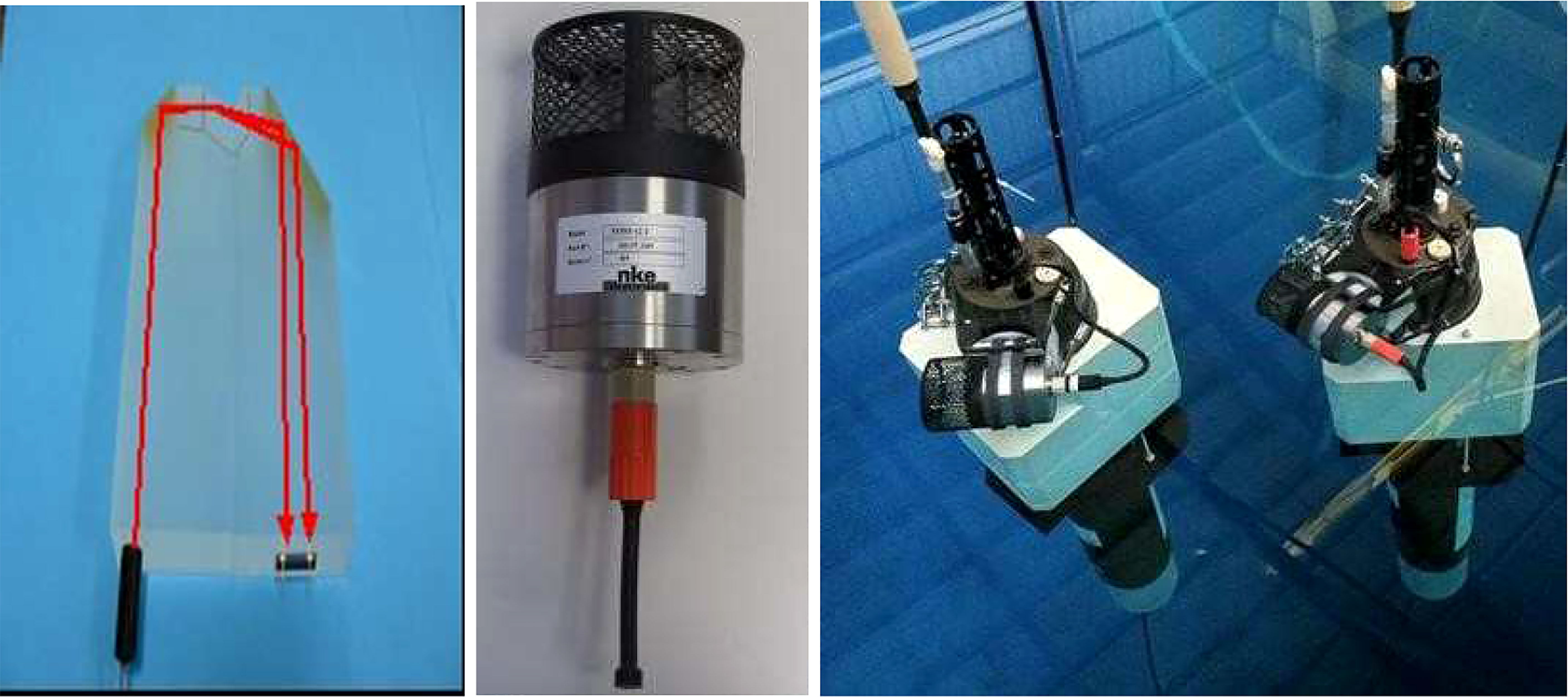
Figure 1 On the left, the principle of a V-block refractometer. In the middle, photo of the NOSS V-block refractometer. On the right, photo of the NOSS on PROVOR Argo profilers.

The floats carrying the refractometers were tested at sea in 2015. The first profile at 1,000 m showed promising results, with deviations inferior to ± 0.03 g kg^-1 when compared to salinity values obtained from colocated CTD casts and the TEOS-10. However, the 1,500 and 2,000 m deep profiles showed larger non-linear discrepancies due to pressure effects on mirrors. To date, work on a new reflection system is still underway to address this issue.

In 2021, a solution was published to improve the resolution of a V-block refractometer by adding a Fabry-Perot cavity at the output of the prisms (Li et al., 2021). This paper demonstrates the possibility of enhancing the resolution of measurement of similar instruments to 1.4 x 10^-8 in the laboratory, but no ideas were given on how to make them usable at sea.

In Seaver, 1985 had already described the principle of a refractometer based on total reflection in U.S. patent application nos. 719, 346 and 719, 399. The instrument was based on a prism illuminated by a white light source at a fixed angle of refraction with a spectrograph as a detector (Seaver, 1987), and suggested the possibility of making in-situ R.I. determinations to better than 1 x 10^-5 by measuring wavelength extinction.

The principle was taken up by Chen et al., 2018 but with a simple laser diode emitting at 635 nm and a 1600 x 1200 pixel CCD camera to detect the reflected light (Figure 2). With this sensor, they achieved a resolution of 1.17 x 10^-5 and a repeatability of ± 6 x 10^-5 (at 2σ) for the R.I. determination. The sensor was field-tested in the eastern part of the Yangtze estuary, where turbidity is important, and the results for salinity obtained with it showed good agreement with the values of the quantity recorded by a SBE 37-SI CTD (correlation coefficient of 0.994).

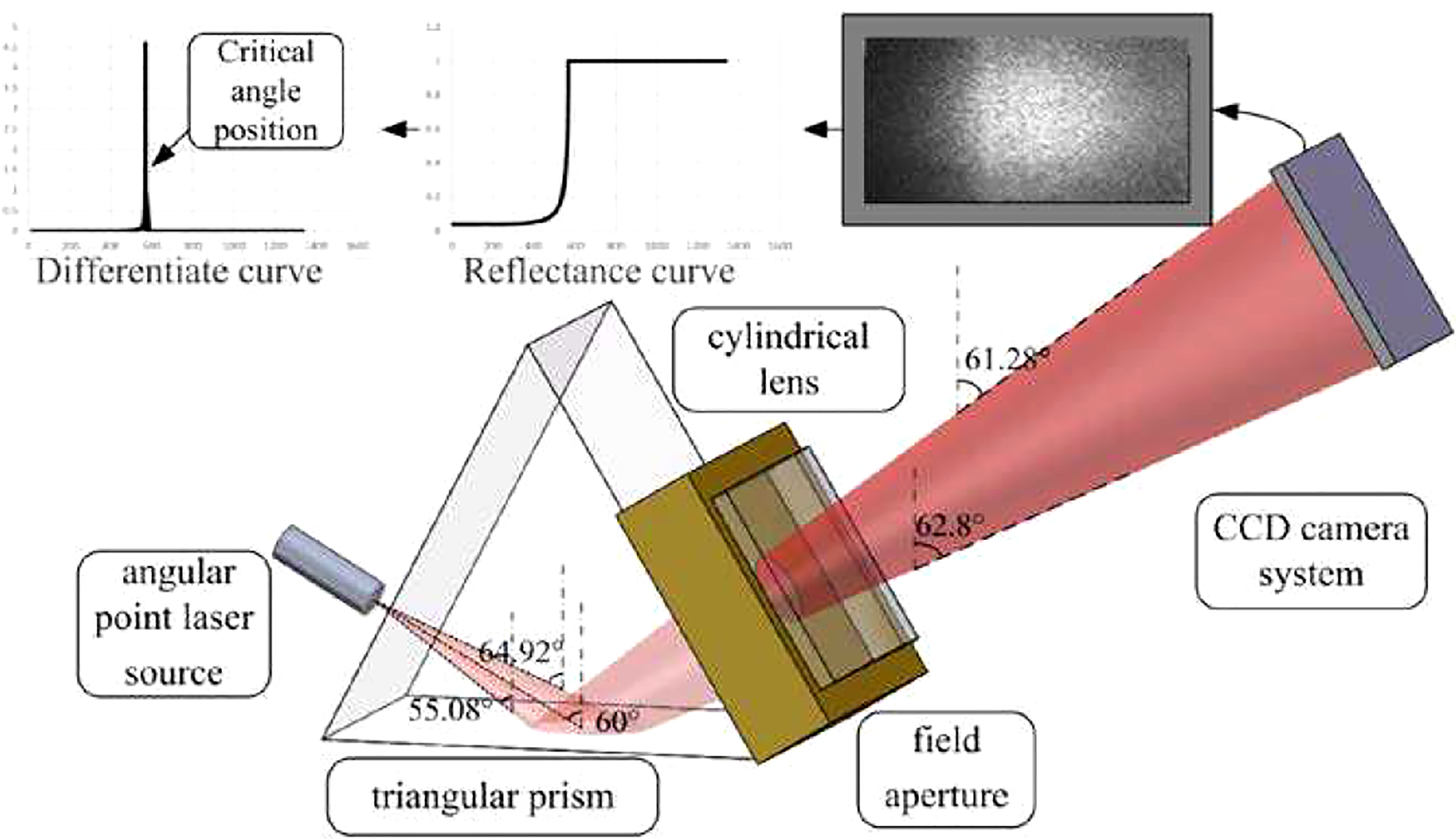
Figure 2 Principle of a refractometer based on total reflection (from Chen et al., 2018).

The advantage of such a configuration is its simplicity, and the fact that the light path is completely inside the sensor thereby reducing the effect of turbidity. The drawback is that the measurement is made in the thermal limit layer, reducing the accuracy of profiles and the usability of the device.

More recently, Jing et al. (2022) describes a comparable instrument but one which is developed on a monolithic chip from an epitaxial structure containing InGaN/GaN multi-quantum-wells that takes the in-situ salinity sensor to the chip-scale. The total reflection is made in a sapphire glass deposited on a n-GaN layer. According to the relationship q_c = arcsin(n_w/n_g), the critical angle q_c widens when the refractive index n_w of the water increases, assuming that the refractive index n_g of the glass remains constant. More light is then emitted out of the chip and less light is detected by the integrated photodetector.

Although this set-up suffers from some flaws that affect the accuracy of the measurements, it is probably a real breakthrough in salinity measurement. The maximal resolution of the instrument is given as 1 x 10^-3 in salinity. Its repeatability is not quantified but seems reasonably good. In the publication, a solution to protect the glass from fouling is also provided. It is based on an ultra-thin mono-layer coating of polyglycerol liner which imparts bio-inert and antifouling properties to the glass both in vitro and in vivo’ (Jing et al., 2022). The effect of this coating is demonstrated to be efficient, and it only produces a simple shift of the device’s linear calibration curve.

Interferometric techniques to measure refractive index

Interferometric techniques permit better resolutions as they are based on measurements of wave phase differences. These differences can be obtained with two waves or more. Two-wave techniques provide differential measurements facilitating the attenuation of some instrumental errors.

Various classical interferometer set-ups have been evaluated in the laboratory. Mahrt and Kroebel, 1984, used a two-wave Mach Zehnder assembly with a thermostatically controlled cell in each arm to compare a salt solution to a reference water. With a resolution of the fringe count of 1/100^th of a fringe, they estimated that they could determine salinity to better than 4 x 10^-4. This instrument from the Institute of Applied Physics (Kiel, Germany) could have been used to make accurate measurements of the R.I. of seawater at different salinities and temperatures, but these measurements were never made. The same technique was used by Lu and Worek, 1993 to determine the R.I. of salt-water solutions.

Rusby, 1966, tested a two-wave Jamin configuration to measure the R.I. of Standard Seawater at 546.227 nm in the ranges of 30.9 - 38.8 g kg^-1 in salinity and 15 - 30°C in temperature. He obtained a standard deviation of 0.0055 g kg^-1 in salinity. In the Jamin configuration, the beam splitting is done on the back side of a blade with a semi-reflective entrance face. In 1997, Vlasov and Kostianoy (Seaver et al. 1993) used this configuration combined with a Michelson one to make an instrument called Lamina-2, calibrated in the laboratory and used at sea to make R.I. profiles down to a depth of 400 m (see Seaver et al., 1997). The instrument used a reference cell containing pure water traversed by the reference beam, with the other beam passing through the seawater. The phase measurement was made after a heterodyne modulation with a resolution of 1/32 of a fringe, which corresponds in terms of the R.I. to about 1 x 10^-6. The device, temperature-compensated and with a low sensitivity to vibrations, was the size of a CTD profiler: ≈ 1 m long and 20 cm in diameter, with temperature and salinity measurements calibrated to ± 0.04°C and ± 0.005 g kg^-1, respectively.

Stanley, 1971, published an article about seawater R.I. measurements made with a compressible multi-wave Fabry-Perot (FP) interferometer. Mirrors allowing multiple reflections were placed on both sides of a cylindrical cavity which could be pressurized. The diameter of the cavity was 5 mm and its length was about 3 mm. Measurements were performed on Standard Seawater with the nominal salinity of 35 g kg^-1 at wavelengths of 501.7 and 632.8 nm in the temperature and pressure ranges of 0 - 30°C and 0 – 13,880 dbar. He obtained a standard deviation of 2 x 10^-5 and an experimental error of ± 6 x 10^-5 for the R.I. measurements. These data were also used later by Millard and Seaver to build their algorithm. Andersson et al., 1987, constructed a compressible multi-wave FP interferometer of the same kind to measure the refractive index of air under pressure. More recently, the interferometric principle of FP has been developed with optical fibers (see § 3.4).

Interferometric fringes can also be produced by illuminating a capillary with a coherent light source. This technique was first developed to improve detection in high-performance liquid chromatography (HPLC) equipment. It was used by Le Menn and Lotrian, 2001 in the form of a cube-capillary. The cube form bestows a good resistance to pressure effects. When illuminated by transmitted light, the cube-capillary behaves like a two-wave interferometer. An uncertainty of 1 x 10^-6 can be obtained for the R.I. measurement, but over a low range of R.I. variation (1.5 x 10^-4). To improve this result, it would be necessary to increase the capillary diameter and to work on a more complex technique of phase measurement (Le Menn, 2000).

In order to develop a new optical method to measure the refractive index of seawater having longterm stability, Asakawa et al. (2010) used a heterodyne Michelson interferometer. The laboratory prototype was tested on pure and saline water (3 ‰). The result coincided with the theoretically expected value within an accuracy of ± 1.6×10^-5.

Like refractometers, in the last years, interferometers too have been the subject of research in the race to build monolithic devices. Ahmadi et al., 2016, (a Finnish team) described a polymer slot waveguide Young’s refractometer coated with a bilayer of Al₂O₃/TiO₂ that is also a two-wave interferometer (Figure 3). Al₂O₃ or Alumina is a compound with interesting properties: it is an electrical insulator and a thermal conductor. The feasibility of this device has been investigated at the 975 nm wavelength, and its performances have been tested with an ethanol-water solution at different concentrations. The smallest phase shift measured is 0.007 ± 0.003 rad, corresponding to a resolution of 1.07 x 10^-6 in R.I., with a very small sensing length of only 0.8 mm. The measurement range of this low-cost sensor is not given. A question remains regarding the small size of the sensor’s detection parts and its effectiveness in measuring natural seawater loaded with particles.

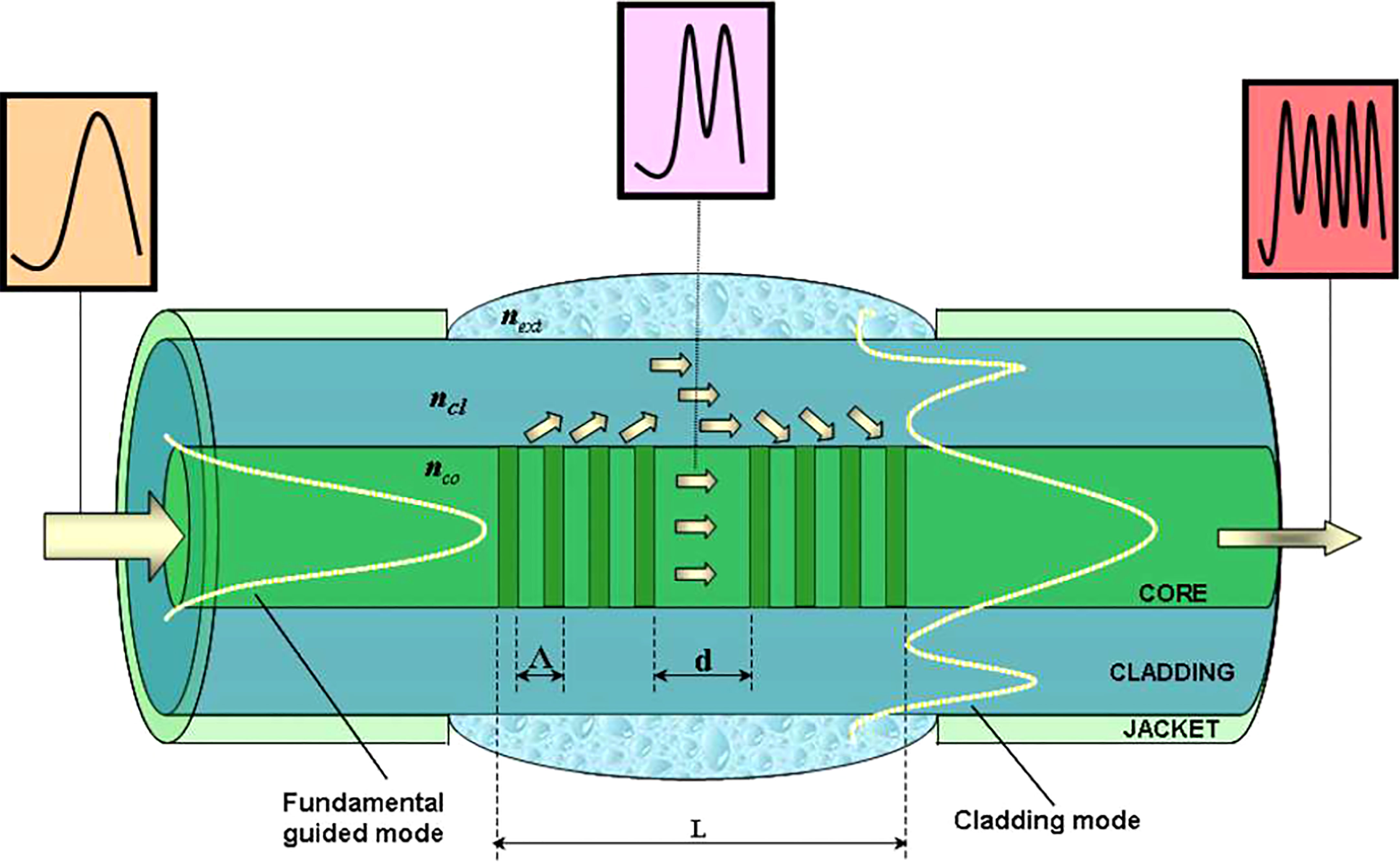
Figure 3 Scheme of an in-fiber Mach-Zehnder interferometer based on two cascaded LPFGs. The spectral shape of light is represented before the first grating and at the output of the second grating (from Possetti et al., 2009).

The Mach-Zehnder (MZ) configuration was also the object of a numerical study by Mishra et al. (2022) to make a silicon-on-insulator platform. Two different schemes of MZ-based electrolytic sensors were investigated using the Finite Difference Eigenmode method. The authors concluded that a rib waveguide-based sensor demonstrates greater sensitivity when compared to a strip waveguide-based sensor, but it is difficult to say much about the potential of this technology based only on their study.

Other interferometer principles have been studied in the effort to make low-cost R.I. measurements. Ma et al., 2017, published a paper about a polymer fiber Fizeau interferometer with a highly hygroscopic polymer directly coated on the end faces of two fibers that helped to measure temperature and humidity variations also. The resolution and the range of the interferometer in terms of the R.I. were not given, but the technique could perhaps be adapted to measure seawater salinity.

The Mach-Zehnder configuration has also been used with a polymer waveguide to detect nitroaromatic components (Jiang et al., 2020). Similarly, the FP configuration too has been employed with an optical fiber coated with three different polymers to measure temperature (Salunkhe et al., 2021). However, in both the cases, the resolution and the range in R.I. are not given.

Various techniques based on the use of optical fibers

Optical fibers were utilized to develop a lot of sensing techniques, and some of them have also been employed in the measurement of salinity. In the 80’s and 90’s, they were employed to transmit light to prisms, and to construct refractometers (see for example Mahrt and Waldmann, 1988; Minato et al., 1989, and Zhao and Liao, 2002).

In the 2000s, the use of the fiber Bragg grating (FBG) technique was explored by several researchers. FBGs were components developed in the 90’s to make spectrally selective band filters for telecommunications and sensors (Marrec et al., 2005). A grating is a permanent and periodic modulation of the fiber core refractive index. The modulation is obtained by exposing the fiber to an interference pattern of UV light. The period of the modulation can be long (100 to 500 μm), giving rise to the Long Period Fiber Grating (LPFG), or short (< 1 μm), leading to the Short Period Fiber Grating (SPFG). Several commercial applications of the technology exist to measure temperature and strain. The difficulty lies in avoiding the effect of these two quantities when using the technology to measure other quantities like salinity.

However, Swart, 2004, used a LPFG to make a Michelson interferometer applying the mode coupling method. The phase shift of the device depended on the R.I. of the surrounding medium and its sensitivity was proportional to the probe length. For a 45 mm probe, Swart obtained a temperature sensitivity of 0.35 nm °C^-1. With a period of 9.9 nm for the interference pattern, this gives a sensitivity of 12.7° °C^-1. He also carried out trials with various solutions of glycerine, obtaining a sensitivity of 1571° R.I.U.^-1 in the R.I. range of 1.33 - 1.40. The device’s sensitivity to the surrounding medium is therefore much greater than its sensitivity to temperature. However, it would be necessary to measure variations of 0.0015° to obtain a measurement of 1 x 10^-6 in R.I., which seems hardly realizable, thus making the device unsuitable for oceanographic use.

A wave Bragg Grating was tested by Dai et al., 2006. They found that a change of 4 x 10^-5 for a R.I. around 1.40 led to a shift of 1 pm in the resonance wavelength. Measuring 1 pm is not easy. 4 x 10^-5 also seems to be the resolution limit of this method. Phan Hui et al., 2006, used a micro-structured optical fiber (MOF) with photo-writing Bragg grating. In MOFs, light is guided by total internal reflection. They tried out their sensor in liquids in the R.I. range of 1.33 - 1.39. For a six-hole MOF, they found a resolution of 8 x 10^-4 that could reach 7 x 10^-6 around the more important Bragg resonance shift. These numbers also appear in a publication of Kamikawachi et al. (2007) about the influence of the surrounding refractive index on the thermal and strain sensitivities of cascaded LPFGs. Possetti et al., 2009, published a paper on an in-fiber Mach-Zehnder interferometer made with two LFPGs forming an in-series 7.38 cm long device written in the same optical fiber (Figure 4). They obtained an average sensitivity of - 6.61 pm g^-1 l^-1 with NaCL solutions, corresponding to - 40.8 nm R.I.U.^-1 for concentrations up to 150 g l^-1. Once again, even if this sensor seems able to provide salinity measurements over a large range, its sensitivity and resolution is very low.

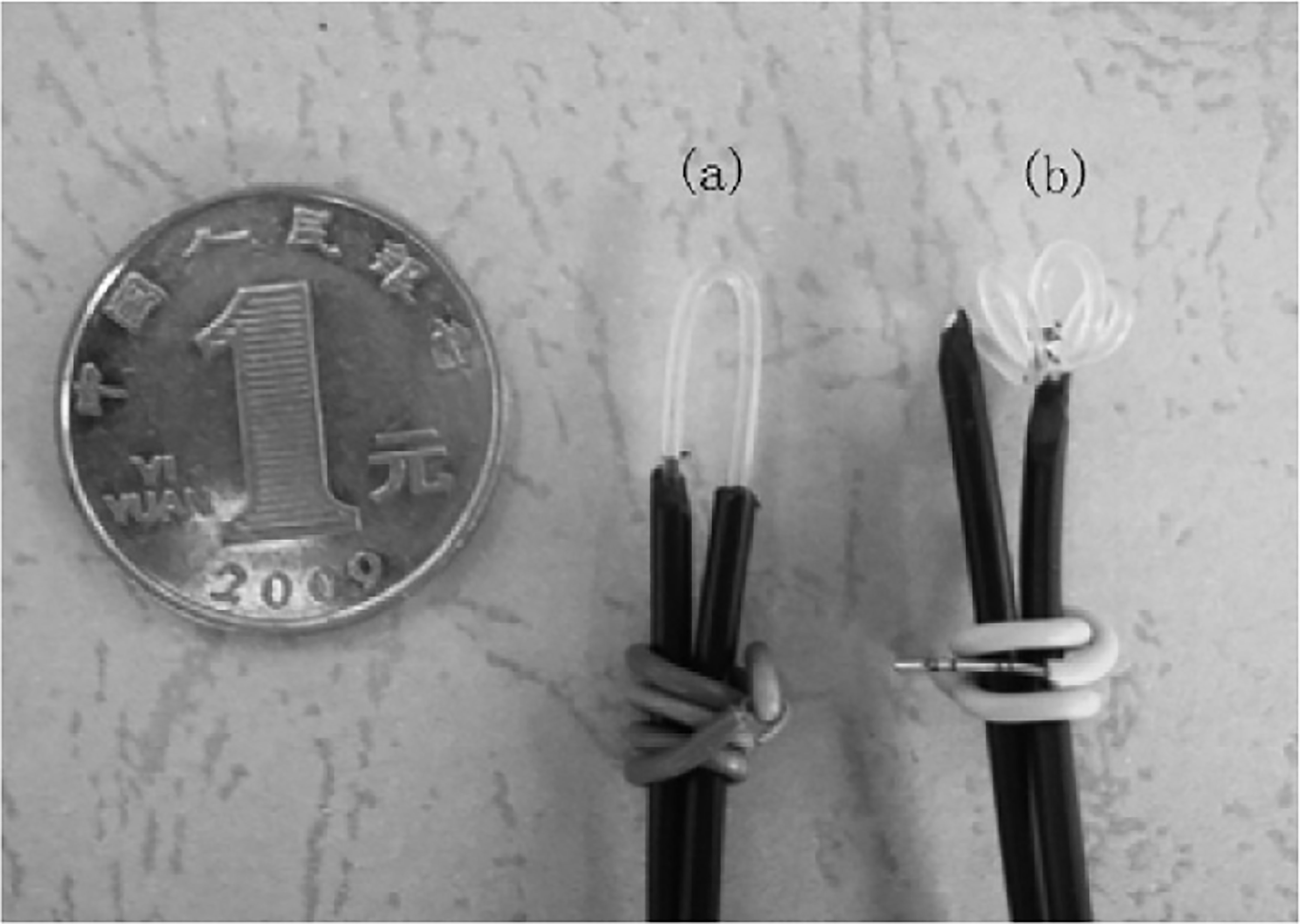
Figure 4 (A) U shaped and (B) spiral shaped plastic optical fibers. (from Wang and Chen, 2012).

In conclusion, various FBG and LFBG techniques have been explored but none of them seem to be capable of providing the R.I. measurement resolution and range required for Oceanography.

Recent advances in various techniques

Over the past 10 years, researchers from China were very active in the development of new solutions to measure the R.I. of seawater, and a lot of recent advances in this field come from researchers of this country. Wang and Chen, 2012, tried to measure salinity with plastic optical fibers, spiral as well as U-shaped, to amplify the intensity of evanescent waves radiated in seawater (Figure 3). This intensity is proportional to salinity, and its variations can be followed by measuring the power of the light at a fiber’s output. With concentrations from 0 to 35%, they obtained sensitivities of 0.42 mV/% for the U-shaped fiber and 0.13 mV/% for the spiral one. 35% being 350 g kg^-1, an instrument able to detect 1 μV would provide a resolution of 0.1 g kg^-1.

In 2017, in order to try and improve the FBG technique, Luo et al. 2017 tested an etched FBG sensor coated with polyimide to detect salinity and temperature simultaneously. By measuring the displacement of the fundamental mode resonance wavelength and thanks to a matrix equation, they obtained sensitivities of 125.92 nm R.I.U.^-1 for the R.I. and 0.0435 nm °C^-1 for the temperature. With an instrument able to detect 1 pm, these make for resolutions of 1.3 x 10^-5 in R.I. and 0.4°C in temperature.

In the same year, several other papers were published about R.I. measurements in liquids. Xu et al., described a device made of a tiny segment of capillary tube inserted between single-mode fibers to form two cascaded FP interferometers. By measuring the intensity and the shift of the resonant wavelength in the reflection spectrum, they were able to determine the R.I. and temperature of the ambient liquid with a sensitivity of 216.37 dB R.I.U.^-1 for R.I. = 1.30. In the 1.3333 – 1.3474 R.I. range, the sensitivity was 133.52 dB R.I.U.^-1. According to the authors, it is possible to measure the intensity with a resolution of 0.01 dB, corresponding to an index resolution of 7.5 x 10^-5, with a Yokogawa AQ6370D laboratory optical spectrum analyzer.

Wang et al. (2017), describe a R.I. sensor based on a linear-cavity dual-wavelength erbium-doped fiber laser capable of making measurements in the short range of 1.3 to 1.335 with a maximal (and not constant) sensitivity of – 273.7 dB R.I.U.^-1, meaning a R.I. resolution of 1.5 x 10^-5. Other authors (Chen et al., 2017) experimented with surface plasmon resonance on a gold film and a dual-frequency laser to make heterodyne interferometric R.I. measurements. Tests carried out on glycerin solutions in the 1.333 – 1.336 R.I. range and comparisons made with an Abbe refractometer showed differences lesser than 2.0 x 10^-5 in R.I. with an uncertainty< 3.0 x 10^-5.

In addition to Chen et al. (2018), another method uses a fiber laser intracavity loss modulation has been developed by Xu et al. (2019). The authors considered the detection limit of their sensor to be 0.0023 g kg^-1, taking into account errors related to the stability and resolution of the photodetector as well as the cross-sensitivity with temperature.

The FBG structure was tested again by Yin et al., 2019 but this time associated with a cascaded dual-wavelength fiber laser and a single-mode-no-core-hollow-core-no-core-single-mode (SNHNS) structure (Figure 5). In this assembly, the output power and the wavelength shift were measured to give a high sensitivity of – 367.9 dB R.I.U.^-1 in the 1.334 – 1.384 R.I. range. With a high-resolution spectrum analyzer capable of reading down to a level of 0.1 dB, this would mean 3 x 10^-4 in R.I.U. - which is still not good enough to meet oceanographic requirements. Moreover, the assembly is sensitive to the changes in temperature caused by the variability of the laser output power, which leads to uncertainties of 0.22 dB °C^-1.

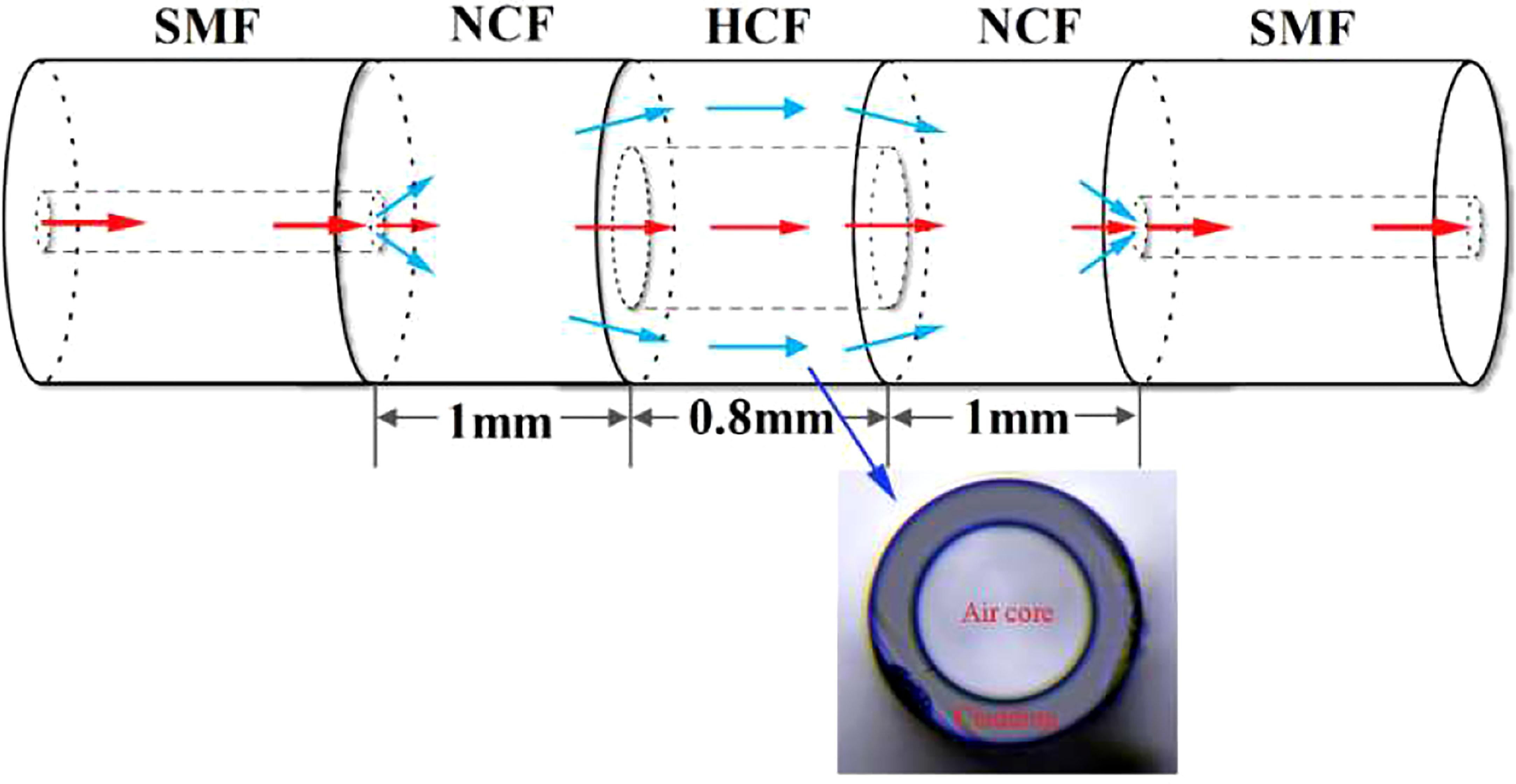
Figure 5 Schematic diagram of a SNHNS structure and picture of a cross-section of the hollow-core fiber (from Yin et al., 2019).

In 2019, a splicing point tapered fiber Mach-Zehnder interferometer was also tested by Liu et al., 2019 (Figure 6). The device allowed the simultaneous measurement of temperature and salinity with sensitivities of – 994.83 pm °C^-1 and 290.47 pm (g kg^-1)^-1. With a high-resolution reading instrument of 1 pm, this could provide a resolution of 0.003 g kg^-1, but the authors didn’t report their limit of detection (LOD). Besides, the assembly was encapsulated to avoid strain and pressure effects, and it presented a short response time of 33 ms. Furthermore, while the repeatability was tested, it was not quantified accurately. Han et al., 2020, tested a novel fiber-interface directional waveguide coupler inscribed on the surface of a coreless fiber by a femtosecond laser, achieving a sensitivity of 8249 nm R.I.U.^-1, but over a range of the R.I. outside that of seawater: 1.44 – 1.45.

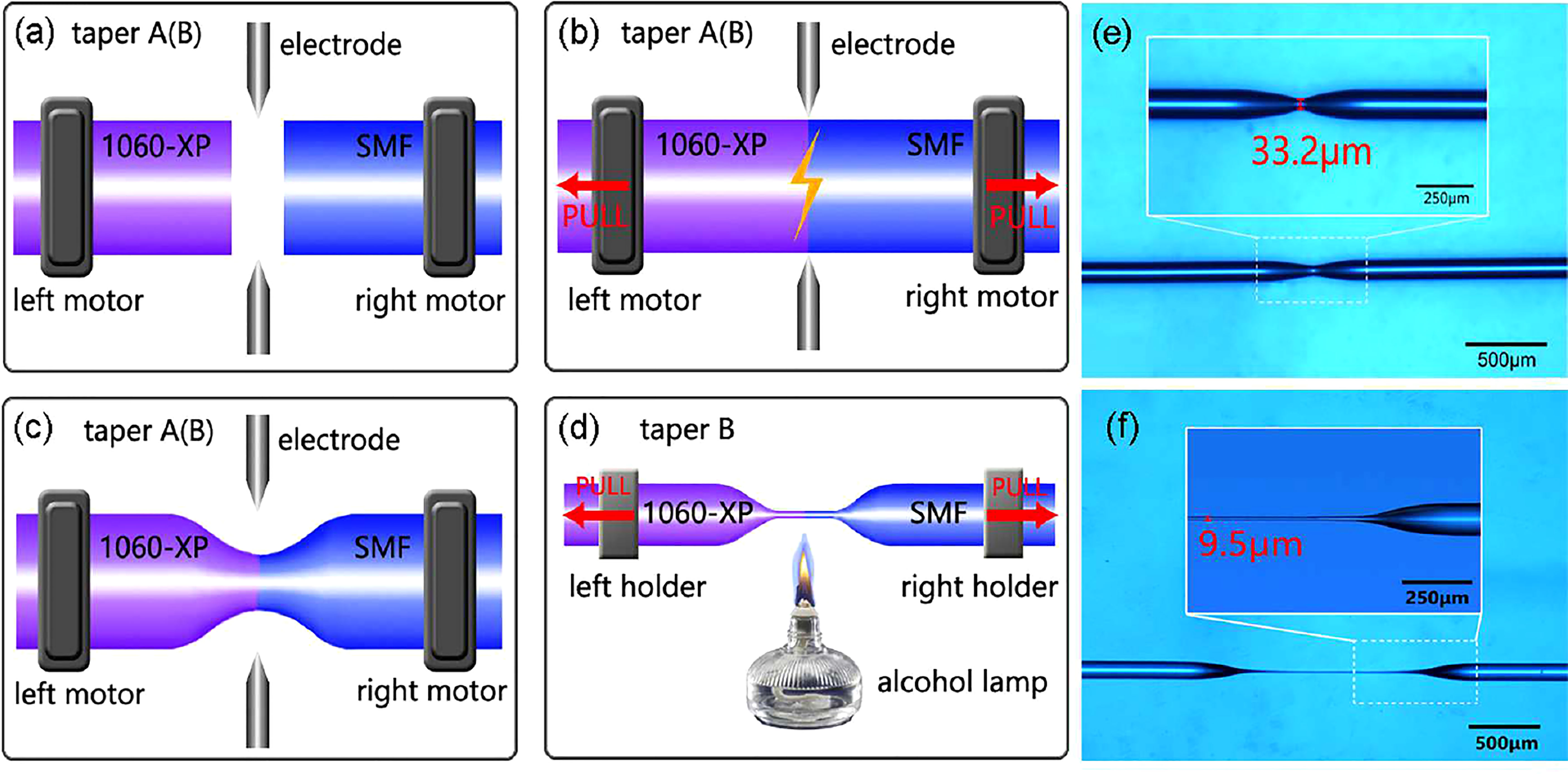
Figure 6 Representation of the fabrication steps of tapers to form a Mach-Zehnder interferometer: figures 6(a) - 2(c) show the fabrication steps of taper A or B. (d) Further tapering on taper B by alcohol lamp heating. Optical micrographs of the completed (e) taper A and (f) taper B (from Liu et al., 2019).

It should be noted that in 2019, a setup based on a fibered FP structure was published by Flores et al. 2019 from the Masdar City Campus in the United Arab Emirates. This sensor consisted of FP optical cavities, formed by chemical etching and fusion splicing, onto which microfluidic channels were milled by a focused ion beam. A configuration based on the Vernier effect composed of a sensing and a reference cavity was reported for salinity and temperature sensing. The sensor was tested in the small R.I. range of 1.3176 – 1.3212 where it showed a high sensitivity of 1150 ± 24 nm R.I.U.^-1, but the authors give the 3-sigma LOD as 3.6 x 10^-3 M or 0.21 g l^-1 for NaCl. With δρ = 0.75179 x δS (Woosley et al., 2014), this translates into a poor resolution of 0.28 g kg^-1 in salinity. Another kind of FP sensor was tested by Xia et al. 2021 to measure high temperatures and strain. It consists of a silica-cavity intrinsic FP interferometer (IFPI) cascading an air-cavity extrinsic FP interferometer (EFPI). The sensitivity of the assembly seems to be low: 16.12 nm °C^-1.

Niu et al., 2020, also tested a micro-cavity structure, but it was open and in a Mach-Zehnder configuration. They obtained an interesting sensitivity of – 2953.4 nm R.I.U.^-1 with it, corresponding to an enhanced detection limit of 5.9 x 10^-6 R.I.U. with a high spectral quality factor of 2.2 x 10¹⁰, but in the low R.I. range of 1.333 to 1.334.

Surface Plasmon Resonance (SPR) has also been tested by Zhao et al. (2019) in a classical form (Figure 7), and in the form of an optical quantum sensor dependent on a tapered hetero-core structure coated with a 50 nm gold film (Zhao et al., 2020). The input source is a single photon used for exciting surface plasmon polaritons at the interface between the metal and the seawater. The utilization of a statistical analysis method helped attain a resolution of 0.0016 g kg^-1. The measurement range was not given. According to the authors, the technique was promising and could pave the way to the development of high-resolution and high-sensitivity sensors.

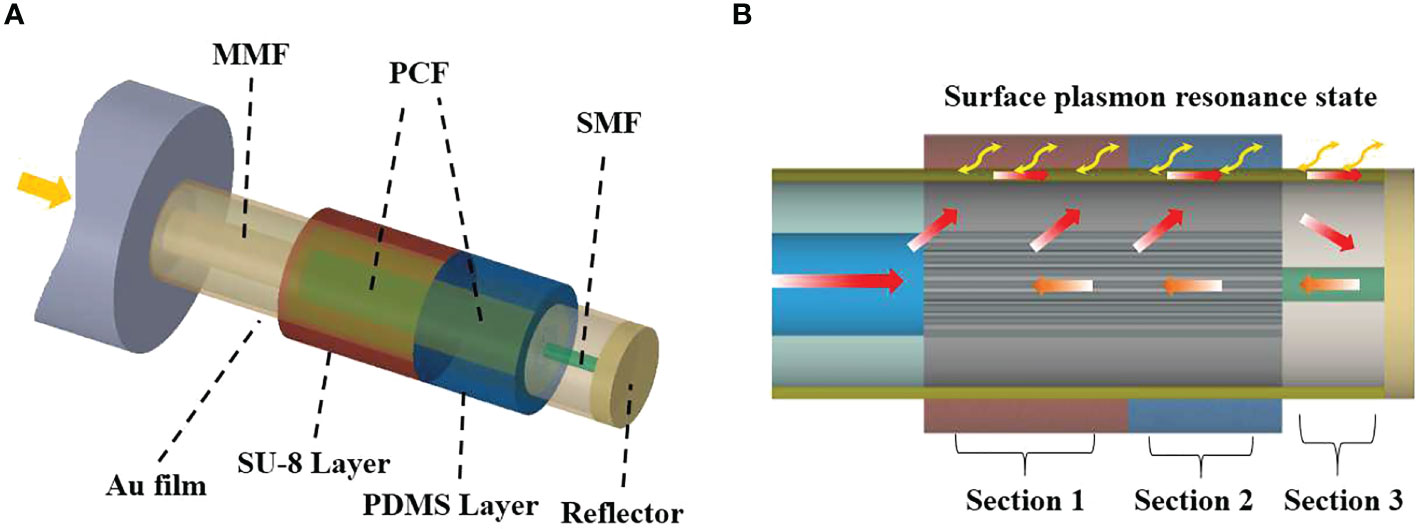
Figure 7 Schematic of the SPR sensing principle tested by Zhao et al, 2019. It is composed of a combined reflective structure with multi-mode fiber (MMF), photonic crystal fiber (PCF) and single-mode fiber (SMF) (A). (B), illustration of the SPR effect (from Zhao et al, 2019).

The SPR technique was experimented again by Yang et al., 2021 using a micro-structured optical fiber with the sensing channel coated with indium tin oxide and gold. While the R.I. range is interesting (1.33 – 1.39), the sensitivity to salinity seems to be insufficient: 0.45 nm (g kg^-1)^-1. It would be necessary to measure 0.5 pm in order to detect 1 x 10^-3 g kg^-1, which is very low.

In 2022, Zhiyong et al., 2022 published a paper on a simulation of a twin-core photonic crystal fiber sensor with air holes arranged in a hexagonal pattern executed with the finite element method. On one side of the plane, a gold film is deposited for R.I. measurement while a gold film and polydimethylsiloxane are deposited for temperature measurement on the other side, creating a multiparameter SPR sensor. They found the maximum spectral sensitivity of the sensor to be 20 000 nm R.I.U.^-1 and 9.2 nm °C⁻¹, respectively, when the R.I. of the liquid is in the range of 1.36 – 1.42 and the temperature in the 0°C – 50°C interval. These ranges are compatible with oceanographic needs, and the sensitivity would allow a resolution of 1 x 10^-6 in R.I. (0.0059 g kg^-1) if the resolution on the wavelength measurements was 0.02 nm, but these are numbers which are results of a simulation.

A similar sensitivity (- 19844.67 nm R.I.U.^-1) was obtained in 2022 by Jiang et al. with a hybrid fiber interferometer, consisting of a fiber Sagnac interferometer (FSI), a closed-cavity Fabry-Perot interferometer (FPI), and an open-cavity FPI which served to generate a combined-Vernier-effect. The optical Vernier effect is similar to the method used in calipers to improve the reading resolution. In optics, the Vernier effect acts as a mechanism to suppress spectral modes (resonance peaks in a spectrum) and narrow the linewidth of fiber lasers. In Jiang et al. (2022), two Vernier effects are used to separately detect temperature and R.I. variations. It is perhaps a promising technique, but also one that is complex and has been tested only in the 1.333 to 1.339 R.I. range in the laboratory.

Other fiber-optic measurement principles have also been tested recently by Chinese teams - a tapered dual-core As₂Se₃-PMMA (polymethyl methacrylate) hybrid fiber (Wang et al., 2021) and a femtosecond laser-inscribed fiber-optic sensor (Zhao et al., 2022) - but the sensitivities obtained are low.

To conclude on these recent developments, it seems that most of the experimented fiber-optic techniques offer sensitivities, resolutions and measurement ranges that are not good enough currently to meet oceanographic requirements, but recent publications show that improvements are still possible.

Two other promising developments that have been published and are worthy of mention are described below. The first is also based on fiber-optic using. Atkins et al., 2002, deposited a patent for a single mode fiber-optic evanescent wave refractometer. The plastic buffer of two single mode fibers is removed and they are fused in a furnace. The operation is performed under constant tension to elongate the fibers. The light transmitted through one fiber, is coupled to the other fiber as well. Since the cladding of the fibers has been removed, the surrounding medium becomes the new cladding and its refractive index modulates the coupling ratio. If this coupler is fixed in a stable housing, the coupling ratio of power α in the second fiber is given by:

$\alpha =\frac{I_2}{I_1+I_2}$ (6),

where I₁ and I₂ are the intensities measured at the outputs of the fibers (see Figure 8). α depends only on the wavelength of the laser and on the R.I. of the surrounding medium averaged over a one-optical-wavelength-thick cylinder. This means that the sensitivity increases with the wavelength, but the effect of source intensity variations (with temperature for example) are attenuated by the ratio of relation (6).

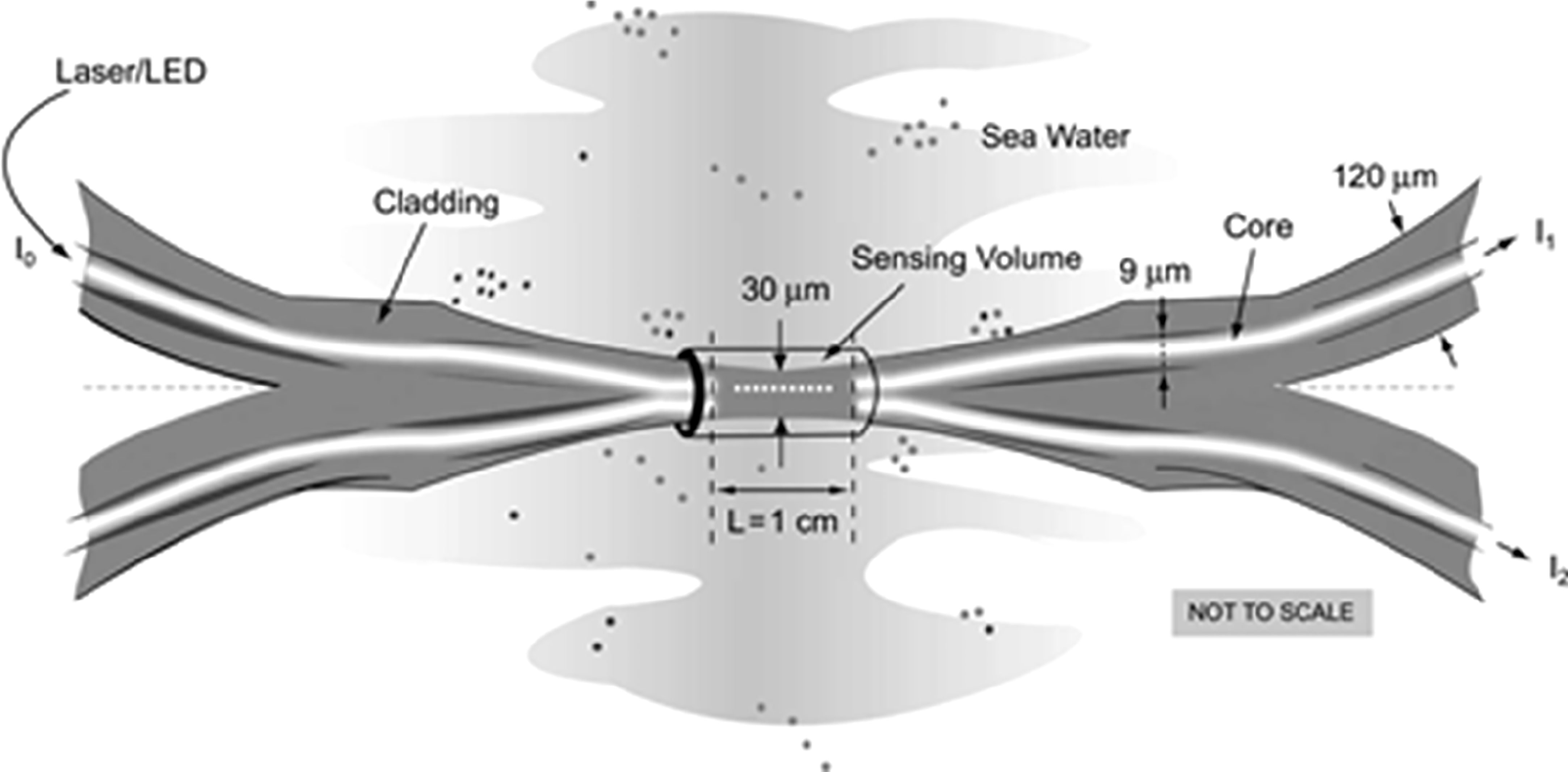
Figure 8 Schematic of the fused fibers with the cladding removed in the sensing area from Alford et al., 2006. The input intensity I₀ and the output intensities I₁ and I₂ are represented.

The above patent was the focus of a sensor development venture and a publication (Alford et al., 2006) concerning an ocean refractometer capable of resolving millimeter-scale turbulent density fluctuations. The obtained sensitivity was 0.0162 W (g kg^-1)^-1, allowing resolutions superior than those of CTDs: 7.8 x 10^-9 in R.I., 7.8 x 10^-5 in temperature and 4.4 x 10^-5 in salinity. The signal was digitized at 50 Hz with a 16-bit converter. The sensor was tested to a depth of just 160 m to measure microstructure, but the probe sensed turbulent velocity in addition to refractive index because the fiber was not sufficiently immobilized on its support. The effect of pressure and strain on the fibers was not reported. Despite the performance reported, no commercial product was developed.

Another patent was filed by Kapit et al., 2016 for a n-wavelength interrogation system and method for multiple wavelength interferometers. It is based on two fiber optic couplers, one acting as a Michelson interferometer and the other one as a Fabry-Perot interferometer. The assembly is followed by a grating and a 16-element photodiode array to measure the spectral intensity of wavelengths emitted by a superluminescent diode centered at 1061 nm with a bandwidth of 30 nm (Figure 9). The 16 signals can be digitized using a 20-bit ADC at a rate of 1 kHz. These multiple wavelengths allow the determination of the directions of scrolling of fringes and an accurate measurement of phase shifts. The instrument was a research project entitled ‘An Optical Interferometer for the Measurement of Absolute Salinity’, funded by the National Science Foundation (https://www.nsf.gov/awardsearch/showAward?AWD_ID=1536781#2). The report of the outcomes of the project states the following: “Over the course of the project we designed, fabricated, and tested the sensor at Woods Hole Oceanographic Institution, and it was successfully deployed during a sea-trial near Monterrey Bay, CA to a depth of 1020 meters. The sensor’s resolution as characterized through lab tests and at sea was exceptional. Overall, it was able to detect density changes as small as 0.00007 kg m^-3 for a sample size of 1 mm³ and at a sampling rate of 500 Hz. These figures make the measurement technique the most sensitive salinity/density detection method to date. Furthermore, its accuracy during the sea-trial showed experimental error below the best currently available models for seawater’s refractive index.

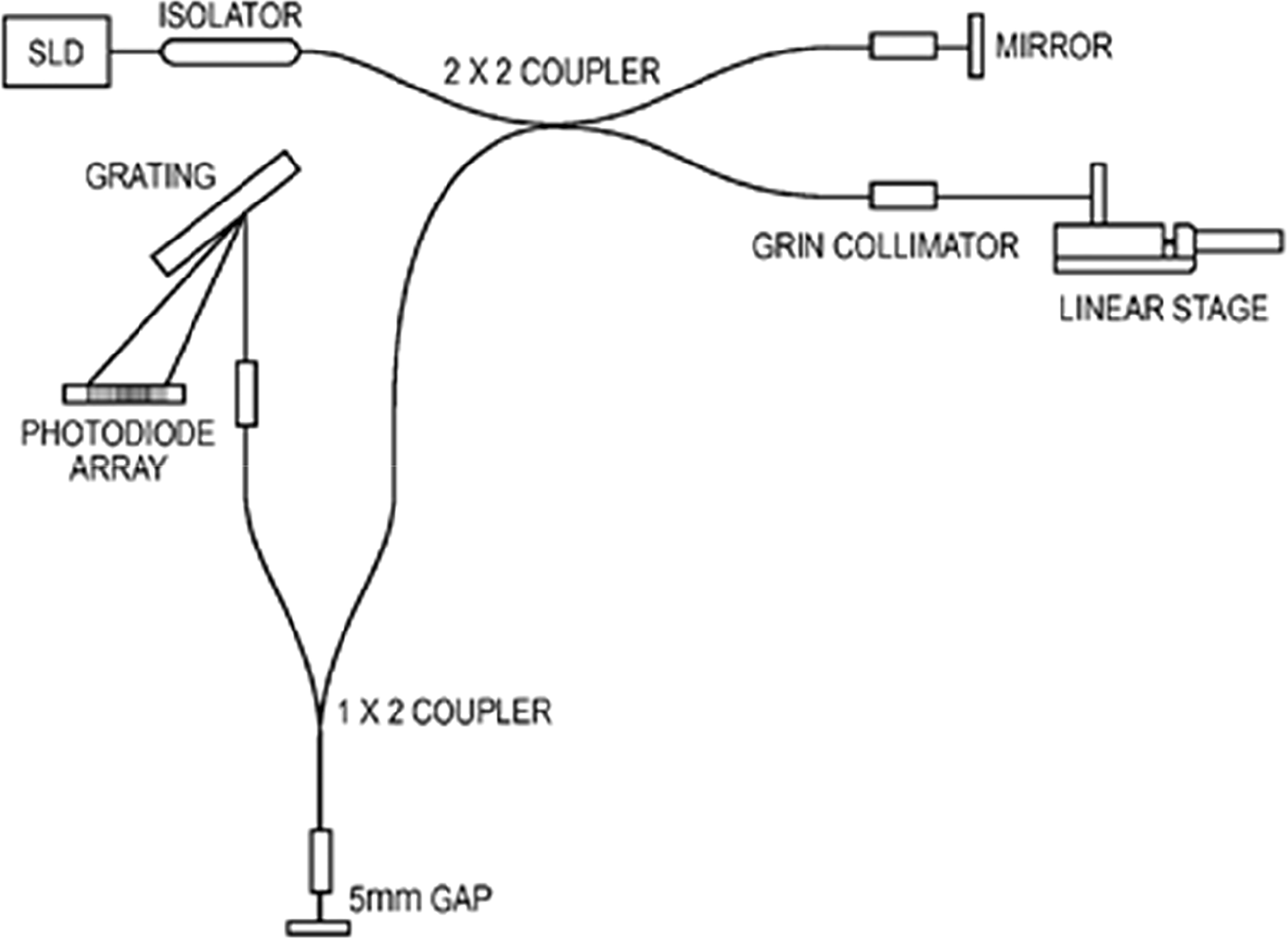
Figure 9 Scheme of the interferometer patented by Kapit et al. (2016).

The overall form factor is comparable to existing oceanographic sensors and it has proven to be surprisingly robust, requiring no significant maintenance or servicing during its lifetime. We have been awarded a patent on the technology, and through future work we intend to pursue commercialization.” Despite this encouraging conclusion, which is dated 01/20/2021, no other publication has ensued and no instrument has been commercialized so far.

The other promising development is described in a paper written by Uchida et al., 2019. It is based on a seawater density measuring cell made from synthetic silicate glass the authors themselves developed, coupled with a commercially available thickness meter from Keyence Co. (model SI-F80). The cell is composed of a beam splitter that divides the beam coming from a super-luminescent diode centered at 820 nm into two separate beams: one is for reference and the other passes through the test sample (Figure 10). Both the secondary beams are reflected by mirrors and combined by the beam splitter to make interferences. The thickness meter contains a spectroscope that splits the broadband interference light into its different wavelengths allowing the difference between the two optical path lengths to be determined thanks to a waveform analysis performed by the meter itself.

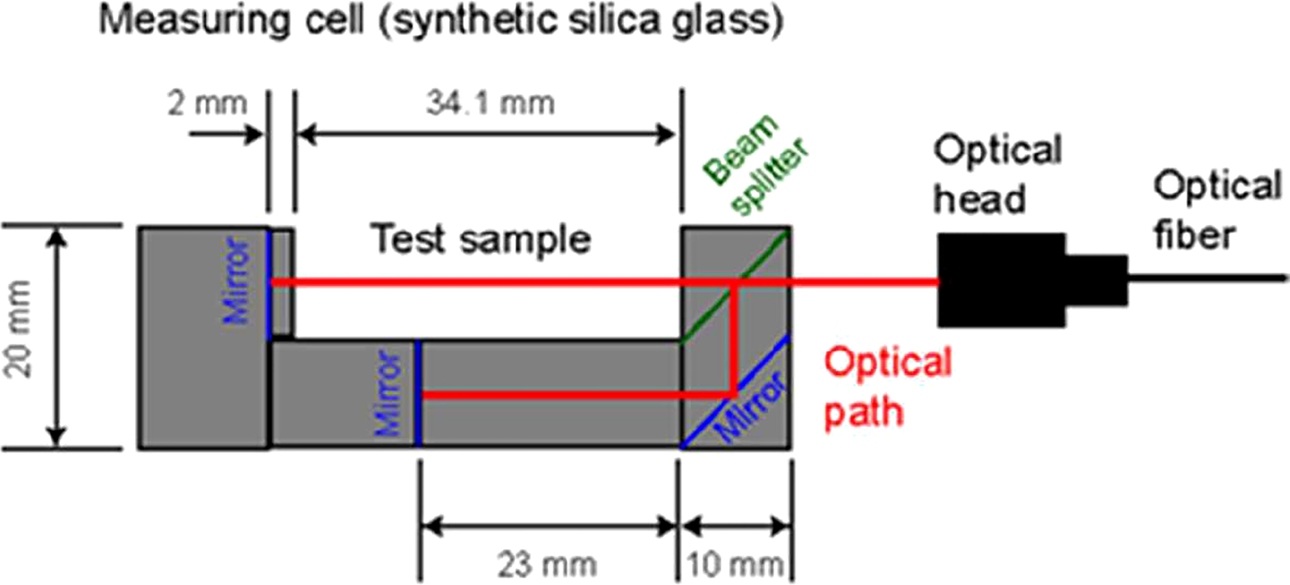
Figure 10 Scheme of the measuring cell (from Uchida et al., 2019).

The apparatus was calibrated in the laboratory with pure water and seawater by varying temperature. The calibration involved fitting density ρ predicted from the TEOS-10 equations to a complex polynomial in sensor output δx, temperature T and pressure P with a least-squares method:

where C₀ to C₁₈ are coefficients to retrieve. Nothing is said about how pressure variations were generated to obtain coefficients C₁₅ to C₁₈ at constant temperature. The effects of temperature on the wavelength are also ignored. The resolutions obtained are impressive: 6 x 10^-5 kg m^-3 at 35 g kg^-1 with changing temperature, 1.2 x 10^-4 kg m^-3 - equivalent to 1.5 x 10^-4 g kg^-1 in salinity - with changing salinity at 1°C, and 1.0 x 10^-4 kg m^-3 at 35 g kg^-1 with changing pressure. The range of measurement for salinity is 0 – 120 g kg^-1. The sampling frequency is 5 kHz for a practical resolution of 0.01 kg m^-3 or 1.2 Hz for a practical resolution of 0.0001 kg m^-3.

However, equation (7) accounts for seawater density variations but also for all the effects of temperature and pressure on the sensor (dilatations, changes in geometry, changes of glass refractive index) and it is also dependent on the accuracy of the TEOS-10. The variability of the results obtained with respect to corresponding TEOS-10 densities has a standard deviation of 0.0011 kg m^-3 and a residual of 0.0035 kg m^-3 typically. Furthermore, the equation cannot be used for making measurements of R.I. and density directly, and most importantly, doesn’t allow the determination or retrieval of S_A values.

The sensor has been tested at sea down to a depth of 6000 m, giving standard deviations of 4 x10^-4 kg m^-3 for pressures > 20 MPa and 0.0038 kg m^-3 for pressures< 20 MPa. However, it cannot be used on profiling floats because of its weight and size: 14 kg and 21 x 50 cm, respectively. Despite these few defects, this instrument constitutes a great advance in the measurement of density by an optical technique.

Discussion

Measuring or estimating the Absolute Salinity or S_A is a requirement of the TEOS-10 to calculate the thermophysical properties of seawater, and the explicit needs of oceanographers in this respect are the following:

− to determine salinity to the best with an accuracy of 0.002 in Practical Salinity (PSS-78), although for example, coastal applications or satellite measurement validations require lower accuracies.

− To measure the real and local amount of components consistent in sea water and also to determine correctly the sea water density, which is a key state variable for all process that impacted by ocean physics.; recent work reveals that an accuracy on the order of 0.001 - 0.002 g kg^-1 is mandatory for the deep Ocean.

It appears that:

− even though climate studies are based on statistics and a large number of observations, it appears that current techniques are neither sufficient nor satisfactorily effective to assess density and S_A properly;

− making progress in density and S_A measurements is mandatory to improve our understanding of ocean dynamics, biogeochemistry and biology (diffusion into cells and impact on abundance);

− while electrical techniques continue to provide more than 97% of seawater salinity observations and seawater conductivity sensors can be calibrated to a few μS cm^-1, the systematic or random errors introduced by non-electrical constituents present during the measurement of the salinity with these are difficult to assess;

− while electrical techniques are well-adapted for in situ oceanographic measurement, optical or acoustical techniques remain options to explore to advance measurement capabilities for the density and S_A of seawater.

As the speed of sound is inversely proportional to density and directly related to S_A, temperature and pressure, it could be used to measure S_A. Sound velocity sensors are generally low cost, reliable and robust. But, to be able to satisfy the oceanographer’s needs, the measurement of sound velocity needs to be 3 to 60 times better than what it is currently for laboratory instruments and in situ sound velocimeters respectively. Sound velocity sensors for measuring S_A would also need oscillators with greater long-term stability and further studies directed toward understanding and compensating for diffraction effects, if such compensations are possible at all in the first place. The lack of high-quality measurements to establish polynomials relating S_A to the temperature, the pressure and the sound velocity are a further drawback.

The refractive index is an ideal variable to assess the amount of salt in seawater because of its strong link to the density and composition of the medium. It is sensible to the whole dissolved content, but not to suspended matter which just affects the shape and the intensity of optical beams, the limit being fixed by the wavelength used. An empirical relationship exists (Millard & Seaver, 1990) to quantify the variations of the refractive index as a function of temperature, salinity and pressure, but its uncertainty with respect to pressure must be improved if it is to meet oceanographic requirements. Many innovative instruments have been developed to measure the refractive index since the 1990s but none of them have proved completely suitable for in-situ use to date, though some have come quite close.

Optical fibers present the advantages of small size and light weight, and therefore short thermal response times. FBG and LFBG techniques have been explored in several forms but all of them seem to be unable to achieve the resolution and range of measurement required for Oceanography so far. On the other hand, some simple refractometry and interferometry techniques have given good results. Jing et al. (2022) has proven that it is possible to make small monolithic chips from an epitaxial structure and obtain a resolution close to 1 x 10^-3 in the measurement of salinity with them. While their set-up suffers from some flaws that affect the accuracy of the measurements, it is probably a real breakthrough. Other refractometers, like the V-block refractometer of Malarde et al. (2009) or the total reflection refractometer (Chen et al., 2018), have already been tested at sea. The V-block refractometer suffers from some problems relating to high pressure which are being solved whereas the total reflection refractometer (which was not tested to great depths) does not possess sufficient resolution. For these instruments, progress is possible if investments are made.

Interferometry techniques have demonstrated the possibility of obtaining high resolutions, and one device developed by a Japanese team (Uchida et al., 2019) has performed density measurements at a depth of 10,000 m with a precision close to oceanographic requirements. But it is a heavy and voluminous instrument, and it does not make a true measurement of density because it must be calibrated with TEOS-10 equations, and the equation (7) is mixing seawater density variations and dimensional and optical variations of the instrument. As with the Malarde et al. (2009) and Chen et al. (2018) refractometers, handling these aspects will probably require further investment.

Apart from FBG and LFBG, optical fibers have been used to test other techniques like ones involving U-shaped fibers or Fabry-Perot cavities. However, most of these offer sensitivities, resolutions and measurement ranges that are not sufficient at this time to meet oceanographic requirements. An exception, perhaps, is Surface Plasmon Resonance (SPR) which was employed by Zhao et al., 2020 for their optical quantum sensor, but the measuring range of this device still remains to be established.

The most promising instruments for measuring seawater density come from the U.S. These are also based on optical fibers, and they are patented. The first one has been successfully tested at sea (Alford et al., 2006) to measure millimeter-scale turbulent density fluctuations, but it seems that mechanical problems have prevented its further development. The second instrument was funded by the National Science Foundation. This one can detect small density changes of 0.00007 kgm^-3 in a 1 mm³ sample. The sampling rate is 500 Hz, and the authors intend to pursue its commercialization.

In the context described above, where many things have been invented and experimented with, it becomes difficult to innovate.Interferometers based on monolithic devices, like the instruments of Ahmadi et al. (2016) and Jing et al. (2022), may be a path to explore. It should also be noted that Jing et al. have probably solved the problem of bio-fouling of glasses, which would give these sensors a big advantage over conductivity sensors. In the case of the device of Ahmadi et al., the question of the small size of the detection parts and the compatibility with natural seawater might be confronted and solutions could be found. These developments highlight the need to bring together centers with competencies in metrology applied to Oceanography and laboratories developing integrated optical instruments for measuring critical marine variables. Conflict of interest

The authors declare that the research was conducted in the absence of any commercial or financial relationships that could be construed as a potential conflict of interest.

Author contributions

MLM is the first authorship. RN contributed in the redaction and the correction of the document. All authors contributed to the article and approved the submitted version.

Funding

This paper was written in the frame of the MINKE (Metrology for Integrated Marine Management and Knowledge-Transfer Network) Project funded by the European Commission within the Horizon 2020 Programme (2014-2020).

Acknowledgments

I am also grateful to two of the reviewers of this publication for their careful review, and for corrections and improvements they made to this document.

Conflict of interest

The authors declare that the research was conducted in the absence of any commercial or financial relationships that could be construed as a potential conflict of interest.

Publisher’s note

All claims expressed in this article are solely those of the authors and do not necessarily represent those of their affiliated organizations, or those of the publisher, the editors and the reviewers. Any product that may be evaluated in this article, or claim that may be made by its manufacturer, is not guaranteed or endorsed by the publisher.

Supplementary material

The Supplementary Material for this article can be found online at: https://www.frontiersin.org/articles/10.3389/fmars.2022.1031824/full#supplementary-material

References

Ahmadi L., Hiltunen M., Stenberg P., Hiltunen J., Aikio S., Roussey M., et al. (2016). Hybrid layered polymer slot waveguide young interferometer. Optics Express 24 (10), 10275. doi: 10.1364/OE.24.010275
Alford M. H., Gerd D. W., Adkins C. M. (2006). An ocean refractometer: resolving millimetre-scale turbulent density fluctuations via the refractive index. J. @ Atm. Ocean. Technol. 23, 121–137. doi: 10.1175/JTECH1830.1
Allen J. T., Keen P. W., Gardiner J., Quartley M., Quartley C. (2017). A new salinity equation for sound speed instruments. Limnology Oceanography Methods 15 (9), 810–820. doi: 10.1002/lom3.10203
Andersson M., Eliasson L., Pendrill L. R. (1987). Compressible fabry-perot refractometer. Appl. Opt. 1987 26 (22), 4835–4840. doi: 10.1364/AO.26.004835
André X., Le Traon P.-Y., Le Reste S., Dutreuil. V., Leymarie E., Malardé D., et al. (2020). Preparing the new phase of argo: Technological developments on profiling floats in the NAOS project. Front. Mar. Sci. 7. doi: 10.3389/fmars.2020.577446
Asakawa K., Ishihara Y., Takahashi Y., Sugiyama T., Araya A. (2010). Basic experiments on measurement of salinity using a heterodyne Michelson interferometer. OCEANS 2010 MTS/IEEE Seattle. doi: 10.1109/OCEANS.2010.5664536
Atkins C. M., Gerdt D., Barush M. (2002). Single mode fiber optic evanescent wave refractometer. U.S. Patent n° 6,480,638 B1.
Chen J., Guo W., Xia M., Li W., Yang K. (2018). In situ measurement of seawater salinity with an optical refractometer based on total internal reflection method. Optics Express 26 (20), 25510. doi: 10.1364/OE.26.025510
Chen C.-T., Millero F. J. (1977). Sound speed of seawater at high pressures. J. Acoustical Soc. America 62, 1129–1135. doi: 10.1121/1.381646
Chen Q., Zhang M., Liu S., Luo H., He Y., Luo J., et al. (2017). Refractive index measurement of low concentration solution based on surface plasmon resonance and dual-frequency laser interferometric phase detection. Meas. Sci. Technol. 28, 15011. doi: 10.1088/1361-6501/28/1/015011
Dai X., Mihailov S. J., Callender C. L., Blanchetière C., Walker R. B. (2006). Ridge-waveguide-based polarisation insensitive Bragg grating refractometer. Meas. Sci. Technol. 17, 1752–1756. doi: 10.1088/0957-0233/17/7/013
Dakin D. T. (2017). In situ sensing to enable the 2010 thermodynamic equation of seawater. Theses Earth Ocean Sci.
Davy M., Kühmayer M., Gigan S., Rotter S. (2021). ‘Mean path length invariance in wave-scattering beyond the diffusive regime’. Commun. Physics Nat. Res. 4 (1). doi: 10.1038/s42005-021-00585-5
Del Grosso V. A. (1974). New equation for the speed of sound in natural seawaters (with comparison to other equations). J. Acoust. Soc Am. 56, 1084–1091. doi: 10.1121/1.1903388
Eaton G., Dakin D. T. (1996). Miniature time of flight sound velocimeter offer increased accuracy over sing-around technology and CTD instrumentation. Oceanology Int. 96 Proc.
Feistel R. (2003). A new extended Gibbs thermodynamic potential of seawater. Prog. oceanography 58, 43–114. doi: 10.1016/S0079-6611(03)00088-0
Feistel R., Lovell-Smith J. W., Saunders P., Seitz S. (2016). Uncertainty of empirical correlation equations. Metrologia 53 (4). doi: 10.1088/0026-1394/53/4/1079/meta
Feistel R., Marion G. M., Pawlowicz R., Wright D. G. (2010). Thermophysical property anomalies of Baltic seawater. Ocean Sci. 6, 949–981. doi: 10.5194/os-6-949-2010
Flores R., Janeiro R., Viegas J. (2019). Optical fibre fabry-pérot interferometer based on inline microcavities for salinity and temperature sensing. Sci. Rep. 9, 9556. doi: 10.1038/s41598-019-45909-2
Fujii K., Masui R. (1993). ‘Accurate measurements of speed of sound velocity in pure water by combining a coherent phase-detection technique and a variable path length interferometer’. J. Acoustical Soc. America 93 (1), 276–282. doi: 10.1121/1.405661
Han J., Zhang Y., Liao C., Jiang Y., Wang Y., Lin C., et al. (2020). Fiber-interface directional coupler inscribed by femtosecond laser for refractive index measurements. Optics Express 1426328, (11). doi: 10.1364/OE.390674
Harvey A. H., Gallagher J. S., Levelt Sengers J. M. H. (1998). Revised formulation for the refractive index of water and steam as a function of wavelength, temperature and density. J. Phys. Chem. Ref. Data 274, 761–774. doi: 10.1063/1.556029
Hilgard J. E. (1877). “Description of an optical densitometer for ocean water,” in Rep. of the superintendent. u. s. coastal survey office (Washington, DC: from U. S. Government Printing Office), 20402. appendix 10,6.
Hou B., Grosso P., de Bougrenet de la Tocnaye J. L., Le Menn M. (2013). ‘Principle and implementations of a refracto-nephelo-turbidimeter for seawater measurements’. Optical Eng. 52 (4), 044402.
IOC, SCOR, IAPSO (2010). “The international thermodynamic equation of seawater – 2010: Calculation and use of thermodynamic properties,” in Intergovernmental oceanographic commission, manuals guides n° 56 (UNESCO), 196 pp.
Jager J., Ferguson H. (1991). “Climate change: science, impacts and policy,” in Proceedings of the 2nd World Climate Conference, Geneva, Cambridge: Cambridge University Press, October–November 1990.
Jiang L., Wu J., Chen K., Zheng Y., Deng G., Zhang X., et al. (2020). Polymer waveguide Mach-zehnder interferometer coated with dipolar polycarbonate for on-chip nitroaromatics detection. Sensors Actuators B: Chem. 305(15), 127406. doi: 10.1016/j.snb.2019.127406
Jiang Z., Wu F., Yang J., Wen K., Xu P., Yu Z., et al. (2022). Combined-vernier effect based on hybrid fiber interferometers for ultrasensitive temperature and refractive index sensing. Optics Express 30, 6. doi: 10.1364/OE.454988
Jing J., Hou Y., Luo Y., Chen L., Ma L., Lin Y., et al. (2022). Chip-scale in-situ salinity sensing based on a monolithic optoelectronic chip. ACS Sensors 7(3), 849–855. doi: 10.1021/acssensors.1c02616
Joyce T. M. (1991). “WHP operations and methods,” in Introduction to the collection of expert reports compiled for the WHP programme.
Kamikawachi R. C., Possetti G. R. C., Muller M., Fabris J. L. (2007). Influence of the surrounding refractive index on the thermal and strain sensitivities of a cascaded long period grating. Meas. Sci. Technol. 18, 3111–3116. doi: 10.1088/0957-0233/18/10/S10
Kapit J. A., Farr N. E., Schmitt R. W. (2016). N-wavelength interrogation system and method for multiple wavelength interferometers. U. S. Patent n° US 9,441,947 B2.
Kragh H. (2018). The Lorenz-Lorentz formula: Origin and early history. Substantia 2 (2), 7–18. doi: 10.13128/substantia-56
Lago S., Giuliano Albo P. A., von Rohden C., Rudtsch S. (2015). Speed of sound measurements in north Atlantic seawater and IAPSO standard seawater up to 70MPa. Mar. Chem. 177 (4), 662–667. doi: 10.1016/j.marchem.2015.10.007
Le Menn M. (2000). Etude d’une technique laser cube-capillaire pour la mesure d’indices de réfraction (Université de Bretagne Occidentale, U.F.R. sciences et techniques de Brest). Thèse de Doctorat.
Le Menn M. (2011). About uncertainties in practical salinity calculations. Ocean Sci. 7, 651–659. doi: 10.1088/0957-0233/22/11/115202
Le Menn M. (2018). Calibration and temperature correction of a V-block refractometer. Meas. Sci. Technol. 29, 3. doi: 10.1088/1361-6501/aa9b54
Le Menn M., Albo P. A. G., Lago S., Romeo R., Sparasci F. (2019). The absolute salinity of seawater and its measurands. Metrologia 56, 1. doi: 10.1088/1681-7575/aaea92
Le Menn M., De Bougrenet de la Tocnaye J. L., Grosso P., Delauney L., Podeur C., Brault P., et al. (2011). Advances in measuring ocean salinity with an optical sensor. Measurement Sci. Technol. 22 (115202). doi: 10.1088/0957-0233/22/11/115202
Le Menn M., Lotrian J. (2001). Refraction index measurement by a laser-cube-capillary technique. J. Phys. D: Appl. Phys. 34(8), 1256. doi: 10.1088/0022-3727/34/8/317
Li G., Cen X., Su J., Wu C. (2021). Fabry-perot cavity enhanced prism for highly sensitive refractive index measurement of water. Optik 245, 167688. doi: 10.1016/j.ijleo.2021.167688
Liu T., Wang J., Liao Y., Yang L., Wang S. (2019). Splicing point tapered fiber Mach-zehnder interferometer for simultaneous measurement of temperature and salinity in seawater. Optics Express 2390527 (17). doi: 10.1364/OE.27.023905
Lorentz L. (1869). Experimental and Theoretical Investigations on the Refractivity of Substances. Royal Danish Academy of Sciences and Letters.
Lu W., Worek W. M. (1993). Two-wavelenght interferometric technique for measuring the refractive index of salt-water solutions. Appl. Optics 32 (21), pp3992–pp4002. doi: 10.1364/AO.32.003992
Luo D., Ma J., Ibrahim Z., Ismail Z. (2017). Etched FBG coated with polyimide for simultaneous detection the salinity and temperature. Optics Commun. 392, 218–222. doi: 10.1016/j.optcom.2016.12.068
Ma C.-T., Chang Y. W., Yang Y.-J., Lee C.-L. (2017). A dual-polymer fiber fizeau interferometer for simultaneous measurement of relative humidity and temperature. Sensors 17, 2659. doi: 10.3390/s17112659
Mahrt K. H., Kroebel W. (1984). “Optical interferometric bench salinometer of high precision with electronical read out,” in Ocean’84, MTS/IEEE. 219–223.
Mahrt K.-H., Waldmann H.-C. (1988). “Field proven high-speed micro optical profiler sampling 1000 times per second with 10-6 precision,” in OCEANS '88, IEEE Publ. No. 88-CH 2585-8, Baltimore, MD, USA, Vol. 2. 497–504.
Malarde D., Wu Z. Y., Grosso P., de Bougrenet de la Tocnaye J.-L., Le Menn M. (2009). High-resolution and compact refractometer for salinity measurements. Meas. Sci. Technol. 20, 15204. doi: 10.1088/0957-0233/20/1/015204
Marrec L., Bourgerette T., Datin E., Ferchaud N., Pucel B., Quetel L., et al. (2005). In-situ optical fibre sensors for temperature and salinity monitoring. Conf. Europe Oceans 2005, Brest. doi: 10.1109/OCEANSE.2005.1513243
McDougall T. J., Jackett D. R., Millero F. J., Pawlowicz R., Barker P. M. (2012). A global algorithm for estimating absolute salinity. Ocean Sci. 8, 1123–1134. doi: 10.5194/os-8-1123-2012
Mehu A., Johannin-Gilles A. (1969). Variation de la réfraction spécifique de l’eau de mer étalon de copenhague et de ses dilutions en fonction de la longueur d’onde, de la température et de la chlorinité. Deep-sea Res. 16, 606–611. doi: 10.1016/0011-7471(69)90061-8
Meinen C. S., Watts D. R. (1997). Further evidence that the sound-speed algorithm of del grosso is more accurate than that of Chen and millero. J. Acoustical Soc. America 102, 2058–2062. doi: 10.1121/1.419655
Millard R. C., Seaver G. (1990). An index of refraction algorithm for seawater over temperature, pressure, salinity, density and wavelength. Deep-Sea Res. Vol. 37 12, 1909–1926. doi: 10.1016/0198-0149(90)90086-B
Millero F. J., Feistel R., Wright D. G., McDougall T. J. (2008). The composition of standard seawater and the definition of the reference-composition salinity scale. Deep-Sea Res. 155, 50–72. doi: 10.1016/j.dsr.2007.10.001
Minato H., Kakui Y., Nishimoto A., Nanjo M. (1989). Remote refractive index difference meter for salinity sensor. IEEE Transaction instrumentation measurement 382, 608–612. doi: 10.1109/19.192359
Mishra P., Papadovasilakis M., Taha A., Flores R., Janeiro R., Viegas J (2022). Band bending and effective index in the engineered Mach–zehnder interferometer-based electrolytic sensor. Appl. Nanoscience. doi: 10.1007/s13204-021-02074-1
Miyake Y. (1939). Chemical studies of the Western pacific ocean. IV. the refractive index of Sea water. Bull. Chem. Soc. Japan 14. doi: 10.3389/fmars.2019.00291
Moltmann T., Turton J., Zhang H.-M., Nolan G., Gouldman C., Griesbauer L., et al (2019). A Global Ocean Observing System (GOOS), Delivered Through Enhanced Collaboration Across Regions, Communities, and New Technologies. Front. Mar. Sci. 6, 291. doi: 10.3389/fmars.2019.00291
Niu P., Jiang J., Wang S., Liu K., Ma Z., Zhang Y., et al. (2020). Optical fiber laser refractometer based on an open microcavity Mach-zehnder interferometer with an ultra-low detection limit. Optics Express 28 (21), 30570–30585. doi: 10.1364/OE.401813
Pawlowicz R. (2015). The absolute salinity of seawater diluted by riverwater. Deep-Sea Res. Part I 101, 71–79. doi: 10.1016/j.dsr.2015.03.006
Pawlowicz R., Wright D. G., Millero F. J. (2011). The effects of biogeochemical processes on oceanic conductivity/salinity/density relationships and the characterization of real seawater. Ocean Sci. 7, 363–387. doi: 10.5194/os-7-363-2011
Phan Hui M. C., Laffont G., Frignac Y., Dewinter-Marty V., Ferdinand P., Roy P., et al. (2006). Fibre Bragg grating photowriting in microstrutured optical fibres for refractive index measurements. Meas. Sci. Technol. 17, 992–997.
Possetti G. R. C., Kamikawachi R. C., Prevedello C. L., Muller M., Fabris J. L. (2009). Salinity measurement in water environment with a long period grating based interferometer. Meas. Sci. Technol. 20, 34003. doi: 10.1088/0957-0233/20/3/034003
Roemmich D., Alford M. H., Claustre H., Johnson K., King B., Moum J., et al. (2019). On the future of argo: A global, full-depth, multi-disciplinary array. Front. Mar. Sci. 6. doi: 10.3389/fmars.2019.00439
Rusby J. S. M. (1966). Measurement of the refractive index of sea water relative to Copenhagen standard Sea water. Deep-Sea Res. 14, 427–439. doi: 10.1016/0011-7471(67)90050-2
Salunkhe T. T., Lee H. K., Choi H. W., Park S. J., Kim I. T. (2021). Simply fabricated inexpensive dual-Polymer-Coated fabry-perot interferometer-based temperature sensors with high sensitivity. Sensors 21.7632 doi: 10.3390/s21227632
Savo R., Pierrat R., Najar U., Carminati R., Rotter S., Gigan S. (2017). Observation of mean path length invariance in light-scattering media. Science 358, Issue 6364, 765–768. doi: 10.1126/science.aan4054
Schiebener P., Straub J., Levelt Sengers J. M. H., Gallagher J. S. (1990). Refractive index of water and steam as function of wavelength, temperature and density. J. Phys. Chem. Ref. Data 19 (3), 677–717. doi: 10.1063/1.555859
SCOR/IAPSO Working Group 127 on Thermodynamics and Equation of State of Seawater (2007). “Certified research and development need – CRDN. refractive index of seawater,” in Meeting 6th - 11th May 2007, Reggio/Calabria, Italy, revised 2nd - 5th September 2009 in Arnhem, The Netherlands.
Seaver G. (1987). The optical determination of temperature, pressure, salinity and density in physical oceanography. Mar. Technological Soc. J. 21, 69–79.
Seaver G. A., Vlasov V. L., Kostianoy A. G. (1997). Laboratory calibration in distilled water and seawater of an oceanographic multichannel interferometer – refractometer. J. @ Atm. Ocean. Tech. 14, 267–277.
Seaver G. A., Vlasov V., Kostianoy A. (1993). ). Interferometry/refractometry for use in oceanography. WHOI Fall 1993 Workshop. Preliminary report.
Smith G. C., Allard R., Babin M., Bertino L., Chevallier M., Corlett G., et al. (2019). Polar ocean observations: A critical gap in the observing system and its effect on environmental predictions from hours to a season. Front. Mar. Sci. 6. doi: 10.3389/fmars.2019.00429
Stanley E. M. (1971). The refractive index of seawater as a function of temperature, pressure and two wavelengths. Deep-sea Res. 18, pp833–pp840. doi: 10.1016/0011-7471(71)90050-7
Swart P. (2004). Long period grating Michelson refractometric sensor. Meas. Sci. Technol. 15, 1576–1580. doi: 10.1088/0957-0233/15/8/025
Uchida H., Kayakawa Y., Maeda Y. (2019). Ultra high-resolution seawater density sensor based on a refractive index measurement using the spectroscopic interference method. Nat. Sci. Rep. 9, 15482. doi: 10.1038/s41598-019-52020-z
Von Rohden C., Fehres F., Rudtsch S. (2015). Capability of pure water calibrated time-of-flight sensors for the determination of speed of sound in seawater. J. Acoust. Soc Am. 138 (2), 651. doi: 10.1121/1.4926380
Waldmann H.-C., Thiele S. (1996). “Results of the dynamical test of a special designed optical microstructure density probe based on the measurement of the refractive index,” in Ocean 96, MTS/IEEE, Florida, USA, 23-26 sept. 96.
Wang J., Chen B. (2012). Experimental research of optical fiber sensor for salinity measurement. Sensor Actuator A 184, 53–56. doi: 10.1016/j.sna.2012.06.028
Wang H., Chen L., Bao X. (2021). Salinity concentration sensing based on a tapered dual-core As2Se3-PMMA hybrid fiber. IEEE Photonics Technol. Lett. 33 (4), 181–184. doi: 10.1109/LPT.2021.3051009
Wang S., Liu S., Ni W., Wu S., LU P. (2017). Dual-wavelength highly-sensitive refractive index sensor. Optics Express 25 (3), 14389. doi: 10.1364/OE.25.014389
Wong A. P. S., Wijffels S. E., Riser S. C., Pouliquen S., Hosoda S., Roemmich D., et al. (2020). Argo data 1999–2019: Two million temperature-salinity profiles and subsurface velocity observations from a global array of profiling floats. Front. Mar. Sci. 7. doi: 10.3389/fmars.2020.00700
Woosley R. J., Huang F., Millero F. J. (2014). Estimating absolute salinity (SA) in the world's oceans using density and composition. Deep-Sea Res. I 93, 14–20. doi: 10.1016/j.dsr.2014.07.009
Xia P., Tan Y., Yang C., Zhou Z., Yun K. (2021). A Composite Fabry-Perot Interferometric Sensor with the Dual-Cavity Structure for Simultaneous Measurement of High Temperature and Strain. Sensors 21, 4989. doi: 10.3390/s21154989
Xu B., Yang Y., Jia Z., Wang D. N. (2017). Hybrid fabry-perot interferometer for simultaneous liquid refractive index and temperature measurement’. Optics Express 25 (13), 14483. doi: 10.1364/OE.25.014483
Xu W., Yang X., Zhang C., Shi J., Xu D., Zhong K., et al. (2019). All-fiber seawater salinity sensor based on fiber laser intracavity loss modulation with low detection limit. Optics Express 27 (2), 1529–1537. doi: 10.1364/OE.27.001529
Yang X., Wang Z., Liu Y., Yao J. (2021). SPR sensor based on exposed core micro-structured optical fiber for salinity detection with temperature self-compensation. Optical Materials Express 11 (8), 2468–2477. doi: 10.1364/OME.433820
Yin B., Wu S., Wang M., Liu W., Li H., Wu B., et al. (2019). High-sensitivity refractive index and temperature sensor based on cascaded dual wavelength fiber laser and SNHNS interferometer. Optics Express 252 (27), 1. doi: 10.1364/OE.27.000252
Zhang X., Hu L. (2009). Estimating scattering of pure water from density fluctuation of the refractive index. Optics Express 17 (3), 1671–1678. doi: 10.1364/OE.17.001671
Zhang X., Hu L. (2018). Anomalous light scattering by pure seawater. Appl. Sci. 8, 2679. doi: 10.3390/app8122679
Zhang X., Hu L. (2021). Light scattering by pure water and seawater: Recent development. J. Remote Sens. 2021, 11. doi: 10.34133/2021/9753625. Article ID 9753625.
Zhao Y., Liao Y. (2002). Novel optical fiber sensor for simultaneously measurement of temperature and salinity. Sensor Actuator B 86, 63–67. doi: 10.1016/S0925-4005(02)00148-X
Zhao Y., Peng Y., Hu X., Xia F., Zhao Q. (2020). Beating the shot-noise limit with optical fiber quantum sensors for salinity measurement. Sensors Actuators B: Chem. 320, 128353. doi: 10.1016/j.snb.2020.128353
Zhao Y., Wu Q.-L., Zhang Y.-n. (2019). Simultaneous measurement of salinity, temperature and pressure in seawater using optical fiber SPR sensor. Measurement 148, 106792. doi: 10.1016/j.measurement.2019.07.020
Zhao Y., Zhao J., Wang X.-X., Peng Y., Hu X.-G. (2022). Femtosecond laser-inscribed fiber-optic sensor for seawater salinity and temperature measurements. Sensors Actuators B: Chem. 353, 131134. doi: 10.1016/j.snb.2021.131134
Zhiwei L., Junchao Z., Tao L., Baofeng Z. (2016). An absolute instrument for determination of the speed of sound in water. Rev. Sci. Instruments 87, 055107. doi: 10.1063/1.4949500
Keywords: salinity, sound velocity, refractometer, interferometer, density, refractive index
Citation: Le Menn M and Nair R (2022) Review of acoustical and optical techniques to measure absolute salinity of seawater. Front. Mar. Sci. 9:1031824. doi: 10.3389/fmars.2022.1031824
Received: 30 August 2022; Accepted: 27 October 2022;
Published: 28 November 2022.
Edited by:
Johannes Karstensen, Helmholtz Association of German Research Centres (HZ), GermanyReviewed by:
Alexey Tolstosheev, “Marlin-Yug” Ltd, RussiaHiroshi Uchida, Japan Agency for Marine-Earth Science and Technology (JAMSTEC), Japan
Rich Pawlowicz, University of British Columbia, Canada
Copyright © 2022 Le Menn and Nair. This is an open-access article distributed under the terms of the Creative Commons Attribution License (CC BY). The use, distribution or reproduction in other forums is permitted, provided the original author(s) and the copyright owner(s) are credited and that the original publication in this journal is cited, in accordance with accepted academic practice. No use, distribution or reproduction is permitted which does not comply with these terms.
*Correspondence: Marc Le Menn, Marc.lemenn@shom.fr