Influence of patch size on hydrodynamic flow in submerged aquatic vegetation

Matsumura, K.; Nakayama, K.; Matsumoto, H.

doi:10.3389/fmars.2022.1001295

ORIGINAL RESEARCH article

Front. Mar. Sci., 14 December 2022
Sec. Marine Biogeochemistry
Volume 9 - 2022 | https://doi.org/10.3389/fmars.2022.1001295

Influence of patch size on hydrodynamic flow in submerged aquatic vegetation

K. Matsumura¹

K. Nakayama^1*

H. Matsumoto²

¹Graduate School of Engineering, Kobe University, Kobe, Japan
²Marine Environment Control System Department, Port and Airport Research Institute, Yokosuka, Kanagawa, Japan

Blue carbon, or carbon dioxide captured and stored by submerged aquatic vegetation (SAV) in ecosystems, has been attracting attention as a measure to mitigate climate change. Since the scale of SAV meadows is smaller than that of topography length scale, with the former often occurring in patches, the flexibilities of SAV motion induce complicated interactions with water flows and make it difficult to estimate carbon sequestration rates. Therefore, this study aims to clarify the influences of SAV patches on water flows and mass transport using laboratory experiments and numerical simulations. An SAV model was successfully applied to analyze the results of laboratory experiments, revealing good agreement and showing that the size of an SAV patch significantly affects the water flows. The extent to which the patch occupies the channel width was revealed to be the most substantial factor in controlling carbon absorption by SAV, and deflection was found to be another significant factor. Implementing global warming countermeasures is a critical goal of climate change mitigation, so our study outcome is expected to be helpful for improving and promoting blue carbon as a negative emission strategy.

Introduction

Natural disasters such as extreme heavy rains, droughts, and large typhoons have intensified worldwide due to climate change (IPCC, 2018; IPCC, 2021). As a climate change mitigator, the expansion of blue carbon—i.e., atmospheric carbon dioxide that is captured and stored in coastal ocean waters through the photosynthetic activity of ecosystems—has been promoted (Nellemann et al., 2009). Nellemann et al. (2009) demonstrated that blue carbon from only two of the various forms of submerged aquatic vegetation (SAV)—namely, seagrass meadows and kelp systems—accounts for 55% of the earth’s total carbon in storage due to photosynthesis. Coastal regions have high biodiversity due to the mixing of fresh and sea waters in habitats such as estuaries and lagoons. The other significant factor is the long residence time of carbon in those areas due to the highly enclosed nature of such habitats (Cotovicz et al., 2015; Nakayama et al., 2020a and Nakayama et al., 2022). Seagrass meadows exist entirely in shallow water areas and grow in patches, meaning that their interactions with coastal flows may induce complex rates of carbon transport (Adhitya et al., 2014; Adams et al., 2016).

Complex mass transport influences the carbon capture rate, making estimation difficult (Nakayama et al., 2020a). For instance, Vilas et al. (2017) revealed from field observations that SAV at high density in a freshwater lake inhibits water exchange between inside and outside of an SAV meadow, reducing dissolved oxygen (DO) in the meadow’s center, and ultimately leading to a ring-shaped meadow due to anoxia at the center of the field. Those authors revealed the occurrence of anoxia using a three-dimensional numerical model, and they expected the partial pressure of carbon dioxide (pCO2) to be very high at the center because of the strong relationship between DO and pCO2. Therefore, it is necessary to understand (1) how an SAV patch interacts with flows and (2) how flows influence the transport rate of materials around an SAV meadow.

Previous studies have investigated the interactions between flows and SAV using laboratory experiments. Luhar and Nepf (2011) successfully applied the Cauchy number (Ca) and the buoyancy parameter (B) to reconfigure the leaf blade model (Nepf, 2012; Luhar and Nepf, 2013 and Luhar and Nepf, 2016). In addition, in the case of seagrass meadows, the exchange zone extends as it goes downstream, leading to more significant mass transport in the canopy (Murphy et al., 2007; Ghisalberti and Nepf, 2009). Moreover, Infantes et al. (2012) estimated equivalent bottom roughness due to SAV and the friction coefficient by measuring actual velocities using bottom-mounted acoustic doppler velocimeters in field observations. Regarding the effect of waves on seagrass meadows, Luhar et al. (2013) successfully measured the mass drift around an SAV meadow driven by waves in a coastal ocean environment; their results suggested that pCO2 has a spatial distribution influenced by SAVs, and the carbon dioxide flux between the atmosphere and water surface is associated with waves and currents interacting with SAV meadow.

In addition to laboratory experiments and field observations, numerical simulations are also helpful for analyzing the interactions between flows and SAV (Infantes et al., 2012; Boothroyd et al., 2016). Suzuki et al. (2011) proposed an energy attenuation model that analyzes the effect of SAV on shallow water waves in bulk. They named the model the Simulating WAves Nearshore model (SWAN), and it showed high applicability to a wide variety of shallow wave habitats. However, they ignored the bend in leaf blades, which would influence the carbon capture rate. In order to overcome this limitation of the SWAN model, other authors have considered the flexible motion of SAV by modeling each shoot or leaf blade precisely instead of using the bulk method used in previous studies (Stoesser et al., 2003; Anderson et al., 2006; Noarayanan et al., 2012; Li et al., 2014; Busari and Li, 2015). For example, Abdelrhman (2007) divided a blade into several sections in order to consider the drag, lift, friction, and buoyancy forces, and provided evidence of the shelter effect shown by Seginer et al. (1976). Still, Abdelrhman (2007) ignored elastic force, which was a significant factor in the flexible motion of SAV (Nepf, 2012). Also, the interaction between SAV and flows was neglected in the Abdelrhman’s model.

As examples modeling each shoot and leading leaf blade precisely, Dijkstra and Uittenbogaard (2010) proposed a method similar to that of Abdelrhman (2007) by including the modulus of elasticity; that method well predicted the results of their laboratory experiments because all necessary forces were included in the model. Marjoribanks et al. (2014) applied Large Eddy Simulation to develop an accurate high-resolution hydrodynamic model that included interactions between flow and river vegetation by accounting for plant rigidity. However, their models require a high-capacity computer, and cannot be applied using an ordinary PC. Nakayama et al. (2020b) proposed an SAV model that can be used on an ordinary PC. Their SAV model considers drag, lift, friction, buoyancy, and elastic forces, as well as the interaction between flows and SAV, by dividing each blade into segments, resulting in good agreement with the results of laboratory experiments. Since the SAV model is based on object-oriented programming, it is easy to analyze many different lengths and characteristic of SAV.

Since SAV bends by the force of currents or waves, an SAV patch induces complex flows around an SAV meadow, resulting in a change in the carbon sequestration rate. Mass transport characteristics around an SAV patch have not been solved fully in previous studies, indicating the difficulty of estimating carbon capture precisely in an SAV patch. Therefore, this study aims to clarify the interactions between flows and SAV patches using laboratory experiments and numerical simulations. Based on the results, we also sought to elucidate the effect of an SAV patch on carbon sequestration. We conducted laboratory experiments to understand how an SAV patch influences flows. Additionally, we applied an SAV model to reproduce the experimental results, after which we investigated the currents modified by the SAV patch. We also investigated how carbon capture around a patch is affected by the extent to which the patch occupies the channel width (occupancy: the ratio of patch width to channel width) and by the elasticity of the leaf blade.

Materials and methods

Laboratory experiments

To investigate the fidelity of an SAV model to the flows around an SAV patch under a uniform flow, we conducted laboratory experiments using an SAV replica in an open channel, whose channel length and width were 25 m and 0.9 m (Figure 1). We used low-foam polyethylene, which is easy to cut and shape, to make SAV replicas with an elasticity of 0.2 GPa and a density of 600 kg m^-3. Because of the pump capacity limitation, the experimental width was narrowed to 0.6 m with a length of 11.4 m to give a water depth of 0.3 m. The flow discharge was given as 0.022 m³ s^-1. The leaf of the SAV replica was 0.3 m long, 0.0024 m wide, and 0.001 m thick. The SAV patch was set at 0.2 m wide and 2.0 m long in an open channel (Figure 1). We prepared two spatial intervals of SAV: case E1 with an interval of 0.1 m and case E2 with an interval of 0.05 m (Table 1). Particle image velocity (PIV) was used to measure velocities inside the SAV meadow in the laboratory. The velocity vectors were visualized by sliding a laser sheet (Japan Laser DPGL-2w) using crushed nylon particles with a representative scale of 80 µm. The velocities were measured around only the front of the SAV meadow because the SAV interacted with a laser sheet inside the meadow. The mean velocity was about 0.12 m s^-1, and video images were taken at 100 fps using a Katokoken K-4YH high-speed camera with a resolution of 3840x2160.

FIGURE 1

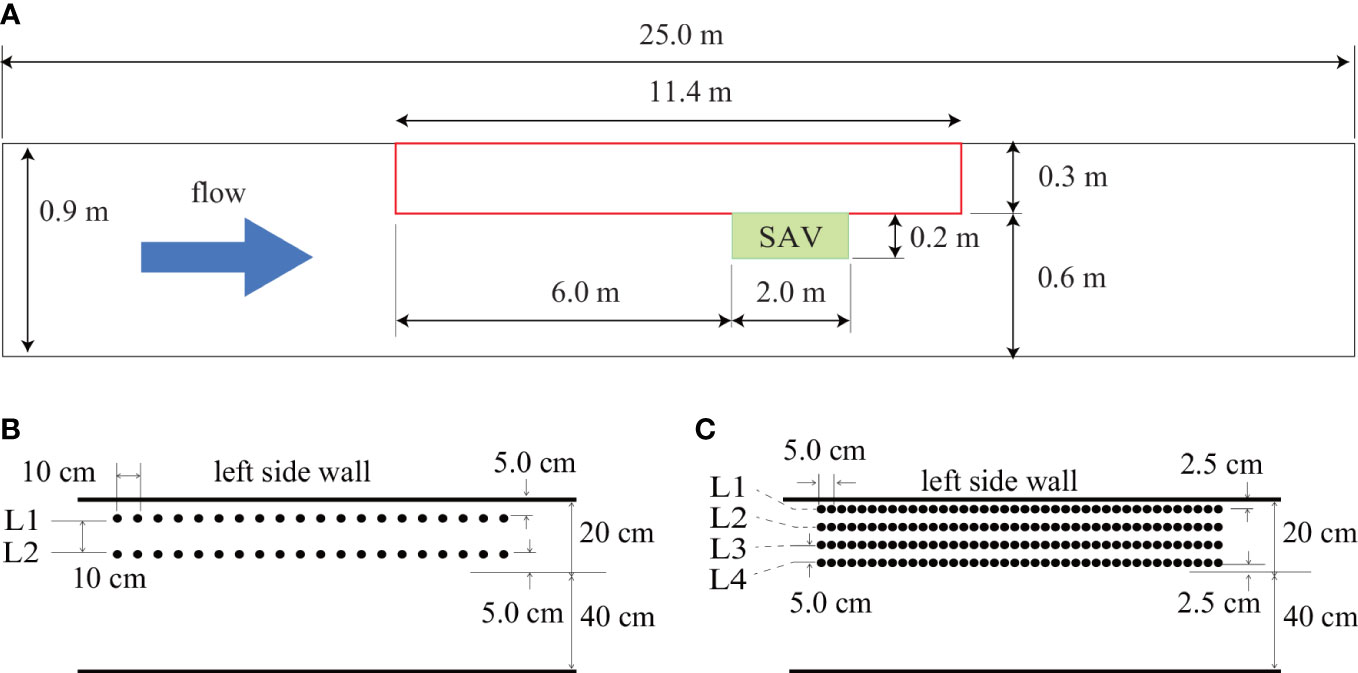
Figure 1 Open channel tank in the laboratory experiment. (A) The SAV replica was installed in the green-highlighted area. The SAV intervals were (B) 0.10 m and (C) 0.05 m.

TABLE 1

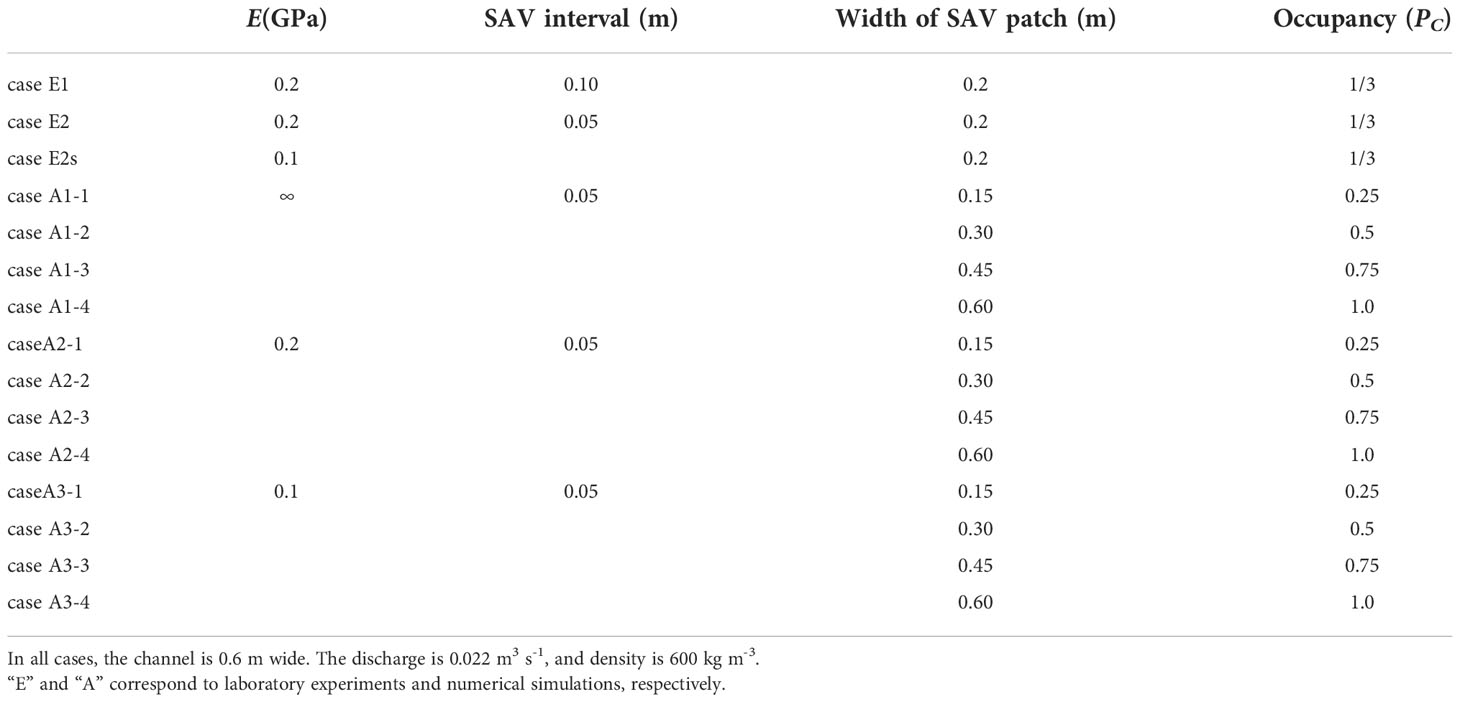
Table 1 Conditions for laboratory experiments and numerical simulations.

To mimic SAV patches, Luhar and Nepf (2011) attempted to use several kinds of materials in their laboratory experiments, such as high-density polyethylene and silicone foam, with densities of about 950 kg m^-3 and 600 kg m^-3, respectively. The elastic modulus of high-density polyethylene is about 1.0 GPa, and silicone foam has an elastic modulus of about 0.5 GPa. Nakayama et al. (2020b) demonstrated that the density and the elastic modulus of Zostera marina were 970 kg m^-3 to 995 kg m^-3 and about 1.0 GPa. Thus, superficial comparisons suggest that high-density polyethylene is similar to Zostera marina. However, we have a scale problem because eelgrass leaves grow to more than 1.0 m in length, 0.01 m in width, and 0.001 m thickness; it is not easy to conduct laboratory experiments using a tank with a water depth of more than 1.0 m. We attempted to use the ratio of the deflected vegetation height (DVH) to the leaf length as one of the similarity rules in order to decide on a material to replicate SAV. DVH is the height of a deflected SAV interacting with currents. In previous studies, interactions between SAV and flow have been evaluated based on the extent of the flow-induced reconfiguration of aquatic vegetation using the Cauchy number, Ca, and buoyancy parameter, B. Ca indicates the relative magnitude of the drag force and elasticity, and B indicates the relative magnitude of the buoyancy and elasticity. DVH is a function of the Cauchy number, Ca, and the buoyancy parameter, B (Luhar and Nepf, 2011).

\begin{array}{l} C a = \frac{1}{2} \frac{ρ C_{D} b U_{w}^{2} l^{3}}{E I} & (1) \end{array}

\begin{array}{l} B = \frac{(ρ - ρ_{v}) g b d l^{3}}{E I} & (2) \end{array}

\begin{array}{l} \frac{DVH}{l} = 1 - \frac{1 - 0.9 C a^{- 1 / 3}}{1 + C a^{- 3 / 2} (8 + B^{3 / 2})} & (3) \end{array}

Here, ρ is the water density (kg m^-3), ρ_v is the vegetation density (kg m^-3), b is the vegetation width (m), d is the vegetation thickness (m), l is the vegetation height without current (m), U_w is the horizontal velocity (m s^-1), g is the gravitational acceleration (m s^-2), C_D is the drag coefficient of SAV, and EI is the flexural rigidity (N m²).

Therefore, we may suggest modeling Ca and B in laboratory experiments similar to those in the field. It is possible to use a similar velocity in the laboratory experiment, but, as mentioned above, the leaf length and width of the leaf length and width of the replica leaf are less than those of an actual SAV leaf in nature. Thus, a less-elastic modulus and a denser replica are needed to give similar Ca and B. Thus silicone foam, rather than high-density polyethylene, is recommended in a tank with a water depth of 0.3 m. Note that the characteristics of the low-foam polyethylene used in this study are similar to those of silicone foam.

SAV model interaction with hydrodynamics

We used the SAV model developed by Nakayama et al. (2020b) to investigate the interactions between the flows and the flexible motion of SAV (Figure 2). Dividing each leaf into segments and nodes enables us to properly include the drag, friction, buoyancy, lift, and elastic forces. Also, the feedback forces from SAV to the flows are included, further contributing to the high fidelity of this realistic model. The computational domain was set at 250 m to remove the reflection effect of waves from the downstream end to the SAV meadow. This meadow was placed 30 m further from the upstream end to provide a steady uniform current to the SAV patch. The open channel width was 0.6 m. The finest grid size, 0.05 m, was used around the SAV meadow, and the grid size changed from 0.05 m to 0.1 m, 0.2 m, 0.25 m, 0.5 m, and 1 m as the distance from the SAV meadow increased. The vertical grid size was 2.5 cm, and the uniform inflow discharge was given at the upstream end, 0.022 m³ s^-1.

FIGURE 2

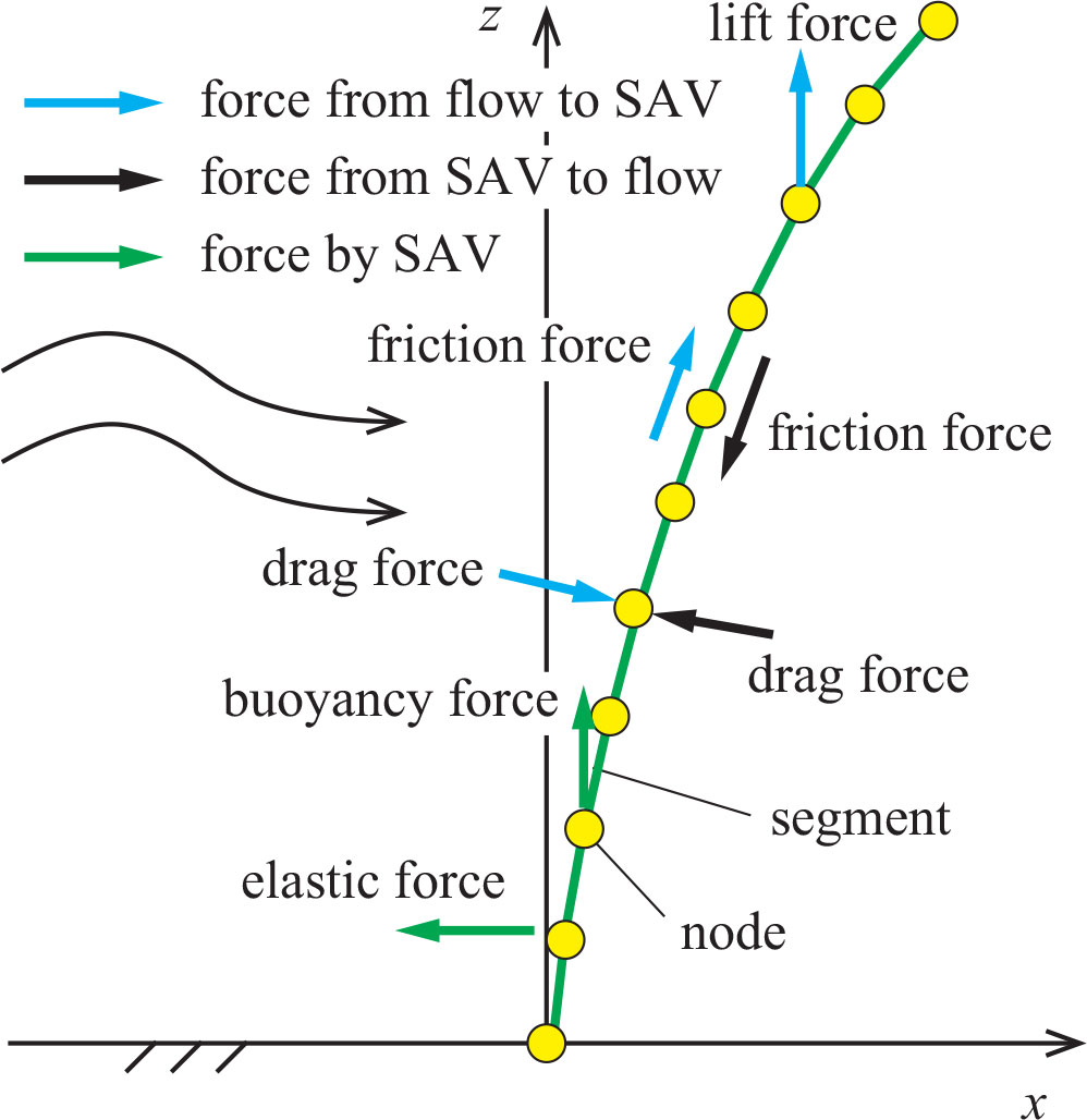
Figure 2 SAV model using segments and nodes. Blue arrows indicate the forces from the flow to the SAV. Black arrows indicate the reaction forces from the SAV to the flow. Green arrows indicate the forces due to buoyancy and elasticity.

\begin{array}{l} ρ_{a} V_{s} \frac{\partial u_{a}}{\partial t} = ρ_{w} \frac{| u - u_{a} | (u - u_{a})}{2} (C_{D} A_{x} + f_{c} A_{z}) - {(E I)}_{s} L_{s} \frac{\partial^{4} ξ_{x}}{\partial z^{4}} & (4) \end{array}

\begin{array}{l} ρ_{a} V_{s} \frac{\partial v_{a}}{\partial t} = ρ_{w} \frac{| u - u_{a} | (v - v_{a})}{2} (C_{D} A_{y} + f_{c} A_{z}) - {(E I)}_{s} L_{s} \frac{\partial^{4} ξ_{y}}{\partial z^{4}} & (5) \end{array}

\begin{array}{l} ρ_{a} V_{s} \frac{\partial w_{a}}{\partial t} = ρ_{w} \frac{| u - u_{a} | (w - w_{a})}{2} (C_{D} A_{z} + f_{c} \sqrt{A_{x}^{2} + A_{y}^{2}}) + ρ_{w} \frac{C_{L}}{2} {| u - u_{a} |}^{2} A_{x} + (ρ_{w} - ρ_{a}) g V_{s} & (6) \end{array}

In the equations above, ρ_a is the density of SAV (kg m^-3), V_s is the volume of a segment (m^-3), u is the vector of current velocity (m s^-1), u_a is the vector of SAV nodes (m s^-1), u is the horizontal current velocity (m s^-1), u_a is the horizontal velocity of SAV nodes (m s^-1), A_x is the vertical projected area in the x direction (m²), A_y is the vertical projected area in the y direction (m²), A_z is the horizontal projected area (m²), ξ_x is the displacement of nodes in the x direction (m), ξ_y is the displacement of nodes in the y direction (m), ρ_w is the water density (kg m^-3), C_D(= 1.3) is the drag coefficient of SAV, f_c(= 0.3) is the friction coefficient of SAV, C_L(=0.1) is the lift force coefficient of SAV, E is the elastic modulus (N m^-2), I is the second moment of inertia (m⁴), L_s is the length of a segment, v is the current velocity in the y direction (m s^-1), v_a is the velocity of SAV nodes in the y direction, w is the vertical current velocity (m s^-1), and w_a is the vertical velocity of SAV nodes (m s^-1).

Results

Velocities and deflected vegetation height

We found that DVH on L1 and DVH on L2 were not significantly different in case E1, where the SAV interval was 0.1 m in the laboratory experiments (Figure 3). In contrast, the deflection was significantly greater on L4 than on L1 in case E2, with an SAV interval of 0.05 m. Since SAV aggregated more in case E2 than in case E1, and the bulk drag force was larger in case E2, we conclude that the flow went around the front of the SAV patch in case E2 more than in case E1, resulting in a more significant deflection on L4 than on L1. PIV provided satisfactory horizontal velocities in case E1 (Figure 4). However, there were substantial fluctuations in case E2 because it was difficult to remove the silhouette of the SAV patches due to the high density of SAV, which also made it impossible to make the velocity measurements from 0.06 m to 0.10 m in the vertical axis.

FIGURE 3

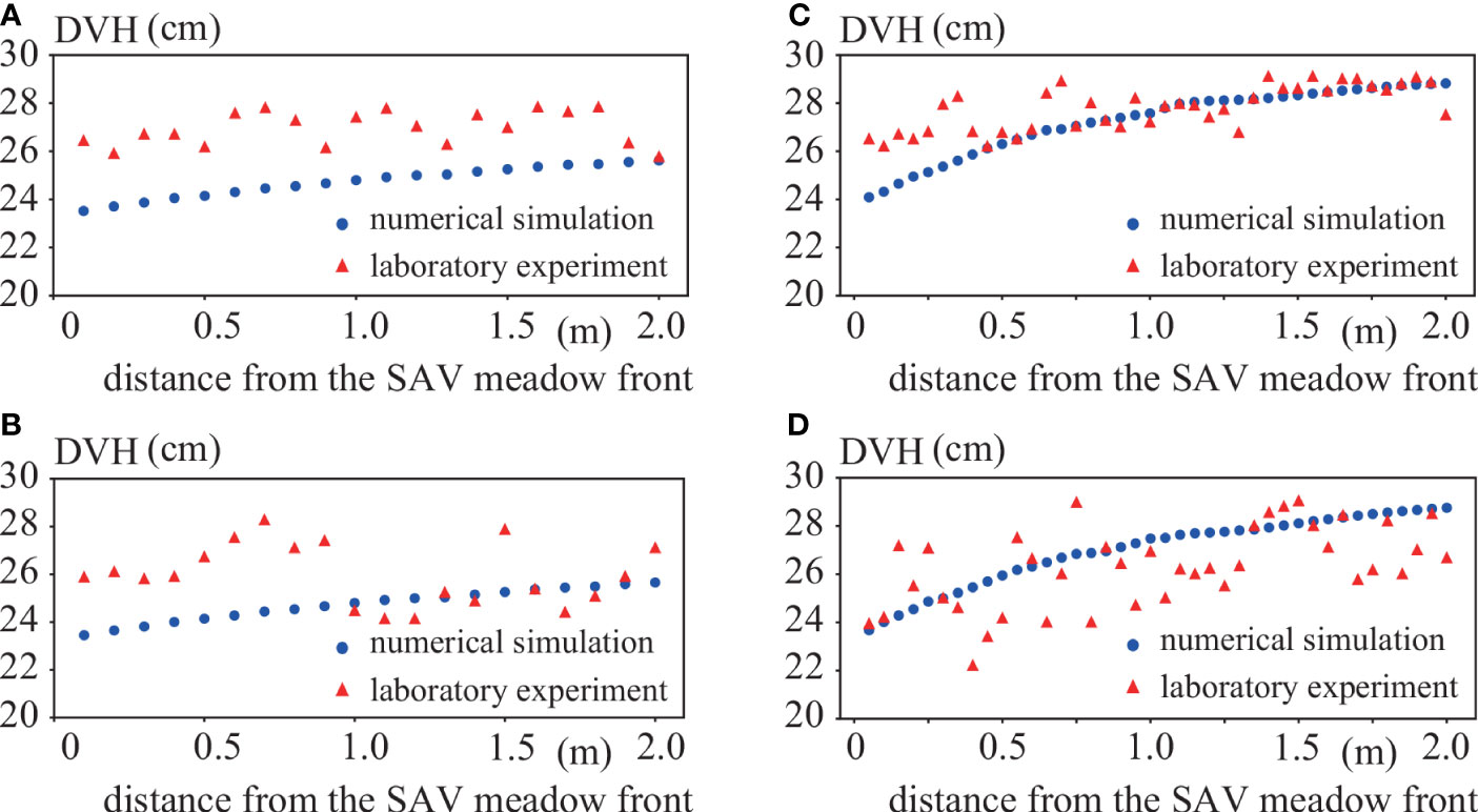
Figure 3 Comparisons of DVH between laboratory experiments and numerical simulations. Blue circles and red triangles indicate the laboratory experiment and the numerical simulation, respectively. (A) L1 in case E1, (B) L2 in case E1, (C) L1 in case E2, (D) L4 in case E2.

FIGURE 4

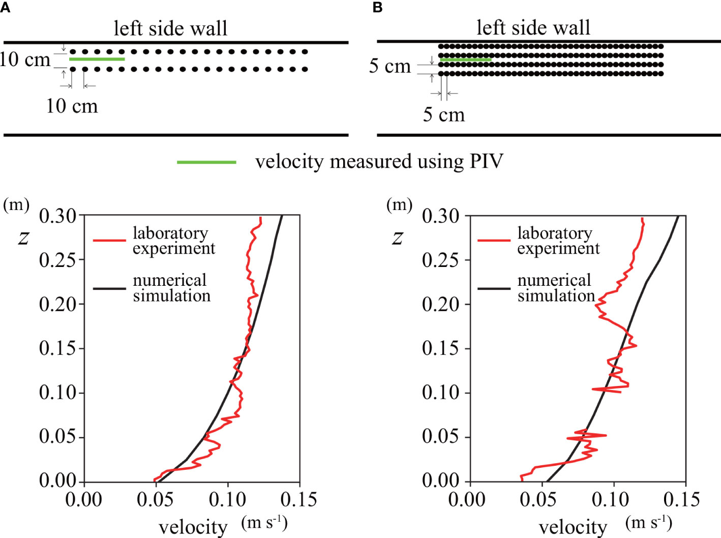
Figure 4 Comparison of the vertical profiles of horizontal velocities between laboratory experiments and numerical simulations. Red and black lines indicate the laboratory experiment and the numerical simulation, respectively. (A) Case E1, (B) Case E2.

Influence of SAV on flows in the laboratory experiments

The SAV model agreed well with the laboratory experiments in regard to the root mean squared percentage error (RMSPE) for the DVH (Table 2), which was calculated as

TABLE 2

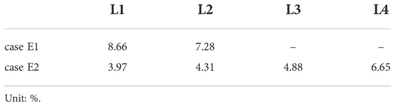
Table 2 Root mean squared percentage error (RMSPE) on DVH between laboratory experiments and numerical simulations.

\begin{array}{l} RMSPE = \sqrt{\frac{1}{N} \sum_{i = 1}^{N} {(\frac{y_{n, i} - y_{e, i}}{y_{e, i}})}^{2}} & (7) \end{array}

where N is the number of samples, y_n,i is the computed DVH, and y_e,i is the measured DVH.

A numerical simulation showed the same tendency, i.e., the DVH on L1 in case E1 was almost the same as that on L2 (Figures 3A, B). In contrast to case E1, in case E2 the DVH on L4 was slightly smaller than that on L1, though the DVH difference from the laboratory experiments was more significant than that in the SAV model (Figures 3C, D). The velocities obtained by the PIV agreed very well with the numerical simulation in case E1 (Figure 4A). Although there were large fluctuations in the PIV in case E2, the velocities mostly agreed between the laboratory experiment and the numerical simulations (Figure 4B).

To understand the effect of elasticity on the flows around an SAV patch, we conducted a numerical simulation in which the elastic modulus was half that in case E2; this new case is called case E2s (Table 1). The maximum velocity occurred at the front above the SAV meadow on L4 in case E2, which caused a more significant deflection on L4 than on L1 (Figure 5B). However, the maximum velocity occurred at the end above the SAV on L4 in case E2s (Figure 5D). In addition, the velocity reduction inside the SAV meadow was more remarkable in case E2s than in case E2.

FIGURE 5

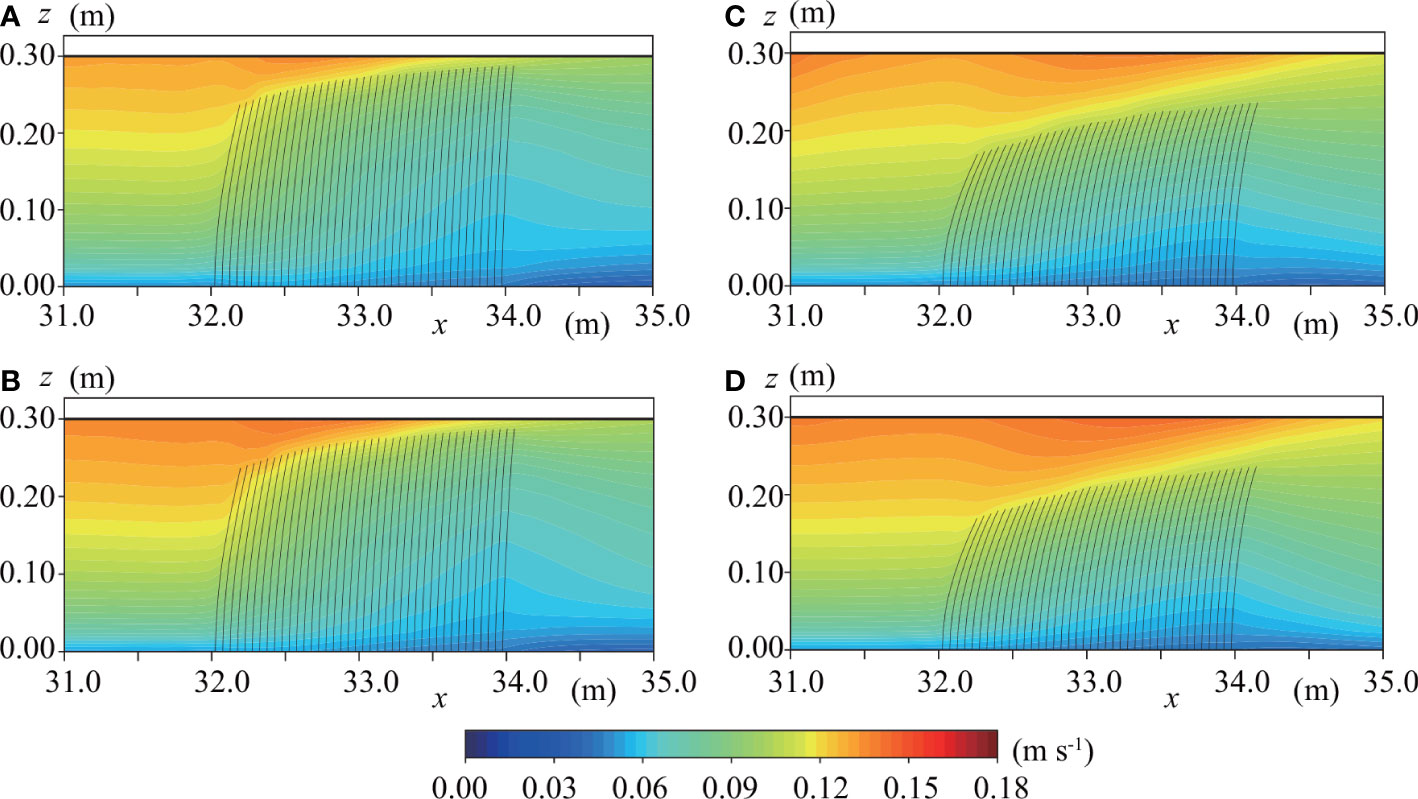
Figure 5 Horizontal velocity distributions at (A) L1 in case E2, (B) L4 in case E2, (C) L1 in case E2s, and (D) L4 in case E2s.

Influence of elasticity and the patch occupancy on flows

To investigate the effect of patch occupancy on water flows, we compared the horizontal velocity between occupancies of 25% and 100% for cases A1 to A3 (Figure 6). The horizontal velocity at the SAV patch center is smaller in the case with an occupancy of 25% than in the case with an occupancy of 100% because the currents go around the SAV patch. Moreover, the horizontal velocity inside an SAV patch is significantly lower at 25% compared to 100% occupancy. Additionally, it is apparent that the lower the elasticity, the greater the horizontal velocity above the SAV meadow. Since more water goes around the SAV patch at an occupancy of 25% than at an occupancy of 100%, the SAV bends more in the latter case.

FIGURE 6

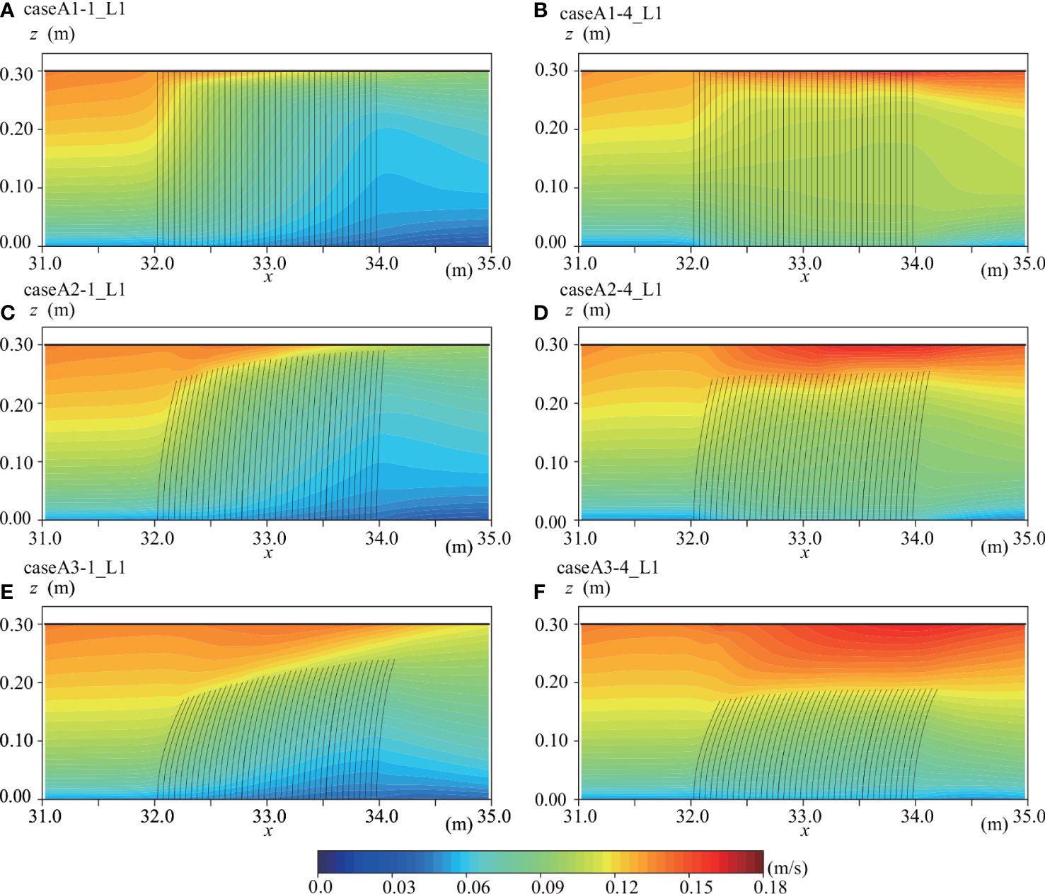
Figure 6 Horizontal velocity distributions at L1 in (A) case A1-1, (B) case A1-4, (C) case A2-1, (D) case A2-4, (E) case A3-1, and (F) case A3-4.

Since the results shown in Figure 6 indicated the significance of the water flows around an SAV patch, we next investigated the elasticity effect on the dominant currents at an occupancy of 50% (Figure 7). When there is no elasticity, the horizontal velocity is the largest at L5 of case A1-2, and the water flows most significantly around the SAV patch (Figures 7A, B). In case A3-2, the water flows above the SAV patch, resulting in the smallest horizontal velocity at L5 among cases with an occupancy of 50%.

FIGURE 7

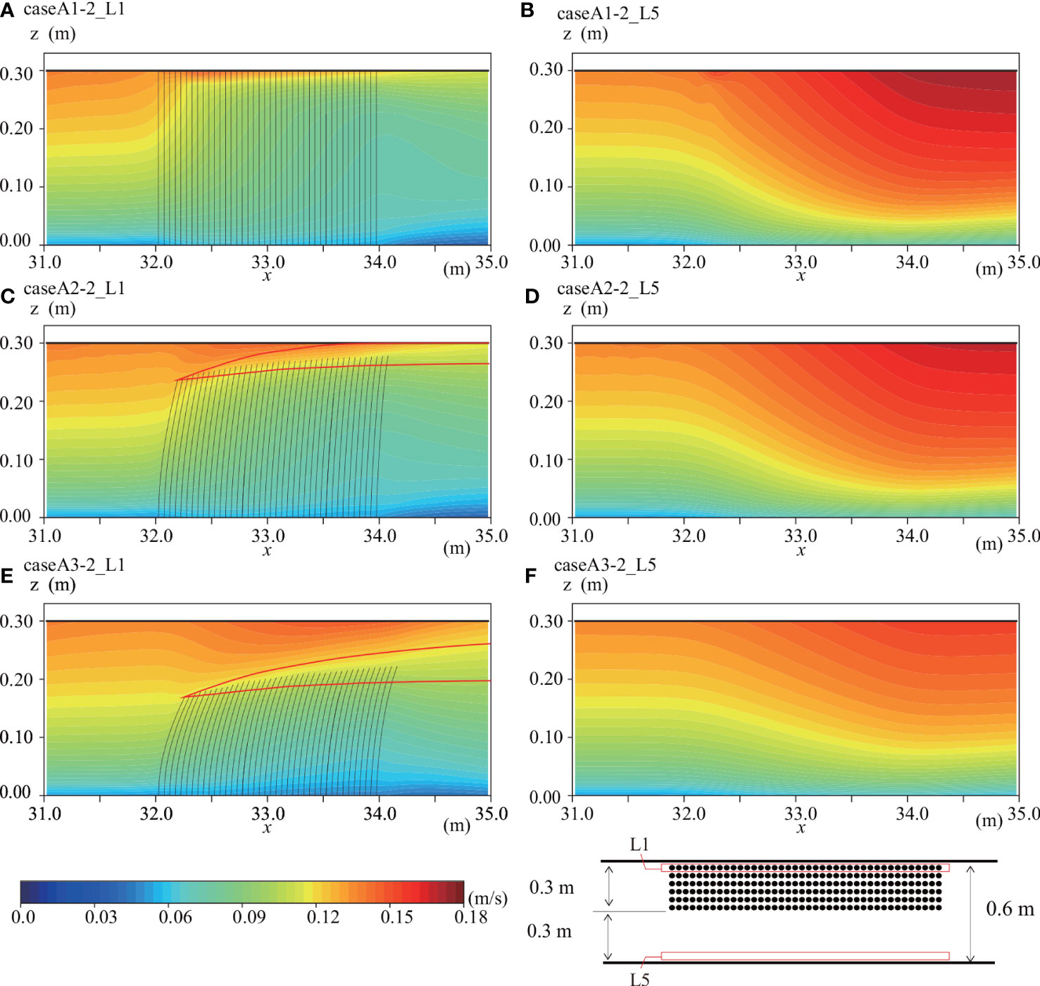
Figure 7 Horizontal velocity distributions at (A) L1 in case A1-2, (B) L5 in case A1-2, (C) L1 in case A2-2, (D) L5 in case A2-2, (E) L1 in case A3-2, and (F) L5 in case A3-2.

Discussion

Luhar and Nepf (2011) successfully proposed an equation to predict the DVH. However, they found that their equation overestimated the drag force when Ca >> 1.0. In this study, therefore, to investigate the validity and robustness in the SAV model reconfigured using the equation of Luhar and Nepf, we compared the DVH for a single leaf blade (Table 3). In our study, Ca was 15.01 and B was 6.35 for one blade with a length of 0.3 m. Therefore, the drag force was overestimated in the theoretical solution, as we expected. Still, the SAV model predicted the DVH almost perfectly, suggesting the effectiveness of this model for analyzing various types of submerged aquatic vegetation (Figure 8).

TABLE 3

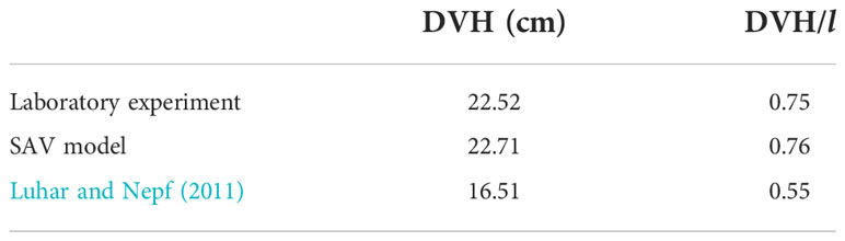
Table 3 Comparisons of DVH for one blade.

FIGURE 8

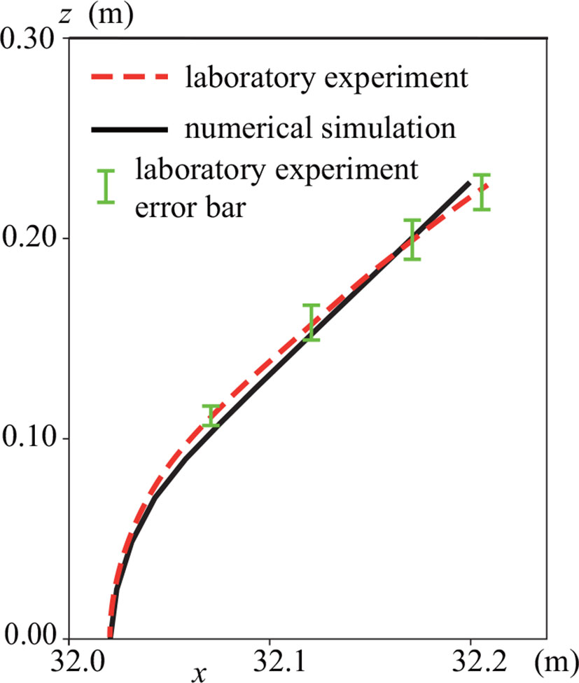
Figure 8 Blade shapes of laboratory experiments and numerical simulations. Black solid and red broken lines are the model predictions and measured postures. Vertical green bars indicate the error bar, which was calculated by averaging the results of the three experiments.

Duarte et al. (2013) demonstrated that the velocity inside the SAV meadow decreased due to the deflection enhancing the current above the meadow, resulting in the accumulation of particulate organic carbon and nutrients. The SAV model also showed a similar reduction of currents inside the meadow with a high-speed current above it (Figure 5). This may suggest that the current tends to go around an SAV patch when the level of SAV bending is low, but over the patch when the level of SAV bending is high (Figures 7, 9).

FIGURE 9

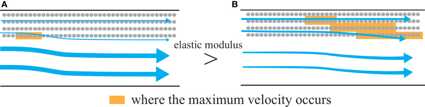
Figure 9 Flow modification due to an SAV patch. Arrows indicate the mean fluxes on a horizontal plane. The elasticity is larger in case E2 than in case E2s, resulting in the larger DVH in case E2 than in case E2s. (A) Case E2, (B) case E2s.

Adams et al. (2016) demonstrated the importance of the blade bending angle on water movement and turbidity inside a seagrass meadow. The more the blade bends, the more significantly the sediment is accumulated. It is apparent that the smaller elasticity, the lower the DVH when occupancy is 100% (Pc = 1.0 in Figure 10). Intriguingly, the DVH increases linearly with the decrease in occupancy (Pc). Furthermore, the reduction rate of DVH by Pc is almost the same between cases A2 and A3. Therefore, the DVH was likely predicted by Pc in our experiments using DVH with an occupancy of 100%, even though we did not conduct numerical simulations with other occupancy ratios.

FIGURE 10

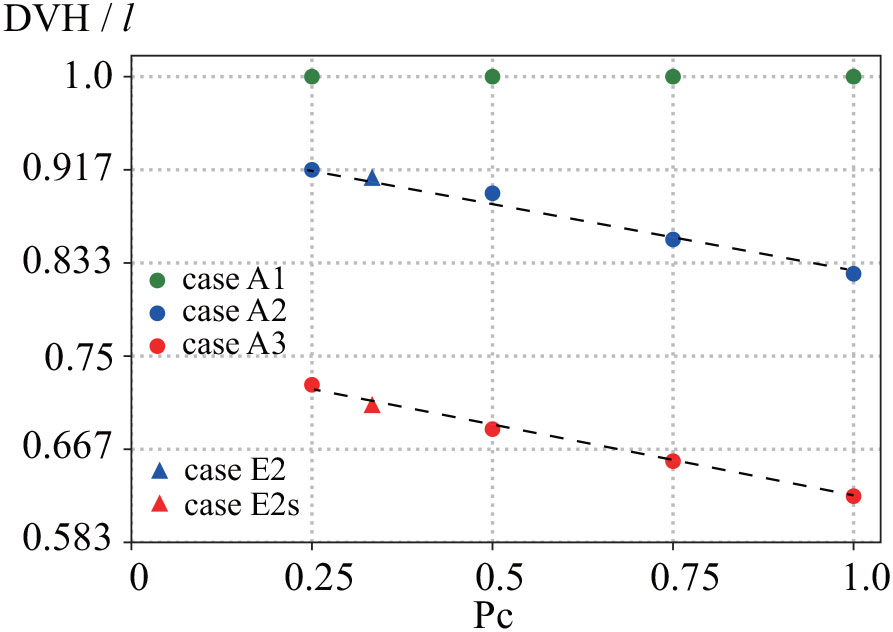
Figure 10 DVH obtained from numerical simulations for cases E2 and E2s, and cases A1 to A3. Broken lines indicate the approximate straight lines obtained using the least-squares method.

To investigate the decrease in velocity inside the SAV meadow due to the blade bending (Duarte et al., 2013) from the perspective of flux, we computed the normalized discharge inside an SAV patch. The normalization was done using the discharge with an occupancy of 100% and no elasticity blade (Figure 11). Similar to the results for DVH, we found that the smaller the elasticity, the less the normalized flux inside an SAV patch when the occupancy was 100% (Pc = 1.0 in Figure 11). Importantly, the normalized flux inside an SAV patch for each elasticity was revealed to be a linear function of Pc (blue and red solid lines in Figure 11). Therefore, the normalized flux inside an SAV patch can be predicted by Pc using the normalized flux with an occupancy of 100% for each elasticity. Note that the normalized flux inside an SAV patch cannot be modelled using a linear function when there is no blade bending. Conditions that do not include blade bending may have different characteristics compared to those which incorporate blade bending, suggesting the necessity of a model that includes blade bending in order to analyze the water flows and mass transport around the SAV meadow.

FIGURE 11

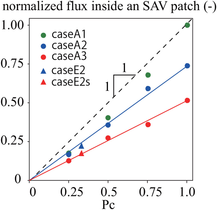
Figure 11 Normalized flux inside an SAV patch from numerical simulations for cases E2 and E2s, and cases A1 to A3. Blue and red solid lines indicate the approximate straight lines obtained using the least-squares method.

Ghisalberti and Nepf (2006) demonstrated that a typical boundary layer is present along the top of the seagrass meadow. In our numerical simulations, we also confirmed the occurrence of a mixing boundary layer along the top of SAVs (the regions enclosed by red lines in Figures 7C, E). Here, the important point is that the boundary layer cannot reach the water surface when a blade bending angle is large (Figure 7E). Therefore, we hypothesize that the carbon flux between the atmosphere and the water surface proceeds as shown in Figure 12. The pCO2 inside an SAV patch is lower than that in the atmosphere due to the photosynthesis activity during the daytime (Figure 12). However, the blade bending angle is too large to enable the boundary layer to reach the water surface, suggesting that the absorption of pCO2 from the atmosphere would be lower (Figure 12). Therefore, it is necessary to investigate the SAV motion under the currents and waves to clarify the pCO2 flux between the atmosphere and the water surface.

FIGURE 12

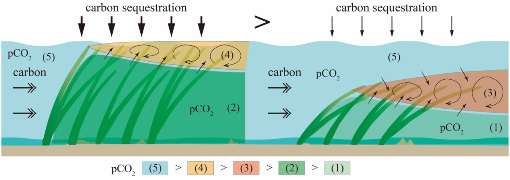
Figure 12 Carbon dioxide flux difference due to the formation of a mixing boundary layer at the top of the SAV meadow and DVH.

Conclusion

The SAV numerical model was successfully applied to analyze flows around a patch-like SAV meadow, and the results were in good agreement with those of the laboratory experiments. Numerical simulations revealed that, when the SAV bended considerably, larger velocities occurred above the SAV meadow, with the lowest velocity being adjacent to the SAV bottom. When the SAV did not bend significantly, the velocities went around the SAV meadow more substantially than they did in the low-elastic modulus case. The extent to which the patch occupies the channel width was revealed to be the most substantial factor in controlling hydrological conditions and mass transport due to SAV, and deflection was found to be another important factor. Planning and implementing global warming countermeasures are acute goals for climate change mitigation, and efficient planting and management of SAV are urgently needed. Therefore, our study outcome is expected to make an important contribution to the improvement of SAV models that can eventually be applied to quantify the enhancement of blue carbon as a negative emission strategy.

Data availability statement

The raw data supporting the conclusions of this article will be made available by the authors, without undue reservation.

Author contributions

KM: Formal analysis, Investigation, Writing – Original Draft. KN: Funding acquisition, Conceptualization, Methodology, Investigation, Formal analysis, Investigation, Writing – Original Draft. HM: Methodology, Investigation, Formal analysis, Writing – Review & Editing. All authors contributed to the article and approved the submitted version.

Funding

This work was supported by the Japan Society for the Promotion of Science under grant nos. 22H01601, 22H05726, and 18KK0119. The authors declare that they have no conflicts of interest.

Conflict of interest

The authors declare that the research was conducted in the absence of any commercial or financial relationships that could be construed as a potential conflict of interest.

Publisher’s note

All claims expressed in this article are solely those of the authors and do not necessarily represent those of their affiliated organizations, or those of the publisher, the editors and the reviewers. Any product that may be evaluated in this article, or claim that may be made by its manufacturer, is not guaranteed or endorsed by the publisher.

References

Abdelrhman M. A. (2007). Modeling coupling between eelgrass zostera marina and water flow. Mar. Ecol. Prog. Ser. 338, 81–96. doi: 10.3354/meps338081

ORIGINAL RESEARCH article

Influence of patch size on hydrodynamic flow in submerged aquatic vegetation

Introduction

Materials and methods

Laboratory experiments

SAV model interaction with hydrodynamics

Results

Velocities and deflected vegetation height

Influence of SAV on flows in the laboratory experiments

Influence of elasticity and the patch occupancy on flows

Discussion

Conclusion

Data availability statement

Author contributions

Funding

Conflict of interest

Publisher’s note

References

This article is part of the Research Topic

People also looked at