Evaluation of Regional Surface Energy Budget Over Ocean Derived From Satellites

Introduction

Estimating the surface energy budget is one of the key components of understanding energy flow within the Earth system. Surface energy fluxes determine the energy input to the ocean and energy transfer through the ocean-atmosphere boundary. In addition, surface fluxes often drive processes occurring near the surface. For example, energy fluxes at the surface affect cloud processes occurring in the boundary layer (e.g., Betts, 1985; Betts and Ridgway, 1988; Albrecht et al., 1990; Bretherton and Wyant, 1997; Wood, 2012). In addition, surface radiative fluxes play a key role in determining sea ice melts (Hudson et al., 2013). Both low-level clouds (Soden et al., 2008; Loeb et al., 2018) and sea ice play a critical role determining climate feedback and Earth’s energy budget (Hartmann and Ceppi, 2014).

Components of the surface energy flux are radiative flux (irradiance), turbulent flux, and flux associated with mass transfer. Surface irradiance is composed of shortwave and longwave irradiances. Downward surface shortwave irradiance is the solar irradiance transmitted through the atmosphere. Part of the irradiance that reaches the surface is reflected by the surface, which can be reflected back to the surface by the atmosphere, and the rest is absorbed by the surface. Broadband ocean surface albedo is about 0.05 (e.g., Kato et al., 2002) but the albedo depends on solar zenith angle and surface wind speed (Cox and Munk, 1955) and chlorophyll concentration (Jin et al., 2004). Downward surface longwave irradiance is the emitted irradiance by the atmosphere. Similar to the shortwave irradiance, a part of the downward longwave irradiance is reflected and the rest is absorbed by the surface. The surface also emits longwave irradiance, with a magnitude depending on the temperature and emissivity, with the latter being a function of wind speed over ocean (Sidran, 1981; Masuda et al., 1988).

Turbulent heat fluxes consist of sensible and latent heat fluxes. These are enthalpy fluxes and depend on near surface and surface properties (e.g., Cronin et al., 2019). In addition to these enthalpy fluxes, the enthalpy is transferred through the atmosphere-ocean boundary when water is transported by precipitation and evaporation (Mayer et al., 2017; Trenberth and Fasullo, 2018; Kato et al., 2021).

From a regional ocean energy budget perspective, surface fluxes are needed to separate the energy input from that by horizontal energy transport by ocean, provided that the regional ocean temperature tendency is known (Trenberth and Solomon, 1994). Despite the importance of surface energy fluxes, there is a large uncertainty associated with surface fluxes derived from satellite observations. The uncertainty in the regional monthly mean net surface irradiance over ocean estimated by Kato et al. (2020) is 13 Wm^–2. Similarly, a typical error in a long-term mean net energy flux over ocean is 10 Wm^–2 (Cronin et al., 2019). In addition, temperatures of raindrops and water vapor are needed to estimate the enthalpy transfer associated with water mass transfer (Mayer et al., 2017; Kato et al., 2021). As a consequence, when satellite derived surface flux data products are integrated to assess the surface energy balance, the residual of annual global surface energy balance is about 10–15 Wm^–2 (Kato et al., 2011; Stephens et al., 2012; Loeb et al., 2014; L’Ecuyer et al., 2015; Wild et al., 2015). Therefore, annual net surface energy fluxes averaged over global ocean is one order of magnitude larger (Meyssignac et al., 2019) than the mean ocean heating rate of 0.8 Wm^–2 (Johnson et al., 2016; Loeb et al., 2018; von Schuckmann et al., 2020).

Computed surface fluxes have been evaluated using observations. However, the spatial and temporal coverage of surface observations are limited. Comparisons of similar data products are useful to identify outliers and unphysical assumptions. Even though the regional energy budget bias in satellite-based data products is significant, the bias can be explained by the sum of uncertainties of all components (L’Ecuyer et al., 2015). A less explored approach for evaluating energy budget flux products is to use horizontal energy transport by the atmosphere and to compare the resulting net surface energy flux with the sum of surface energy flux components. In this study, we integrate surface energy data products and demonstrate the use of energy divergence in the atmosphere in evaluating surface energy flux data products. In addition, we examine regional water mass balance to understand whether the regional water mass balance residual can explain the energy balance residual. Furthermore, we analyze the seasonal variability of surface energy fluxes to test whether the variability can be used in the evaluation. If the physical processes are robust, the seasonal variability might be used to evaluate the quality of energy data products.

Section “Regional Water Mass and Atmosphere Energy Budget Equations” introduces regional energy and water mass budget equations that are used in this study. Data products used in this study are described in section “Data Products.” Regional net surface energy flux and mass balance, as well as seasonal variability of surface energy fluxes are discussed in section “Results.”

Regional Water Mass and Atmosphere Energy Budget Equations

One form of energy balance equations of an atmospheric column is the balance between energy tendency in the column and fluxes at boundaries, i.e., top-of-atmosphere (TOA), lateral boundaries, and at surface boundary (Trenberth, 1997). The energy flux at the top boundary is the net TOA irradiance R_TOA. R_TOA is the sum of absorbed shortwave irradiance, which is the insolation minus reflected shortwave irradiance and emitted longwave irradiance multiplied by −1 (because the net is defined downward positive in this study). Fluxes at the surface include net surface irradiance R_sfc, sensible heat flux F_SH and latent heat flux F_LH, and enthalpy flux associated with precipitation F_fallout and evaporation F_v. The atmosphere can transport enthalpy, potential energy and kinetic energy through lateral boundaries. The energy budget equation of an atmospheric column is then expressed as (Mayer et al., 2017; Trenberth and Fasullo, 2018; Kato et al., 2021),

where U_a is the dry air horizontal velocity, c_p is the specific heat capacity, T is the temperature, Φ is the geopotential, Φ_s is the surface geopotential, k is the kinetic energy, p is the pressure, p_sfc is the surface pressure, t is time, and g is the gravitation acceleration at sea level. All energy terms include contributions from dry air, water vapor and hydrometeors and they are added weighted by their respective mixing ratios r,

where c_{p_a}is the specific heat capacity of dry air at constant pressure, c_{p_v} is the specific heat capacity of water vapor at constant pressure, and c is the specific heat capacity of hydrometeors. Subscripts v, l, i, r, s are, respectively, water vapor, liquid and ice cloud particles, rain, and snow. The latent heat l is the sum of the enthalpy change when water vapor is condensed or hydrometeors are evaporated,

l_v is the enthalpy of vaporization, l_f is enthalpy of fusion, r is the mixing ratio. The latent heat is determined by the enthalpy release when water vapor is condensed or snow and ice crystals are melted. Therefore, l_l in this case is the specific heat capacity multiplied by the temperature difference between cloud particles or raindrops and the reference temperature. The F_h term on the right side of Eq. 1 represents the divergence of moist static and kinetic energy associated with hydrometeors moving at different velocities from the dry air velocity (Kato et al., 2021),

Because F_h is not provided by data products used in this study, we assume that velocities of all hydrometeors are equal to the dry air velocity (i.e., F_h=0). The enthalpy fluxes associated with water mass transfer F_m are the sum of,

and

where c_w is the specific heat capacity of either ice or liquid water, T_w is 2 m wet bulb temperature, T_skin is the ocean skin temperature, T₀ is 0°C (Mayer et al., 2017; Trenberth and Fasullo, 2018), $\stackrel{.}{P}$ is the precipitation rate and $\stackrel{.}{E}$ is the evaporation rate.

The energy balance Eq. 1 suggests two possible ways of computing net surface energy flux. One way is to use all the surface flux components,

where F_net,c is positive downward (hereinafter the component approach). The second method for deriving the net surface flux suggested by Eq. 1 is to use TOA net irradiance, atmospheric divergence, and tendency terms (hereinafter the transport approach),

This approach is used by, for example, Trenberth (1997); Trenberth et al. (2001), Trenberth and Stepaniak (2004); Liu et al. (2015), and Mayer et al. (2017); Trenberth and Fasullo (2018), and Liu et al. (2020). Similar to the energy balance Eq. 1, the water mass balance equation for an atmospheric column is (Trenberth, 1991),

where

and the precipitation rate $\stackrel{.}{P}={\stackrel{.}{P}}_r+{\stackrel{.}{P}}_s$ is the sum of rain and snow rates. Eq. 11 states that the tendency and convergence of water mass is balanced with the difference of precipitation and evaporation rates at the surface. Because of the assumption of hydrometeors traveling with the dry air velocity, F_r = 0. The energy balance Eq. 1 and water mass balance Eq. 11 are related through the diabatic heating term in the total energy equation of the atmospheric column (e.g., Kato et al., 2021).

Data Products

The TOA and surface irradiance data product used in this study is the Edition 4.1 Clouds and the Earth’s Radiant Energy System (CERES) Energy Balance and Filled (EBAF). Global net TOA irradiances averaged over 10 years from July 2005 to June 2015 is adjusted to 0.71 Wm^–2 based on ocean heating rates, ice warming and melts, and atmospheric and lithospheric warming (Johnson et al., 2016; Loeb et al., 2018). A detailed description of the method to produce TOA and surface irradiances included in the product and their uncertainty are given, respectively, in Loeb et al. (2018) and Kato et al. (2018). Horizontal transport of moist static energy and water vapor, as well as surface turbulent fluxes are derived from the ERA-Interim reanalysis data product (Dee et al., 2011). Although mass is not conserved in the original data product (Mayer et al., 2017; Trenberth and Fasullo, 2018; Liu et al., 2020), it is conserved in the ERA-Interim data product used in this study. Mass correction procedures and the method to compute horizontal transport are discussed in Trenberth and Fasullo (2018). Two other sets of surface turbulence fluxes used in this study are Version 3 SeaFlux data product (Roberts et al., 2020) and the Version 3 of the Objectively Analyzed Air-sea Fluxes (OAFlux) (Yu et al., 2008). Precipitation rate data product used in this study is Version 2.3 Global Precipitation Climatology Project (GPCP) data product (Adler et al., 2012). EBAF irradiances, SeaFlux turbulent fluxes, and GPCP precipitation rates are derived using primarily satellite observations. The time period used in this study is from January 2001 to December 2016.

Results

In this section, we investigate the consistency of regional surface energy budget derived by two different approaches (Eqs. 9, 10). Seasonal variabilities of surface net energy fluxes averaged over 45°N to 45°S ocean are compared to check the consistency of the temporal variability.

Regional Surface Energy Budget and Water Mass Balance

Figure 1 shows four surface energy flux components that appear on the right side of Eq. 1. The net irradiance R_sfc is primarily a function of latitude. A positive net irradiance over the tropical ocean is largely compensated by latent heat flux F_LH. Sensible heat flux F_SH is much smaller than F_LH. In addition, the meridional gradient of F_SH is much smaller than the meridional gradient of R_sfc and F_LH. The spatial pattern of the enthalpy flux associated with water mass transfer F_m resembles the spatial pattern of precipitation rate. When these components are averaged over the global open water, R_sfc, F_LH, F_SH, and F_m are, respectively, 126, −97, −12, and −1 Wm^–2. The sum of these four components is 16 Wm^–2, which is one order of magnitude larger than the annual global mean ocean heating rates. Note that the annual global mean ocean heating rate given in Johnson et al. (2016) of 0.68 Wm^–2 is averaged over the entire global area. Therefore, the ocean heating rate averaged over the global ocean is 0.93 Wm^–2, which is estimated as the product of 0.68 Wm^–2 and the ratio of the global area to the ocean area of 1.37 (=0.510 / 0.372). We ignore enthalpy transported to the global ocean by river runoff, which is about 10% of water evaporated from the ocean (Rodell et al., 2015).

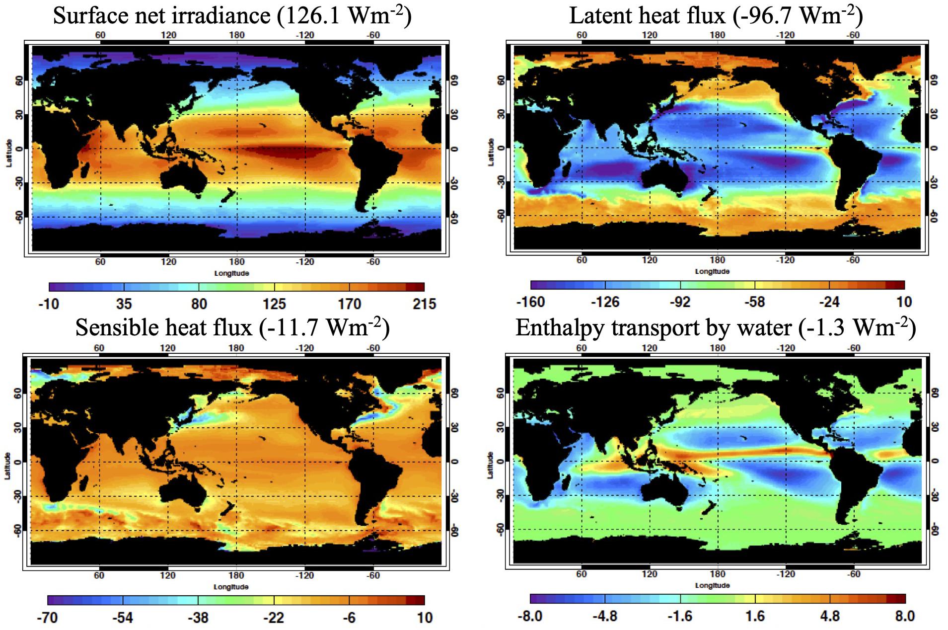
Figure 1. (Top left) Surface net irradiance derived from Edition 4.1 Energy Balance and Filled (EBAF) product, (top right) latent heat flux derived from Version 3 SeaFlux product, (bottom left) SeaFlux sensible heat flux, and (bottom right) enthalpy flux associated with water mass transfer derived from Version 2.3 Global Precipitation Climatology Project (GPCP) and SeaFlux. All maps are climatological mean values from January 2001 to December 2016. Net irradiance and fluxes are defined positive downward. Units is Wm^{– 2} for all plots. Mean values averaged over the global ocean are shown with titles.

The regional energy budget computed by Eq. 9 F_net,c, expressed as the sum of R_sfc, F_LH, F_SH, and F_m, is shown in the left panel of Figure 2. A positive value indicates that net energy is transferred to the ocean. The right panel of Figure 2 also shows the regional energy budget computed by Eq. 10 F_net,t. The net surface flux F_net,t averaged over the global open water is 2.1 Wm^–2, whereas its F_net,c counterpart is 16.3 Wm^–2. Mayer et al. (2021) who computed net surface energy flux over ocean with ECMWF ERA5 (Hersbach et al., 2018) by the transport approach report F_net,t of 1.6 Wm^–2. Josey et al. (2013) who computed net surface energy flux over ocean with OAFlux turbulent fluxes (Yu and Weller, 2007) and International Satellite Cloud Climatology Project (ISCCP) irradiances (Zhang et al., 2004) by the component approach report F_net,c of 29 Wm^–2. The difference between F_net,c and F_net,t is the atmospheric energy balance residual ε_E,

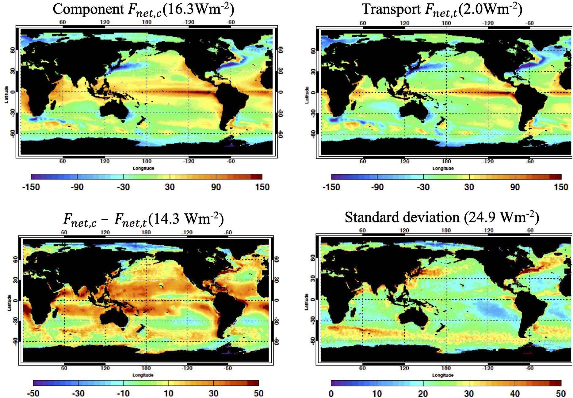
Figure 2. (Top left) Regional net surface energy flux computed with net irradiance, sensible and latent heat fluxes, and enthalpy flux associated with water mass transfer (component approach F_net,c) (Top right) Regional net surface energy flux computed with top-of-atmosphere (TOA) net irradiance, moist static divergence, and moist static energy tendency (transport approach F_net,_t). (Bottom left) Difference of regional net surface energy fluxes, F_net,c – F_net,t. (Bottom right) standard deviation of reginal monthly F_net,_c – F_net,_t computed over 192 months. All maps are climatological mean values from January 2001 to December 2016. Net irradiance and fluxes are defined positive downward. Units is Wm^{– 2} for all plots. Mean values averaged over global ocean are shown with titles.

The difference between F_net,c and F_net,t exists over tropics (bottom left plot of Figure 2). Spatial distribution of F_net,t is not necessarily correct, but a casual comparison for F_net,c and F_net,t showing large ε_E over the tropics leads us to conclude that the tropical region is largely responsible for the larger energy budget residual from the component approach. The standard deviation over the tropics (bottom right plot of Figure 2) is nearly equal to ε_E over the tropics while it is larger than ε_E over mid-latitude. This indicates that seasonal variability of ε_E is small over the tropics, but larger seasonal variability exists over mid-latitude. Note that the spatial pattern of ε_E shown in the bottom left plot of Figure 2 differs from the spatial pattern of Figure 3 of Kato et al. (2016) because different energy balance equations of an atmospheric column, hence different energy flux data products, are used.

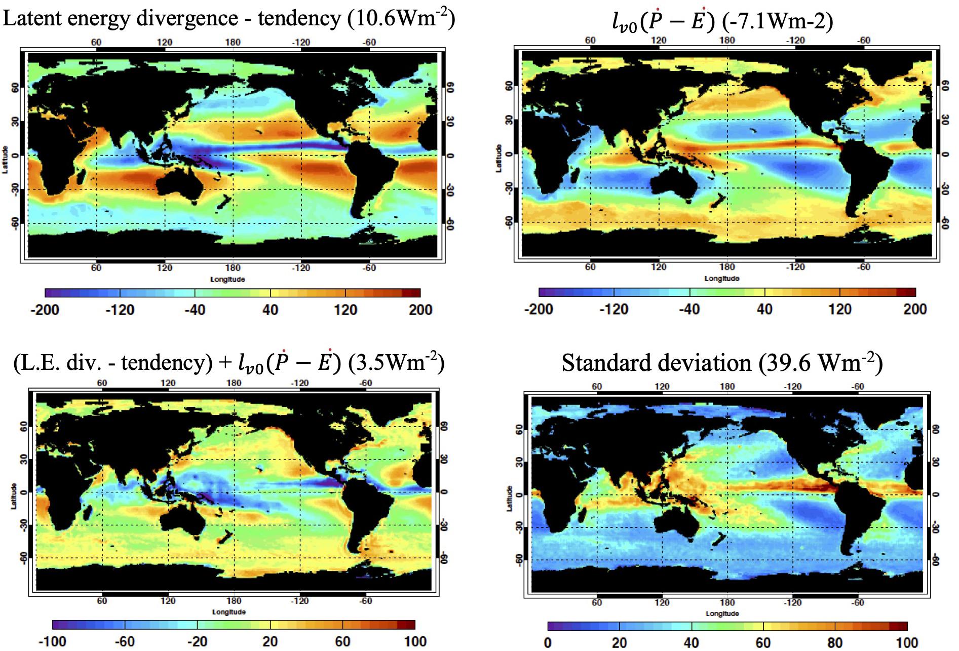
Figure 3. (Top left) Latent heat divergence plus tendency derived from ERA-Interim. (Top right) Diabatic heating by precipitation minus surface latent heat flux derived from GPCP and SeaFlux. (Bottom left) Regional water mass balance computed as latent heat divergence, tendency, and diabatic heating by precipitation minus surface latent heat flux. (Bottom right) Standard deviation of the reginal monthly water mass balance computed over 192 months. Regional values are 16-year climatological mean (from January 2001 to December 2016). Units is in Wm^{– 2} for all plots. Mean values averaged over the global ocean are shown with titles.

Because F_LH is equal to $\stackrel{.}{E}{l}_v,$Eqs. 9, and 11 suggest that a bias in the regional water mass balance can affect regional surface energy balance. In order to assess regional water mass balance, in Figure 3 we plot the divergence of water vapor as a form of the latent heat plus the tendency term on the top left panel and $l_{v0}(\stackrel{.}{P}-\stackrel{.}{E})$ on the top right panel where l_v0 is the enthalpy of vaporization at 0°C. In the tropics, water vapor converges toward the inter tropical convergence zone (ITCZ) where larger precipitation rates are present. For the atmosphere to balance water mass by Eq. 11 regionally, the sum of values shown in left and right plots needs to be 0. The bottom left plot of Figure 3 shows the water mass balance residual expressed in Wm^–2. Regions with negative values are where convergence is too large, precipitation rate is too small, or evaporation rate is too large. Although the size is unknown, the F_h term defined by Eq. 5 that are neglected in this study can contribute to both energy and water mass balance residuals (Kato et al., 2021). While the standard deviation is relatively large over the tropics (bottom right plot of Figure 3), the spatial pattern of water mass residual differs from the spatial pattern of net surface energy flux (top left panel of Figure 2). This indicates that the bias is not limited to a common component, i.e., F_LH and $l_v\stackrel{.}{E}$, which affect both balances, but also in other energy flux components likely play a role.

To understand the effect of water mass balance residual to surface net energy flux, however, we assume that all water mass residual is caused by one component of water mass fluxes. If the residual is caused by the bias in F_LH, the bias corrected F_net,c is,

where the water mass balance residual ε_M is

If the residual is caused by latent heat divergence then the bias corrected F_net,t is,

The water mass balanced surface net energy flux is F_net,c−l_v0ε_M and F_net,t−l_v0ε_M, which are shown, respectively, on the left and right panel of Figure 4. The surface net energy flux shown in Figure 4 is the flux if regional water mass were balanced. We can further combine surface net energy fluxed derived from two approaches and water mass correction to form the water mass corrected atmospheric energy balance residual,

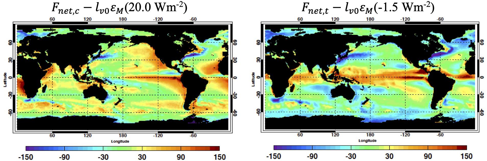
Figure 4. Water mass balanced surface net energy flux F_net,_c – l_v0ε_M given by Eq. 11 on the panel left and F_net,_t – l_v0ε_M given by Eq. 13 on the panel right. Regional values are 16-year climatological mean (from January 2001 to December 2016). Units is in Wm^{– 2} for all plots. Mean values averaged over the global ocean are shown with titles.

Figure 5 shows regional ε_E−l_v0ε_M. The bias can be associated with any of the energy flux components that appear in Eqs 9, and 10. The bias in F_LH can also contribute to ε_E−l_v0ε_M, provided that biases in water mass flux components are present in a way that the sum is not altering the regional water mass balance. Regions with a positive value need a larger upward surface energy flux or a smaller moist energy and kinetic energy divergence.

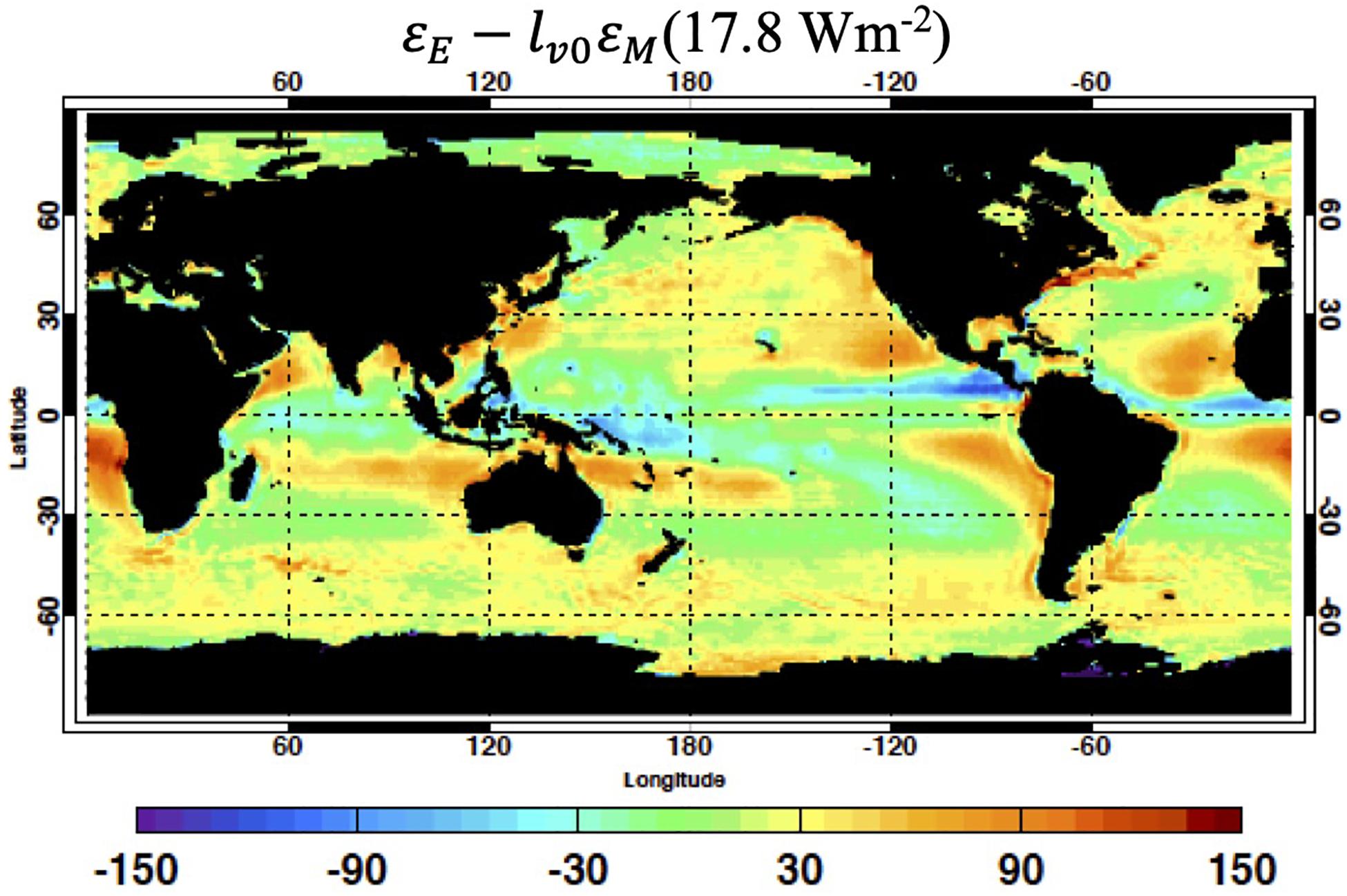
Figure 5. Water mass corrected atmospheric energy balance residual ε_E – l_v0ε_M defined by Eq. 14 in Wm^{– 2}. Mean value averaged over the global ocean is 17.8 Wm^{– 2}. Regional values are 16-year climatological mean (from January 2001 to December 2016).

Seasonal Variability

Figure 6 shows climatological seasonal variability of energy flux components averaged between 45°N and 45°S over ocean. The net TOA irradiance (blue line in the top plot) seasonal variability is similar to the seasonal variability of the climatological global mean shown in Fasullo and Trenberth (2008). The seasonal variability is largely caused by insolation driven by the Earth-to-sun distance, which in turn affects absorbed shortwave irradiance. The energy divergence in the atmosphere averaged between 45°N and 45°S over ocean is relatively constant. During May through July, the atmosphere transports more energy than net TOA irradiance, indicating that additional net energy is provided from the surface during these months. The bottom plot of Figure 6 shows the surface flux components separately. The net surface irradiance is indicated by the blue line and three estimates of turbulent flux from SeaFlux, OAFlux and ERA-Interim are indicated, respectively, by red, magenta, and green lines. In Figure 6, the net surface irradiance is positive downward and the turbulent fluxes are positive upward. From May to July, ERA-Interim turbulent flux is larger than the net irradiance, while SeaFlux and OAFlux turbulent fluxes are smaller than the net irradiance throughout the year. The larger ERA-Interim turbulent flux than the net irradiance during May through July is interpreted as the surface providing net energy to the atmosphere, which is consistent with the top plot of Figure 6. This result suggests that SeaFlux and OAFlux turbulent fluxes are too small or both the net surface irradiance and divergence are too large during these 3 months. More importantly, annual mean turbulent fluxes averaged over 45°N to 45°S over ocean derived from three different products differ by nearly 20 Wm^–2, which is approximately 14% of the annual mean value. The 20 Wm^–2 difference of turbulent fluxes is nearly equivalent to the difference between the net surface energy fluxes derived from two methods.

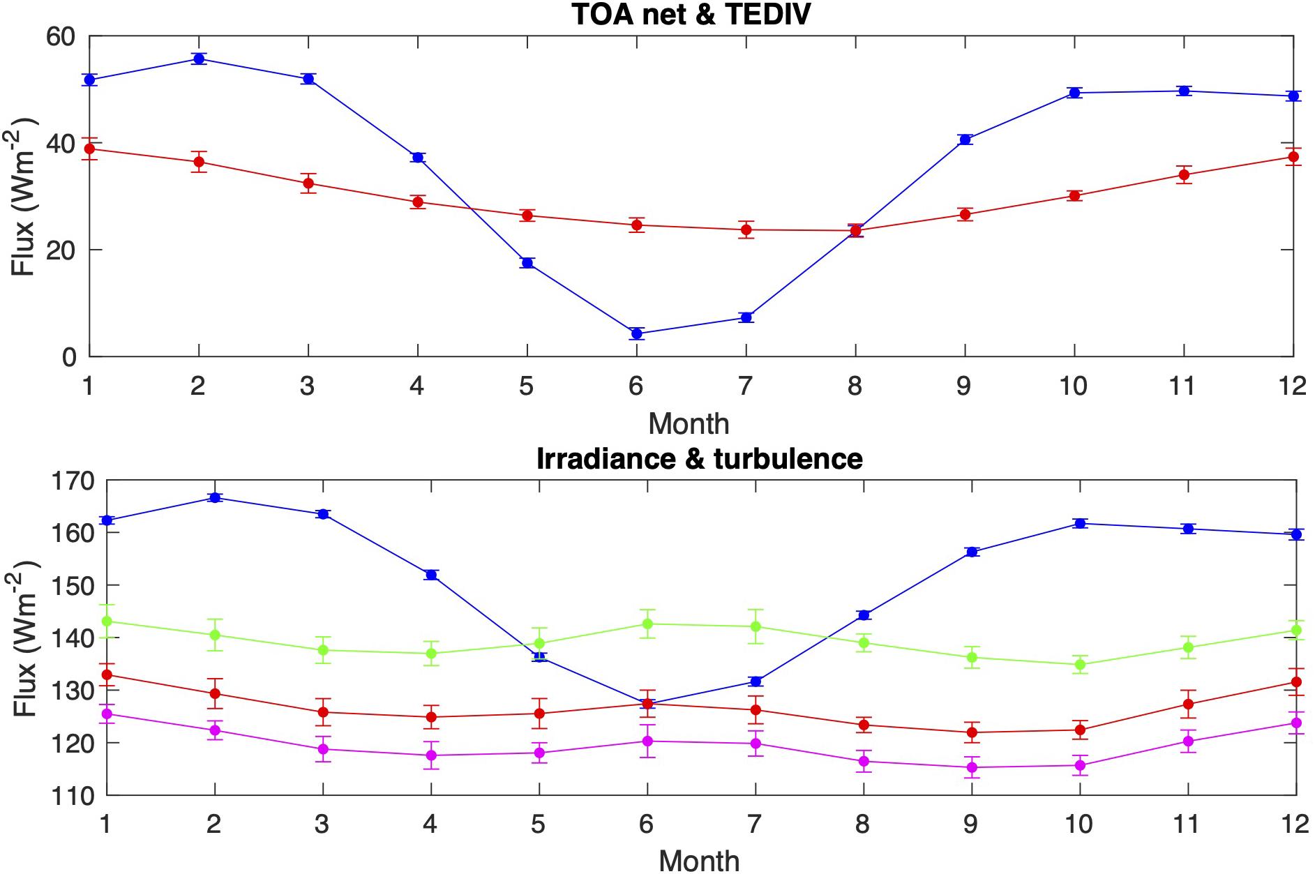
Figure 6. (Top) Climatological monthly mean net TOA irradiance (blue line) defined as positive downward and divergence of moist static and kinetic energy (red line) averaged between 45°N and 45°S over ocean. (Bottom) Net surface irradiance (blue line), turbulent flux (i.e., the sum of sensible and latent heat fluxes) derived from SeaFlux (red line), ERA-Interim (green line), and Objectively Analyzed Air-sea Fluxes (OAFlux) (magenta line). Turbulent fluxes are positive upward. Climatological means are computed with 16 years of data (January 2001 to December 2016) and error bars indicate the standard deviation.

Although the net surface energy fluxes derived by the two methods differ by more than 10 Wm^–2, Figure 6 indicates that differences of turbulent fluxes derived from ERA-Interim, SeaFlux, and OAFlux are nearly constant throughout the year. As a consequence, once respective annual mean values are subtracted, seasonal variabilities derived from two data products are similar (Figure 7, bottom plot). After the corresponding annual mean is subtracted, the difference in climatological monthly mean variability is less than ±2 Wm^–2, which is approximately 10% of the amplitude of the seasonal cycle.

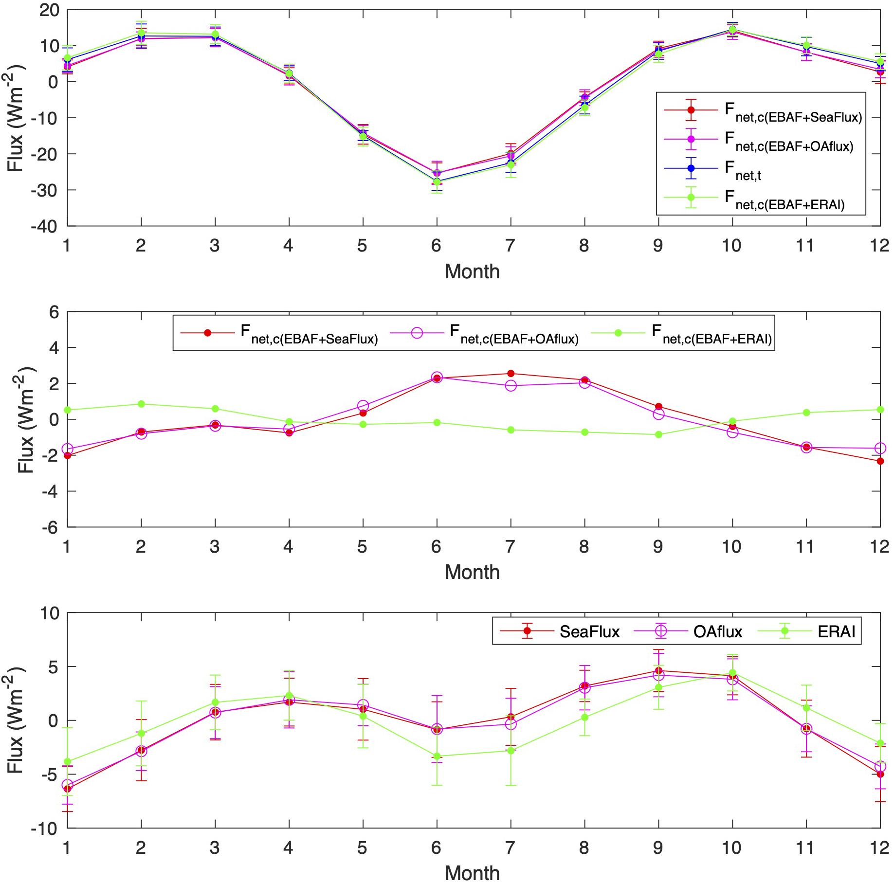
Figure 7. (Top) Monthly climatological mean of net surface energy flux variability computed by the component approach (F_net,_c) using the EBAF data product and SeaFlux (blue line), OAFLux (magenta line), and ERA-Interim (green line). Net surface energy flux computed by the transport approach (F_net,_t) is shown with red line. All values are averaged between 45°N and 45°S over ocean. Corresponding annual mean is subtracted from monthly means. Means are average from January 2001 to December 2016 and error bars indicate the standard deviation. (Middle) Difference of monthly climatological mean variabilities F_net,_c – F_net,_t, i.e., the red, magenta, and green lines minus the blue line shown in the top plot. (Bottom) Monthly mean climatology minus annual mean of sensible and latent heat fluxes computed with SeaFLux, OAFlux, and ERA-Interim products.

Discussion and Summary

Energy flux data products were integrated by two different methods to assess the regional surface energy balance. The first method is to use all surface flux components and the resulting net surface flux is denoted by F_net,c. The second method is to use the TOA net irradiance, horizontal energy transport by the atmosphere, and tendency for which the resulting net surface flux is denoted by F_net,t. While the uncertainty in regional F_net,c is larger than F_net,t, the advantage of the component approach is that it provides all components. The transport approach only provides the net surface energy flux. However, F_net,c averaged over the global ocean is 16 Wm^–2 while F_net,t averaged over the global ocean is 2 Wm^–2. The comparisons of net surface energy fluxes derived from both approaches shed lights into the uncertainties of their components. For example, the net surface energy flux averaged over global ocean is nearly equal to the ocean heating rate provided that the enthalpy transported by river runoff is negligible. Because annual mean ocean heating rate is 0.93 Wm^–2, the size of combined biases from flux components used in estimating the net surface energy flux averaged over global ocean is nearly equal to F_net,c. Our results also indicate that the residual of energy balance (16–0.93 Wm^–2) is larger than the residual of mass balance (4 Wm^–2) when they are averaged over global ocean. It is not obvious why the energy balance residual is larger than the mass balance residual. One reason might be due to the components achieving energy and mass balances. The surface energy balance is achieved largely among R_sfc, F_SH, and F_LH while the mass balance is achieved among F_LH, precipitation rate, and horizontal transport of water.

The water mass residual indirectly affects energy budget residual. Kato et al. (2021) show that regional water mass is not conserved when multiple data products are integrated. This is also illustrated in Figure 3. Horizontal transport of water vapor derived from ERA-Interim is shown on the top left plot of Figure 3. The annual mean water vapor transport from ocean to land is 4 × 10⁴ km³ yr^–1 in the units of volume, which is equivalent to 3.2 PW or approximately 10 Wm^–2. This is nearly the same size of the energy flux from ocean to land (Fasullo and Trenberth, 2008), indicating that the ocean to land energy transport is dominated by latent heat divergence. Our value of water mass divergence averaged over the global ocean in the units of energy flux of 11 Wm^–2 is consistent with the value given in Trenberth and Fasullo (2013) and Rodell et al. (2015). At a regional scale, water vapor divergence plus tendency in the atmosphere should balance with $\stackrel{.}{E}-\stackrel{.}{P}$ (Eq. 3). This implies that $\stackrel{.}{P}-\stackrel{.}{E}$ averaged over the global ocean should be approximately −10 Wm^–2, provided that the tendency term is small. When GPCP precipitation rate and SeaFlux latent heat flux are used, $\stackrel{.}{P}-\stackrel{.}{E}$ averaged over global ocean is −7 Wm^–2. This suggests that biases in $\stackrel{.}{P}$ and $\stackrel{.}{E}$ are nearly the same size and partially cancels when $\stackrel{.}{E}$ is subtracted from $\stackrel{.}{P}$. This may be the reason for the smaller water mass balance residual than the energy balance residual averaged over the global ocean. Note that the annual mean latent heat flux form OAFlux averaged over global ocean is approximately 5.5 Wm^–2 smaller than the SeaFlux counterpart value so that $\stackrel{.}{P}-\stackrel{.}{E}$ averaged over global ocean is −1.5 Wm^–2, which gives a larger ε_M than ε_M computed with SeaFlux.

The $\stackrel{.}{E}-\stackrel{.}{P}$ value also depends on precipitation data product. Generally, precipitation rate estimated over ocean is uncertain due to lack of ground-based direct observations compared to precipitation rate estimated over land (Sun et al., 2018). A study by Behrange and Song (2020) suggests that GPCP precipitation rate over global ocean is underestimated by 9%. Precipitation rates over the ITCZ regions estimated by GPCP are generally smaller than those estimated from a similar multiple observation merged global precipitation data product of the CPC Merged Analysis of Precipitation (CMAP; Xie and Arkin, 1997). In addition, GPCP precipitation over the tropics is smaller than TRMM 3B42 precipitation (Masunaga et al., 2019). In particular, heavy rain rates larger than 30 mm day^–1 over ocean occur less frequent in GPCP precipitation than TRMM 3B42v7 precipitation (Masunaga et al., 2019). The spatial pattern of water mass residual (lower left of Figure 3) suggests that the residual is not limited over the ITCZ, indicating that the water mass balance residual is not entirely caused by our choice of data products.

The surface net energy flux F_net,c averaged over the global ocean of 16 Wm^–2 is smaller than the maximum standard deviation of regional net fluxes of approximately 30 Wm^–2 derived from 12 data products shown in Yu (2019). Therefore, regional F_net,c shown in Figure 2 could change depending on the data product. Nevertheless, given the regional water vapor balance residual shown in Figure 3, the water mass balance residual contributes a large portion of the energy balance residual for some regions.

We showed that sums of latent heat and sensible heat fluxes from SeaFlux and OAFlux averaged between 45°N and 45°S over ocean during May through July are likely to be too small because the atmosphere transports energy more than energy input from the top and bottom boundary. If the moist static divergence is too large, the net surface irradiance is also too large. The difference between annual mean F_net,c and F_net,t averaged over 45°N to 45°S is 18 Wm^–2. The 20 Wm^–2 difference of turbulent fluxes found between three products is nearly equivalent to the difference of F_net,c and F_net,t. In addition, if we assume that the 2.5 Wm^–2 uncertainty in regional outgoing TOA shortwave and longwave irradiances (Loeb et al., 2018) and the 10 Wm^–2 uncertainty in horizontal transport (Trenberth and Fasullo, 2018) are independent, then the uncertainty in regional F_net,t is 11 Wm^–2 [=(2.5²+2.5²+10²)^1/2]. Therefore, the 18 Wm^–2 is likely to be larger than the uncertainty in TOA net irradiance and transport combined.

The root-mean-square (RMS) difference of monthly mean downward irradiances compared with observations at buoy sites that are mostly located in the tropics is 11 and 5 Wm^–2, respectively, for shortwave and longwave irradiances (Kato et al., 2018). The estimated uncertainty in the regional monthly mean net surface irradiance over ocean is 13 Wm^–2 (Kato et al., 2020). The uncertainty in regional turbulent flux in F_net,c is difficult to estimate. A casual comparison of latent heat flux shown in Figure 1 with the latent heat flux from the Japanese Ocean Flux Data Set with Use of Remote-sensing Observations (J-OFURO) (Figure 4 of Tomita et al., 2019) suggests that SeaFLux F_LH over tropics is smaller than Japanese ocean flux data set with use of remote-sensing observations (J-OFULO) F_LH. Comparisons of daily mean J-OFULO F_LF against buoy observations in Tomita et al. (2019) yield a typical RMS difference of less than 25 Wm^–2. If there is a random error contribution, the RMS difference in monthly means is expected to be smaller. In fact, climatological mean differences of regional F_SH and F_LH from SeaFLux and OAFlux are within 10 Wm^–2 for most regions (Figure 8), although the differences of F_SH and F_LH over tropical regions have the same sign. All these results suggest that estimated uncertainties in monthly mean R_sfc, F_SH, and F_LH are of the order of 10 Wm^–2.

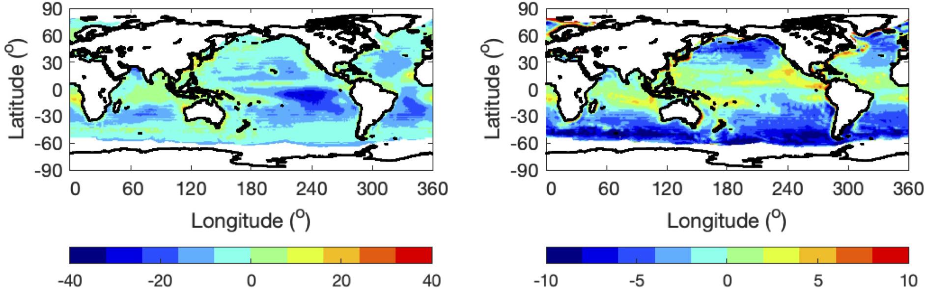
Figure 8. Difference of surface (left) latent heat flux and (right) sensible heat flux derived from OAFlux and SeaFLux data products (OAFlux minus SeaFlux) averaged over 16 years (from January 2000 to December 2015) in Wm^{– 2}. Fluxes are defined positive upward.

As mentioned in Cronin et al. (2019), the uncertainty in satellite derived gridded energy products is larger than the in situ observation uncertainty of ∼10 Wm^–2 in a long-term averaged value (e.g., monthly mean) largely due to limitations in observing surface air temperature and humidity. Near surface temperature and humidity affect both downward longwave irradiance and sensible and latent heat fluxes. In addition, ocean skin temperature retrieved from satellite observations is the temperature of the thermal skin layer of about a 0.1 mm thick below ocean surface (Wong and Minnett, 2018). Furthermore, the ocean thermal skin layer temperature is generally lower than ocean temperature below the surface at a depth of ∼2 m because of evaporative cooling at the air-sea interface (Smith et al., 1996). Therefore, satellite derived skin temperature can be different from ocean surface temperature (Cronin et al., 2019).

In addition to these input variables, there is the uncertainty associated with the turbulent flux parametrizations and the use of bulk state variables (Cronin et al., 2019; Yu, 2019). Gustiness of wind speed can alter turbulent fluxes and needs to be taken into account. Wind speed dependent ocean surface roughness length and transfer coefficients need to be improved, and their dependence on the sea state might need to be incorporated into parameterizations. Furthermore, deriving latent heat flux from satellites is challenging because of their diurnal sampling and calibration stability (Robertson et al., 2020). Also, a larger footprint size and broad passive microwave channel weighting functions are not ideal for deriving near surface humidity with a required spatial resolution (Robertson et al., 2020).

Advances in remote sensing techniques to derive surface air temperature and humidity will help reduce errors in surface irradiance. In addition, better observations of ocean surface temperature, wind speed at a high temporal resolution, and sea state at a global scale are needed to improve turbulent fluxes. Some promising observations to improve surface fluxes are proposed in Cronin et al. (2019) and are expected to provide indispensable observations toward reducing uncertainties in estimating regional surface energy fluxes. Our results highlight the weakness of the component approach to estimate regional net surface energy flux and identify regions where larger issues remain. Our analysis indicates that large surface energy flux biases exist in the tropics, which is consistent with earlier studies (Loeb et al., 2014; Kato et al., 2016). Improving future observations need to target the regions with large residuals, which could lead to improved understanding and reduction of these biases. In addition, toward achieving the goal of improving surface energy flux, data product integration and physical processes demonstrated in this study can be used to assess the quality of individual data products. Reducing surface energy budget uncertainty needs coordinate efforts among surface radiation and turbulent flux data providers.

Data Availability Statement

The datasets EBAF for this study can be found in the NASA Langley Atmospheric Science Data Center (https://ceres.larc.nasa.gov/data/), SeaFux can be found in the NASA Earthdata (https://ghrc.nsstc.nasa.gov/pub/seaflux/data/), OAFlux can be found in the Woods Hole Oceanographic Institution site (ftp://ftp.whoi.edu/pub/science/oaflux/data_v3), GPCP can be found in the University of Maryland site (http://gpcp.umd.edu/), and ERA-Interim can be found in the NCAR site (ftp://ftp.cgd.ucar.edu/archive/BUDGETS/ERAI).

Author Contributions

SK wrote the first draft of the manuscript. DP contributed to the editing. FR generated the figures. SK, FR, F-LC, DP, and WS contributed to the analysis. All authors contributed to the article and approved the submitted version.

Funding

This work was supported by the NASA CERES and the NASA’s Energy and Water cycle Study (NEWS) projects.

Conflict of Interest

FR, F-LC, and DP are employed by the company Science Systems and Applications Inc.

The remaining authors declare that the research was conducted in the absence of any commercial or financial relationships that could be construed as a potential conflict of interest.

Publisher’s Note

All claims expressed in this article are solely those of the authors and do not necessarily represent those of their affiliated organizations, or those of the publisher, the editors and the reviewers. Any product that may be evaluated in this article, or claim that may be made by its manufacturer, is not guaranteed or endorsed by the publisher.

Acknowledgments

We thank John Fasullo of NCAR for providing ERA-Interim energy transport data product and William Olson of UMBC and Brent Roberts of NASA MFSC for useful discussions.

References

Adler, R. F., Gu, G., and Huffman, G. J. (2012). Estimating climatological bias errors for the Global Precipitation Climatology Project (GPCP). J. Appl. Meteor. Climatol. 51, 84–99. doi: 10.1175/JAMC-D-11-052.1
Albrecht, B. A., Fairall, C. W., Thomson, D. W., White, A. B., and Snider, J. B. (1990). Surface-based remote sensing of the observed and the adiabatic liquid water content of stratocumulus clouds. Geophys. Res. Lett. 17, 89–92.
Behrange, A., and Song, Y. (2020). A new estimate for oceanic precipitation amount and distribution using complementary precipitation observations from space and comparison with GPCP. Environ. Res. Lett. 15:124042.
Betts, A. K. (1985). Mixing line analysis of clouds and cloudy boundary layers. J. Atmos. Sci. 42, 2751–2763.
Betts, A. K., and Ridgway, W. (1988). Coupling of the radiative convective, and surface fluxes over the equatorial Pacific. J. Atmos. Sci. 45, 522–536.
Bretherton, C. S., and Wyant, M. C. (1997). Moisture transport, lower-tropospheric stability, and decoupling of cloud-topped boundary layers. J. Atmos. Sci. 54, 148–167.
Cronin, M. F., Gentemann, C. L., Edson, J., Ueki, I., Bourassa, M., Brown, S., et al. (2019). Air-sea fluxes with a focus on heat and momentum. Front. Mar. Sci. 6:430. doi: 10.3389/fmars.2019.00430
Dee, D. P., Uppala, S. M., Simmons, A. J., Berrisford, P., Poli, P., Kobayashi, S., et al. (2011). The ERA- interim reanalysis: configuration and performance of the data assimilation system. Q.J.R. Meteorol. Soc. 137, 553–597.
Fasullo, J. T., and Trenberth, K. E. (2008). The annual cycle of the energy budget. Part I: global mean and land-ocean exchanges. J. Climate 21, 2297–2312. doi: 10.1175/2007JCLI1935.1
Hartmann, D. L., and Ceppi, P. (2014). Trends in the CERES dataset, 20000-13: the effects of sea ice and jet shifts and comparison to climate models. J. Clim. 27, 2444–2456. doi: 10.1175/JCLI-D-13-00411.1
Hersbach, H., de Rosnay, P., Bell, B., Schepers, D., Simmons, A., and Soci, C. (2018). Operational global reanalysis: progress, future directions and synergies with NWP. ERA Rep. Ser. 27:65. doi: 10.21957/tkic6g3wm
Hudson, S. R., Granskog, M. A., Sundfjord, A., Randelhoff, A., Renner, A. H. H., and Divine, D. V. (2013). Energy budget of first-year Arctic sea ice in advance stages of melt. Geophys. Res. Lett. 40, 2679–2683. doi: 10.1002/grl.50517
Jin, Z., Charlock, T. P., Smith, W. L., and Rutledge, K. (2004). A parameterization ocean surface albedo. Geophys. Res. Lett. 31:L22301. doi: 10.1029/2004GL021180
Johnson, G. C., Lyman, J. M., and Loeb, N. G. (2016). Improving estimates of Earth’s energy imbalance. Nat. Climate Change 6, 639–640. doi: 10.1038/nclimate3043
Josey, S. A., Gulev, S., and Yu, L. (2013). “Exchange through the ocean surface,” in Ocean Circulation and Climate: A 21st Century Perspective, Int. Geophys. Ser, Vol. 103, eds G. Siedler et al. (Oxford: Academic Press), 115–140.
Kato, S., Rose, F. G., Rutan, D. A., Thorsen, T. J., Loeb, N. G., Doelling, D. R., et al. (2018). Surface irradiances of edition 4.0 clouds and the earth’s radiant energy system (CERES) energy balanced and filled (EBAF) data product. J. Climate 31, 4501–4527. doi: 10.1175/JCLI-D-17-0523.1
Kato, S., Loeb, N. G., Fasullo, J. T., Trenberth, K. E., Lauritzen, P. H., Rose, F. G., et al. (2021). Regional energy and water budget of a precipitating atmosphere over ocean. J. Clim. 34, 4189–4205. doi: 10.1175/JCLI-D-20-0175.1
Kato, S., Loeb, N. G., and Rutledge, C. K. (2002). Estimate of top-of-atmosphere albedo for a molecular atmosphere over ocean using Clouds and the Earth’s Radiant Energy System measurements. J. Geophys. Res. 107:4396. doi: 10.1029/2001JD001309
Kato, S., Rose, F. G., Sun-Mack, S., Miller, W. F., Chen, Y., Rutan, D. A., et al. (2011). Improvements of top-of-atmosphere and surface irradiance computations with CALIPSO-, CloudSat-, and MODIS-derived cloud and aerosol properties. J. Geophys. Res. 116:D19209. doi: 10.1029/2011JD016050
Kato, S., Rutan, D. A., Rose, F. G., Caldwell, T. E., Ham, S.-H., Radkevich, A., et al. (2020). Uncertainty in satellite-derived surface irradiances and challenges in producing surface radiation budget climate data record. Remote Sens. 12:1950. doi: 10.3390/rs12121950
Kato, S., Xu, K.-M., Wong, T., Loeb, N. G., Rose, F. G., Trenberth, K. E., et al. (2016). Investigation of the bias in column integrated atmospheric energy balance using cloud objects. J. Clim. 29:20. doi: 10.1175/JCLI-D-15-0782.1
L’Ecuyer, T., Tristan, S., Beaudoing, H. K., Rodell, M., Olson, W., Lin, B., et al. (2015). The observed state of the energy budget in the early twenty-first century. J. Clim. 28, 8319–8346. doi: 10.1175/JCLI-D-14-00556.1
Liu, C., Allan, R. P., Berrisford, P., Mayer, M., Hyder, P., Loeb, N., et al. (2015). Combining satellite observations and reanalysis energy transports to estimate global net surface energy fluxes 1985–2012. J. Geophys. Res. Atmos. 120, 9374–9389. doi: 10.1002/2015JD023264
Liu, C., Allan, R. P., Mayer, M., Hyder, P., Desbruyeres, D., Cheng, L., et al. (2020). Variability in the global energy budget and transports 1985-2017. Clim. Dyn. 55, 3381–3396. doi: 10.1007/s00382-020-05451-8
Loeb, G. L., Thorsen, T. J., Norris, J. R., Wang, H., and Su, W. (2018). Changes in Earth’s energy budget during and after the “pause” in global warming: an observational perspective. Climate 6:62. doi: 10.3390/cli6030062
Loeb, N. G., Rutan, D. A., Kato, S., and Wang, W. (2014). Observing in- terannual variations in Hadley circulation atmospheric diabatic heating and circulation strength. J. Clim. 27, 4139–4158. doi: 10.1175/JCLI-D-13-00656.1
Masuda, K., Takashima, T., and Takayama, Y. (1988). Emissivity of pure and sea waters for the model sea surface in the infrared window regions. Remote Sens. Environ. 24, 313–329.
Masunaga, H., Schroder, M., Furuzawa, F. A., Kummerow, C., Rustemeier, E., and Schneider, U. (2019). Inter-product biases in global precipitation extremes. Environ. Res. Lett. 14:125016. doi: 10.1088/1748-9326/ab5da9
Mayer, L., Mayer, M., and Haimberger, L. (2021). Consistency and homogeneity of atmospheric energy, moisture, and mass budget in ERA5. J. Clim. 34, 3955–3974. doi: 10.1175/JCLI-D-20-0676.1
Mayer, M., Haimberger, L., Edwards, J. M., and Hyder, P. (2017). Toward consistent diagnostics of the coupled atmosphere and ocean energy budgets. J. Clim. 30, 9225–9246. doi: 10.1175/JCLI-D-17-0137.1
Meyssignac, B., Boyer, T., Zhao, Z., Hakuba, M. Z., Landerer, F. W., Stammer, D., et al. (2019). Measuring global ocean heat content to estimate the earth energy imbalance. Front. Mar. Sci. 6:432. doi: 10.3389/fmars.2019.00432
Roberts, J. B., Clayson, C. A., and Robertson, F. R. (2020). SeaFlux Data Products Version 3. Dataset Available Online from the NASA Global Hydrology Resource Center DAAC. Huntsville, AL. doi: 10.5067/SEAFLUX/DATA101
Robertson, F. R., Roberts, J. B., Bosilovich, M. G., Bentamy, A., Clayson, C. A., Fennig, K., et al. (2020). Uncertainties in ocean latent heat flux variations over recent decades in satellite-based estimates and reduced observation reanalyses. J. Clim. 33, 8415–8437. doi: 10.1175/JCLI-D-19-0954.1
Rodell, M., Beaudoing, H. K., L’Ecuyer, T. S., Olson, W. S., and Famiglietti, J. S. (2015). The observed state of the water cycle in the early twenty-first century. J. Clim. 28:8289. doi: 10.1175/JCLI-D-14-00555.1
Sidran, M. (1981). Broadband reflectance and emissivity of specular and rough water surfaces. Appl. Opt. 20, 3176–3183.
Smith, W. L., Knuteson, R. O., Revercomb, H. E., Feltz, W., Howell, H. B., Menzel, W. P., et al. (1996). Observations of the infrared radiative properties of the ocean–implications for the measurement of sea surface temperature via satellite remote sensing. Bull. Am. Meteorol. Soc. 77, 41–52.
Soden, B. J. I, Held, M., Colman, R., Shell, K. M., Kiehl, J. T., and Shields, C. A. (2008). Quantifying climate feedbacks using radiative kernels. J. Clim. 21, 3504–3520. doi: 10.1175/2007JCLI2110.1
Stephens, G. L., Li, J., Wild, M., Clayson, C. A., Loeb, N., and Kato, S. (2012). An update on Earth’s energy balance in light of the latest global observations. Nat. Geosci. 5, 691–696. doi: 10.1038/NGEO1580
Sun, Q., Miao, C., Duan, Q., Ashouri, H., Sorooshian, S., and Hsu, K.-L. (2018). A review of global precipitation data sets: data sources, estimation, and inter- comparisons. Rev. Geophys. 56, 79–107. doi: 10.1002/2017RG000574
Tomita, H., Hihara, T., Kato, S., Kubota, M., and Kutsuwada, K. (2019). An introduction to J-OFURO3, a third-generation Japanese ocean flux data set using remote-sensing observations. J. Oceanogr. 75, 171–194. doi: 10.1007/s10872-018-0493-x
Trenberth, K. E., and Fasullo, J. T. (2013). Regional energy and water cycles: transports from ocean to land. J. Climate 26, 7838–7851. doi: 10.1175/JCLI-D-13-00008.1
Trenberth, K., and Fasullo, J. (2018). Applications of an updated atmospheric energetics formulation. J. Clim. 31, 6263–6279. doi: 10.1175/JCLI-D-17-0838.1
Trenberth, K. E. (1991). Climate diagnostics from global analysis: conservation of mass in ECMWF analysis. J. Clim. 4, 707–722.
Trenberth, K. E. (1997). Using atmospheric budgets as constraint on surface fluxes. J. Clim. 10, 2796–2809.
Trenberth, K. E., Caron, J. M., and Stepaniak, D. P. (2001). The atmospheric energy budget and implications for surface fluxes and ocean heat transports. Clim. Dyn. 17, 259–276.
Trenberth, K. E., and Solomon, A. (1994). The global heat balance: heat transport in the atmosphere and ocean. Clim. Dyn. 10, 107–134.
Trenberth, K. E., and Stepaniak, D. P. (2004). The flow of energy through the earth’s climate system. Q. J. R. Meteorol. Soc. 130, 2677–2701.
von Schuckmann, K., Cheng, L., Palmer, M. D., Hansen, J., Tassone, C., Aich, V., et al. (2020). Heat stored in the earth system: where does the energy go? Earth Syst. Sci. Data 12, 2013–2041. doi: 10.5194/essd-12-2013-2020
Wild, M., Folini, D., Hakuba, M. Z., Schar, C., Seneviratne, S. I., Kato, S., et al. (2015). The energy balance over land and oceans: an assessment based on direct observations and CMIP5 climate models. Clim. Dyn. 44, 3393–3429.
Wong, E. W., and Minnett, P. J. (2018). The response of the ocean thermal skin layer to variations in incident infrared radiation. J. Geophys. Res. Oceans 123, 2475–2493.
Wood, R. (2012). Stratocumulus clouds. Monthly Weather Rev. 140, 2373–2423. doi: 10.1175/MWR-D-11-00121.1
Xie, P., and Arkin, P. A. (1997). Global precipitation: a 17-year monthly analysis based on gauge observations, satellite estimates, and numerical model outputs. Bull. Am. Meteor. Soc. 78, 2539–2558.
Yu, L. (2019). Global air–sea fluxes of heat, fresh water, and momentum: energy budget closure and unanswered questions. Annu. Rev. Mar. Sci. 11, 227–248. doi: 10.1146/annurev-marine-010816-060704
Yu, L., and Weller, R. A. (2007). Objectively analyzed air-sea heat Fluxes (OAFlux) for the global ocean. Bull. Am. Meteorol. Soc. 88, 527–539.
Yu, L., Jin, X., and Weller, R. A. (2008). Multidecade Global Flux Datasets from the Objectively Analyzed Air-Sea Fluxes (OAFlux) Project: Latent and Sensible Heat Fluxes, Ocean Evaporation, and Related Surface Meteorological Variables. Woods Hole Oceanographic Institution, OAFlux Project Technical Report. OA-2008-01. Massachusetts: Woods Hole, 64.
Keywords: energy budget, climatology, ocean surface, remote sensing, atmosphere-ocean coupling
Citation: Kato S, Rose FG, Chang F-L, Painemal D and Smith WL (2021) Evaluation of Regional Surface Energy Budget Over Ocean Derived From Satellites. Front. Mar. Sci. 8:688299. doi: 10.3389/fmars.2021.688299
Received: 30 March 2021; Accepted: 16 August 2021;
Published: 06 September 2021.
Edited by:
Meghan F. Cronin, Pacific Marine Environmental Laboratory, National Oceanic and Atmospheric Administration (NOAA), United StatesReviewed by:
Samson Hagos, Pacific Northwest National Laboratory (DOE), United StatesChunlei Liu, Guangdong Ocean University, China
Copyright © 2021 Kato, Rose, Chang, Painemal and Smith. This is an open-access article distributed under the terms of the Creative Commons Attribution License (CC BY). The use, distribution or reproduction in other forums is permitted, provided the original author(s) and the copyright owner(s) are credited and that the original publication in this journal is cited, in accordance with accepted academic practice. No use, distribution or reproduction is permitted which does not comply with these terms.
*Correspondence: Seiji Kato, seiji.kato@nasa.gov