Toward Determining the Spatio-Temporal Variability of Upper-Ocean Ecosystem Stoichiometry From Satellite Remote Sensing
 Tatsuro Tanioka
 Cédric G. Fichot
 Katsumi Matsumoto
- 1Department of Earth and Environmental Sciences, University of Minnesota, Minneapolis, MN, United States
- 2Department of Earth and Environment, Boston University, Boston, MA, United States
The elemental stoichiometry of particulate organic carbon (C), nitrogen (N), and phosphorus (P) connects the C fluxes of biological production to the availability of the limiting nutrients in the ocean. It also influences the marine food-web by modulating zooplankton’s feeding behavior and organic matter decomposition by bacteria. Despite its importance, there is a general paucity of information on how the global C:N:P ratio evolves seasonally and interannually, and large parts of the global ocean remain devoid of observational data. Here, we present a new method combining satellite ocean-color data with a cellular-trait-based model to characterize the spatio-temporal variability of the phytoplankton stoichiometry in the surface mixed layer of the ocean. This new method is demonstrated specifically for the C:P ratio. The approach was applied to phytoplankton growth rates and chlorophyll-to-carbon ratios derived from MODIS-Aqua and maps of temperature-dependent nutrient limitation to generate global and seasonal maps of upper-ocean phytoplankton C:P. Taking it a step further, we determined the C:P of the bulk particulate organic matter, using MODIS-Aqua estimates of particulate organic carbon and phytoplankton biomass. Our results are within 95% confidence interval of available data for both horizontal distributions and time series, indicating our new method’s viability in accurately quantifying seasonally resolved global ocean bulk C:P. We anticipate the new hyperspectral capabilities of the NASA PACE (Plankton, Aerosol, Cloud, ocean Ecosystem) mission will facilitate the determination of phytoplankton stoichiometry for different size classes and further enhance the predictability of marine-ecosystem stoichiometry from space.
Introduction
Ever since Redfield first reported on the C:N:P ratio of particulate organic matter (POM) more than 85 years ago (Redfield, 1934), the ratio has been widely assumed to be stable. A fixed C:N:P ratio has long played a central role in ocean biogeochemistry because this ratio largely determines the strength of the biologically mediated ocean carbon cycle. However, recent studies show convincingly that the C:N:P stoichiometry of POM varies substantially on ocean-basin scales. For example, Martiny et al. (2013a) showed a globally coherent pattern, with C:N:P ratio of 195:28:1 in the subtropical gyres, 137:18:1 in the warm upwelling zones, and 78:13:1 in the nutrient-rich polar regions. An inverse model of ocean biogeochemistry also inferred a similar spatial pattern of the global C:P and N:P ratios (Teng et al., 2014; Wang et al., 2019).
As carbon export is inversely related to atmospheric CO2 (Volk and Hoffert, 1985), carbon-enriched particulate organic matter in subtropical gyres could lead to lower atmospheric CO2 and higher export production of carbon, thereby influencing climate (Galbraith and Martiny, 2015; Tanioka and Matsumoto, 2017; Matsumoto et al., 2020a; Ödalen et al., 2020). The ocean carbon modeling community is beginning to respond to this development. For example, the state of the art CMIP5/6 models developed by various climate modeling teams around the world represent phytoplankton stoichiometry with varying degree of flexibility, from no flexibility (i.e., fixed C:N:P ratio) to fully flexible (e.g., Bopp et al., 2013; Arora et al., 2020).
A major challenge to adopting fully flexible stoichiometry in biogeochemical models is our current inability to observationally constrain the temporal variability of the C:N:P in the global ocean. Although some progress has been made to explore a temporal shift in C:N:P using local time-series data (Hebel and Karl, 2001; Karl et al., 2001; Singh et al., 2015; Martiny et al., 2016; Talarmin et al., 2016), our holistic global view of the global C:N:P ratio variation is still unclear. In situ C:N:P measurements of POM inherently suffer from bias toward regions and periods of active oceanographic research, and large parts of the global ocean remain devoid of data. For example, there is a considerable paucity of POM sampling efforts in the South and Equatorial Atlantic regions (Sharoni and Halevy, 2020).
Satellite ocean-color sensors have the potential to provide a unique tool to constrain the temporal evolution of organic matter C:N:P ratio. Ocean color provides global, synoptic views of the spectral remote-sensing reflectance of the ocean that can be used to generate estimates of marine inherent optical properties (IOPs) at various timescales (Werdell et al., 2018). Satellite ocean color (i.e., remote-sensing reflectance) provides an unparalleled tool to capture climate-driven signals in the upper biological functions of the global ocean (Dierssen, 2010; Dutkiewicz et al., 2019), and has the potential to yield crucial information on the modes of C:N:P variability. Previous field studies have shown that C:N:P ratio is significantly influenced by interannual climate variabilities such as ENSO and Pacific Decadal Oscillation (Martiny et al., 2016; Fagan et al., 2019).
One possible approach to assess the spatio-temporal variability in the C:N:P of POM is to directly estimate the change in the total concentration of particulate organic carbon (POC), particulate organic nitrogen (PON), and particulate organic phosphorus (POP) using satellite ocean color data. Multiple methods of estimating total POC from satellite ocean color have been developed over the years, and the satellite estimates are extensively calibrated with in situ measurements (Evers-King et al., 2017; Rasse et al., 2017). More recently, Fumenia et al. (2020) have developed a method to link the backscattering coefficient (bbp) at 700 nm with PON and POP concentrations in the oligotrophic Western Tropical South Pacific. However, the reliability of bbp as a quantitative proxy of PON and POP still needs to be investigated in other oceanographic areas, including non-oligotrophic regions.
Another possible approach of deriving C:N:P of bulk POM is to predict phytoplankton’s elemental composition and use it as a proxy for the bulk composition, assuming phytoplankton makes up the largest proportion of POM. The study by Arteaga et al. (2014) showed a seasonally variable global C:N:P ratio of phytoplankton by using a combination of remote sensing data and a mechanistic growth-model of phytoplankton (Pahlow et al., 2013). More recently, Roy (2018) developed a method to estimate the macromolecular content of phytoplankton protein, carbohydrate, and lipid via satellite ocean color by using empirical relationships between the particulate backscattering coefficient, phytoplankton cell size, and cellular macromolecular concentrations. However, this method cannot derive phytoplankton C:P as there is no empirical link between cell size and P-rich macromolecules such as RNA and DNA (Finkel et al., 2016; Tanioka and Matsumoto, 2020b). Furthermore, a fundamental limitation in both of these studies is that the elemental composition of phytoplankton may not be able to explain the full dynamics of bulk POM because, in reality, phytoplankton biomass typically constitute only 30–50% of bulk particulate organic matter in the open ocean (Eppley et al., 1992; Durand et al., 2001; Gundersen et al., 2001; Behrenfeld et al., 2005).
Here, we propose a new remote-sensing approach that uniquely combines established methodologies in order to quantify the spatio-temporal variability of the upper-ocean stoichiometry of phytoplankton and bulk POM (Figure 1). We demonstrate that this method specifically for the C:P ratio as C:P is more commonly compared to observations than C:N and N:P under different environmental conditions (e.g., Sterner et al., 2008). Furthermore, the C:P is a key variable for converting phosphorus-based fluxes to carbon-based fluxes in biogeochemical models, and therefore has important implications for the carbon cycle (e.g., Matsumoto et al., 2020b). The framework, however, can theoretically be expanded to include C:N and N:P ratios. In this approach, we first determine C:P of phytoplankton by combining satellite-derived estimates of growth rate, Chl:C ratio, and nutrient depletion temperatures (NDTs) with a newly developed mechanistic model of phytoplankton stoichiometry (Inomura et al., 2020). We then convert phytoplankton C:P ratio to the total POC:POP using remotely sensed concentrations of phytoplankton biomass and POC. This approach is unique in that all inputs are derived from satellite remote sensing and does not rely on in situ measurements, thereby enabling us to predict the “real-time” evolution of phytoplankton and bulk POM C:P on various temporal and spatial scales of interest.
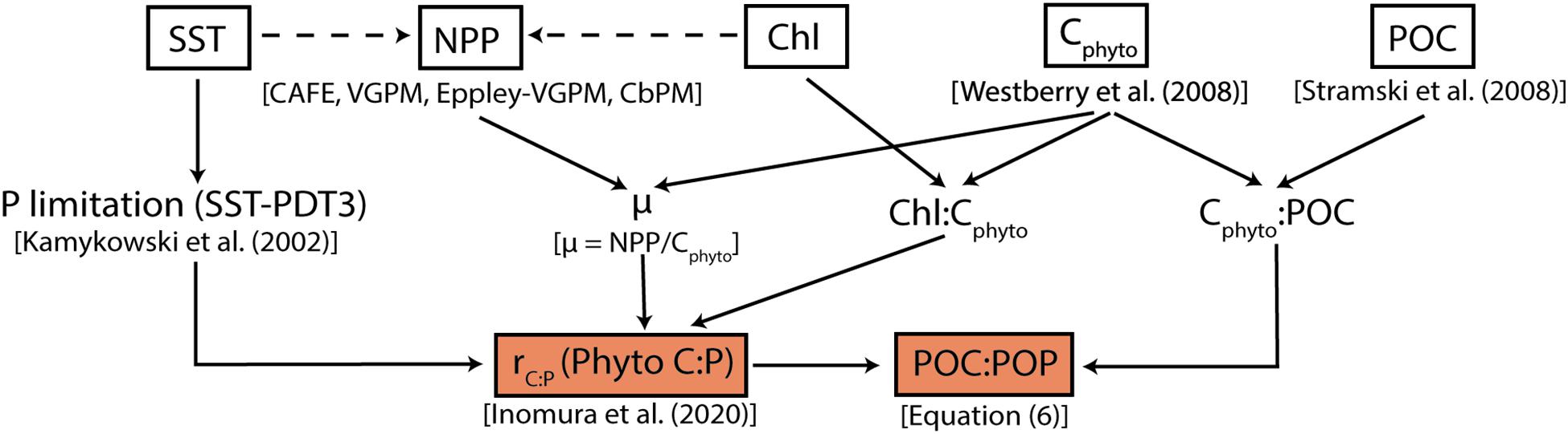
Figure 1. Flowchart summarizing the modeling framework. White squares represent globally gridded data from MODIS-Aqua and their direct products (NPP, Cphyto, and POC). The dashed arrows pointing toward NPP indicate that remotely sensed SST and Chl are used in deriving NPP. Orange boxes are main products from this study; C:P of phytoplankton (rC:P) and bulk POC:POP.
The relative importance of the two main drivers of POC:POP variability are discussed following their (1) variability due to change in phytoplankton C:P that reflect changes in environmental condition such as nutrient supply (e.g., Martiny et al., 2013a; Garcia et al., 2018), and (2) variability due to change in community plankton composition (e.g., Weber and Deutsch, 2010; Talmy et al., 2016; Sharoni and Halevy, 2020). Finally, we discuss caveats, limitations, and future directions. Our ultimate goal in this paper is to demonstrate the method’s feasibility, given all the assumptions and limitations. We envision that future advances in satellite instrumentation will enhance the accuracy of satellite-derived input parameters and improve the overall estimate of C:N:P from space.
Materials and Methods
Satellite-Informed Modeling Framework
The flowchart shown in Figure 1 provides an overview of how we determine phytoplankton C:P and bulk POC:POP ratios from satellite products. In the sections below, we briefly describe the phytoplankton stoichiometry model and the method of estimating the bulk C:P of POM.
Phytoplankton Stoichiometry Model
In this study, we determined the C:P ratio for a single phytoplankton functional type using a recently developed phytoplankton stoichiometry model (Inomura et al., 2020). The phytoplankton stoichiometry model of Inomura et al. (2020) is conceptually simple but facilitates the accurate computation of phytoplankton C:P and C:N ratios under a variety of environmental conditions. The input variables required in calculating phytoplankton C:P are light intensity, growth rate, and the presence/absence of limiting nutrients. The model is based on four empirically supported lines of evidence: (1) a saturating relationship between light intensity and photosynthesis, (2) a linear relationship between RNA-to-Protein ratio and growth rate, (3) a linear relationship between biosynthetic proteins and growth rate, and (4) a constant macromolecular composition of the light-harvesting machinery. Also, it follows from these assumptions that chlorophyll-to-carbon ratio (Chl:Cphyto) and growth rate are directly linked for any given light intensity (Laws and Bannister, 1980). Inomura et al. (2020) calibrated their model parameters subject to constraints from published laboratory chemostat studies for several key prokaryotic and eukaryotic phytoplankton species. For this study, we used the model parameter set for the cyanobacteria Synechococcus linearis because the parameters for this species were most rigorously calibrated with laboratory data compared to the other two possible options (cf. a diatom, Skeletonema costatum, and a haptophyte, Pavlova lutheri). Also, picocyanobacteria such as Synechococcus and Prochlorococcus are the most abundant phytoplankton types in the global ocean (Flombaum et al., 2013; Berube et al., 2018). Thus, if we are choosing a single group of phytoplankton to represent the whole phytoplankton community, as we do in this study, Synechococcus would be a reasonable choice. However, as this particular species of Synechococcus is a freshwater species, further calibration efforts specific to the marine cyanobacteria species would be necessary. Although the ecology of marine and freshwater phytoplankton is fundamentally similar (Kilham and Hecky, 1988), a previous meta-analysis study has shown that the interactive effects of multiple environmental stressors (e.g., temperature, light, and nutrients) on C:N:P may be significantly different for marine and freshwater species (Villar-Argaiz et al., 2018). A complete description and evaluation of the phytoplankton stoichiometry model are provided in the original model description paper (Inomura et al., 2020).
In order to determine phytoplankton C:P, we made three minor modifications to the original stoichiometry model by Inomura et al. (2020). First, we drove the stoichiometry model directly with depth-integrated Chl:Cphyto in the mixed layer obtained from the satellite ocean color instead of calculating Chl:Cphyto as a function of photon-flux density. This way, we could circumvent the need to estimate depth-dependent irradiance, which is complicated by issues such as self-shading and particle scattering (Jamet et al., 2019). Second, we imposed a fixed maximum growth rate of 2 d–1 in calculating C:P, which is equal to the maximum growth rate commonly imposed on the satellite-based estimates of growth rate (Westberry et al., 2008; Laws, 2013). Third, we imposed a constant C:P value of 102 under the P-replete condition regardless of the P supply. A C:P of 102 corresponds to the maximum capacity of cellular P (), and was used in the original stoichiometry model by Inomura et al. (2020). This assumption for Synechococcus is supported by culture experiments (e.g., Healey, 1985) and makes it possible to circumvent the need to calculate C:P based on the absolute values of external nutrient supply. Under P limitation, all cellular P tends to be allocated toward DNA, RNA, and phospholipids in the thylakoid membranes. Therefore, by default, the stoichiometry model does not require information on external nutrient concentration in calculating cellular C:P. With these three modifications, we were able to predict phytoplankton C:P using only satellite ocean color products as inputs.
Satellite-Derived Inputs
We drove the modified Inomura model with satellite-derived phytoplankton growth rates (μ), Chl:Cphyto (a measure of light intensity), and P limitation [as the difference between Sea Surface Temperature (SST) and cubic root-corrected phosphate depletion temperature (PDT3)] to estimate phytoplankton C:P (rC:P) in the surface mixed layer (Eq. 1):
The required input data in Eq. 1 are monthly binned and averaged observations from the Aqua Moderate Resolution Imaging Spectroradiometer (MODIS-Aqua) acquired from January 2003 to December 2018 and re-gridded on a regular 1°-latitude by 1°-longitude grid. All satellite-derived input data and estimates of mixed-layer depth are available for download from the Oregon State Ocean Productivity Website1.
The carbon-based specific growth rate μ (measured in d–1) is estimated by dividing the depth-integrated net primary productivity (NPP, measured in mg C m–2 d–1) by the standing stock of phytoplankton carbon (Cphyto, measured in mg C m–2):
Growth rate is influenced by light, temperature, and nutrient availability, and previous culture measurements (e.g., MacIntyre et al., 2002) provide robust and well-understood empirical relationships between μ and satellite products (Silsbe et al., 2016). There are multiple NPP data products available to date (Westberry and Behrenfeld, 2014; Bisson et al., 2018). In order to illustrate the robustness of our C:P determination to the choice of the NPP products, we used the following four NPP satellite data products: (1) the Carbon, Absorption and Fluorescence Euphotic-resolving model (CAFE) (Silsbe et al., 2016), (2) the Vertically Generalized Productivity Model (VGPM) (Behrenfeld and Falkowski, 1997), (3) the Eppley-VGPM Model (Eppley, 1972; Behrenfeld and Falkowski, 1997), and (4) the Carbon-based Productivity Model (CbPM) (Westberry et al., 2008). A previous study showed that CAFE compares best with in situ NPP measurements (Bisson et al., 2018). Because the growth rates from VGPM, Eppley-VGPM, and CbPM are similar quantitatively (Supplementary Figure 1), we only present results from VGPM as representing the three models in the main text. Throughout the text, we use the phrases “CAFE-informed phytoplankton C:P” and “VGPM-informed phytoplankton C:P” to refer to C:P calculated using μ from CAFE-based NPP and VGPM-based NPP, respectively.
For Cphyto, the satellite data product of Westberry et al. (2008) was used, who computed Cphyto as a linear function of the particulate backscatter coefficient at 443 nm, bbp(443). We only considered a single algorithm of Cphyto in this study because the previous intercomparison study showed that no single algorithm outperforms any of the other algorithms when compared with in situ data (Martínez-Vicente et al., 2017). We excluded from our analyses the coastal regions with Cphyto exceeding 1,000 mg C m–3 and we multiplied the monthly mean surface concentration of Cphyto with monthly mean mixed layer depth (MLD) from the Hybrid Coordinate Ocean Model (HYCOM) to get the depth-integrated Cphyto. Here, MLD is defined as the depth where the density of water is greater than that of water at a reference depth of 10 m by 0.125 kg m–3 (Levitus, 1982). The growth rate calculated this way in Eq. 2 is representative of a well-mixed, photoacclimated community subject to the median PAR in the mixed layer. The satellite-derived seasonal variability in μ reflect changes in light and nutrient limitation, as well as phytoplankton community composition (Behrenfeld et al., 2005).
Supplementary Figure 1 shows satellite-derived estimates of μ during summer and winter. CAFE predicts a higher μ during summer months compared to winter months for the large parts of the ocean (Supplementary Figures 1A–C). VGPM and the other two NPP products (CbPM and Eppley-VGPM) show similar trends at high latitudes but show the opposite trend in the subtropics with lower μ during summer compared to winter. As a result, the range of estimated μ amongst NPP products are higher during the summer compared to winter and is most extensive in the subtropics. Throughout the rest of this paper, the “summer” average refers to average values during July–September in the Northern Hemisphere and January–March in the Southern Hemisphere. For the “winter,” the target months are reversed between two hemispheres.
The Chl:Cphyto ratio, a proxy for light limitation (Falkowski et al., 1985; MacIntyre et al., 2002), is computed here by dividing MODIS-derived Chl-a with Cphyto. Chl-a concentration is depth-integrated and therefore converted from mg Chl m–3 to mg Chl m–2 by multiplying the monthly mean surface concentration with monthly mean MLD. Like for growth rate, Chl:Cphyto is assumed to be vertically uniform in the mixed layer. Considering ocean-color measurements are typically representative of the first optical depth of the surface ocean (Volpe et al., 2012; Bellacicco et al., 2018), this assumption is widely used in satellite remote sensing models, including the four NPP models used here. However, this assumption overlooks depth-dependent changes in Chl:Cphyto, for example when the deep chlorophyll maximum (DCM) becomes much shallower than the mixed layer depth (Cullen, 1982). Supplementary Figures 2A–C shows estimates of Chl:Cphyto during summer and winter. In general, Chl:Cphyto is higher during winter than summer as the reduced incident irradiance causes phytoplankton to allocate more of the cellular component to the light-harvesting apparatus (Geider, 1987; MacIntyre et al., 2002; Arteaga et al., 2016). High Chl:Cphyto in the sunlit layer of the continental margins are known to be relatively inaccurate and biases due to interferences by the high and variable amounts of colored dissolved organic matter (CDOM) and detritus (Siegel et al., 2005; Morel and Gentili, 2009; Loisel et al., 2010). As we excluded coastal regions in the subsequence analyses, this issue should not affect our satellite-informed C:P estimates.
P limitation was assessed by utilizing nutrient depletion temperatures (NDTs), which are temperatures above which nutrients are no longer detectable by traditional wet-chemistry techniques (Zentara and Kamykowski, 1977; Kamykowski and Zentara, 1986). The method leverages an observed inverse empirical relationship between surface nutrient concentration and sea-surface temperature (SST). In this relationship, phytoplankton is considered nutrient-limited if the difference between SST and NDT is higher than 0 and vice versa if the difference is lower than 0. We used a global NDT mask of the percentile-based, cubic root-corrected phosphate depletion temperatures (PDT3) re-gridded to a 1-by-1° spatial resolution (Supplementary Figure 2F; Kamykowski et al., 2002). PDT3 was subtracted from MODIS-derived monthly mean SST to determine the absence/presence of P limitation in the surface ocean. P limitation as a result of SST exceeding phosphate depletion temperature is globally prevalent during summer (Supplementary Figure 2D). Phosphate depletion is alleviated during winter months at high latitudes and in some parts of the equatorial regions as the surface ocean cools in part because of enhanced vertical mixing (Supplementary Figure 2E). For the current work, we limited our study to latitudes ranging from 50°S to 70°N as the original data on PDT3 beyond this latitudinal range are sparse (Kamykowski et al., 2002). We further discuss the caveats and limitations of this approach in section “Caveats, Limitations, and Future Needs.”
MODIS-derived total monthly averaged POC (0.7 μm < D < 17 μm) was obtained from the NASA Ocean Color Product webpage2. This total POC determination is based on an empirical relationship between POC and the blue-to-green band of spectral remote-sensing reflectance (Stramski et al., 2008). The algorithm employed here is widely implemented for producing maps of surface POC. The global mean Cphyto:POC is ∼30% (Supplementary Figures 2G,H), consistent with previous estimates (Behrenfeld et al., 2005). The Cphyto:POC is generally higher in the subtropical gyres than other regions reaching up to 50–70% during summer (Supplementary Figure 2G). Cphyto:POC ratio rarely exceeds a value of 1 except during episodic events in coastal regions, which we disregard in our analyses. Although Cphyto and POC are independently determined, the fact that Cphyto:POC ratio rarely exceeds a value of 1 increases our confidence in the predictability of Cphyto:POC.
Estimating C:P of Bulk POM
Globally, phytoplankton-derived organic matter represents on average ∼30% of bulk organic matter (Eppley et al., 1992; Durand et al., 2001; Gundersen et al., 2001; Behrenfeld et al., 2005), and the rest is due to contributions from zooplankton and non-living detrital materials. A previous satellite-based study showed that phytoplankton carbon biomass makes up 30–70% of the total POC pool in the tropical oligotrophic regions and ∼10–30% in higher latitudes and equatorial Pacific (Arteaga et al., 2016). The relative contribution from phytoplankton biomass is lower in nutrient-rich regions, possibly due to the top-down control on phytoplankton biomass by zooplankton (Ward et al., 2014; Talmy et al., 2016), resulting in higher zooplankton fraction and smaller phytoplankton fraction in the total POC pool.
In order to estimate C:P of bulk POM, we split the POC and particulate organic phosphorus (POP) into two components: (1) phytoplankton-derived organic matter with C:P ratio following the stoichiometry model in the previous section, and (2) non-algal component with fixed C:P of 117:1 following Anderson and Sarmiento (1994). Throughout the rest of this paper, the “community composition” refers to the relative balance between the algal and non-algal components of organic matter, not the community composition of different phytoplankton functional types.
The non-algal component of particulate organic matter with fixed C:P represents a combination of zooplankton and other non-living detrital materials such as fecal pellets and other organic matter left over from sloppy feeding (Martiny et al., 2013a, b; Talmy et al., 2016). Previous studies have shown that zooplankton generally has a C:P close to the Redfield ratio even under P-limited conditions (e.g., Copin-Montegut and Copin-Montegut, 1983; Sterner and Elser, 2002). Isopycnal analysis of export and remineralization stoichiometry of the deep ocean (>400 m) also indicates a relatively constant C:P of around ∼117 globally (Anderson and Sarmiento, 1994).
In calculating the C:P ratio of bulk POM, we solve for three unknowns: (1) the carbon content of non-algal POM (Cnon), (2) the phosphorus content of non-algal POM (Pnon), and (3) total POP. This is achieved with three equations:
The subscript “phyto” refers to the phytoplankton component, and “non” refers to the non-algal component of POM. All the quantities are in mol per unit volume. Eqs 3 and 4 describe the conservation of carbon and phosphorus, respectively, and the Eq. 5 describes the fixed C:P ratio of non-algal organic matter. Essentially, Eqs 3–5 constitute a simple two end-member mixing model of the algal and non-algal components. We can obtain C:P of the bulk organic matter as a function of the known quantities from section “Satellite-Informed Modeling Framework,” Cphyto, rC:P, and total POC by rearranging Eqs 1, 3–5:
Eq. 6 shows that the bulk C:P ratio is a non-linear function of phytoplankton C:P (rC:P) and the relative abundance of Cphyto over total POC (Cphyto/POC).
Model-Data Comparison of POC:POP
We compared the satellite-informed bulk POC:POP with a recently compiled data set of 5573 in situ observations of suspended oceanic POC:POP ratios from cruises and other marine stations distributed globally (Martiny et al., 2014). The suspended POM samples were collected on 0.7 μm filters (GF/F), and their C:P ratios reflect contributions from phytoplankton, microzooplankton, detrital material, and mixed particle aggregates. We note that the nominal pore size of 0.7 μm cannot fully capture biomass of small bacterioplankton cells (Lee and Fuhrman, 1987; Gundersen et al., 2001), which typically have C:N:P close to the Redfield Ratio (Gundersen et al., 2002). Here, we only used samples from the upper 100 m of the water column, representative of an average mixed layer (Kara et al., 2003) and excluded samples with POP concentrations inferior to the reported detection limit of 5 nM. We also removed samples from coastal waters, which often include a substantial contribution of allochthonous POM (e.g., benthic, riverine) (Liénart et al., 2018).
When comparing the large-scale temporal variability of in situ C:P with satellite estimates, we binned the measured C:P data into 10°-latitude increments. At each sampling station, we calculated the mean C:P in the top 100 m. After this screening process, we were left with 185 observational points for summer and 111 observational points for winter (Figure 2). We compared the seasonally averaged, satellite-informed POC:POP with the C:P of suspended POM spanning from 50°S to 70°N.
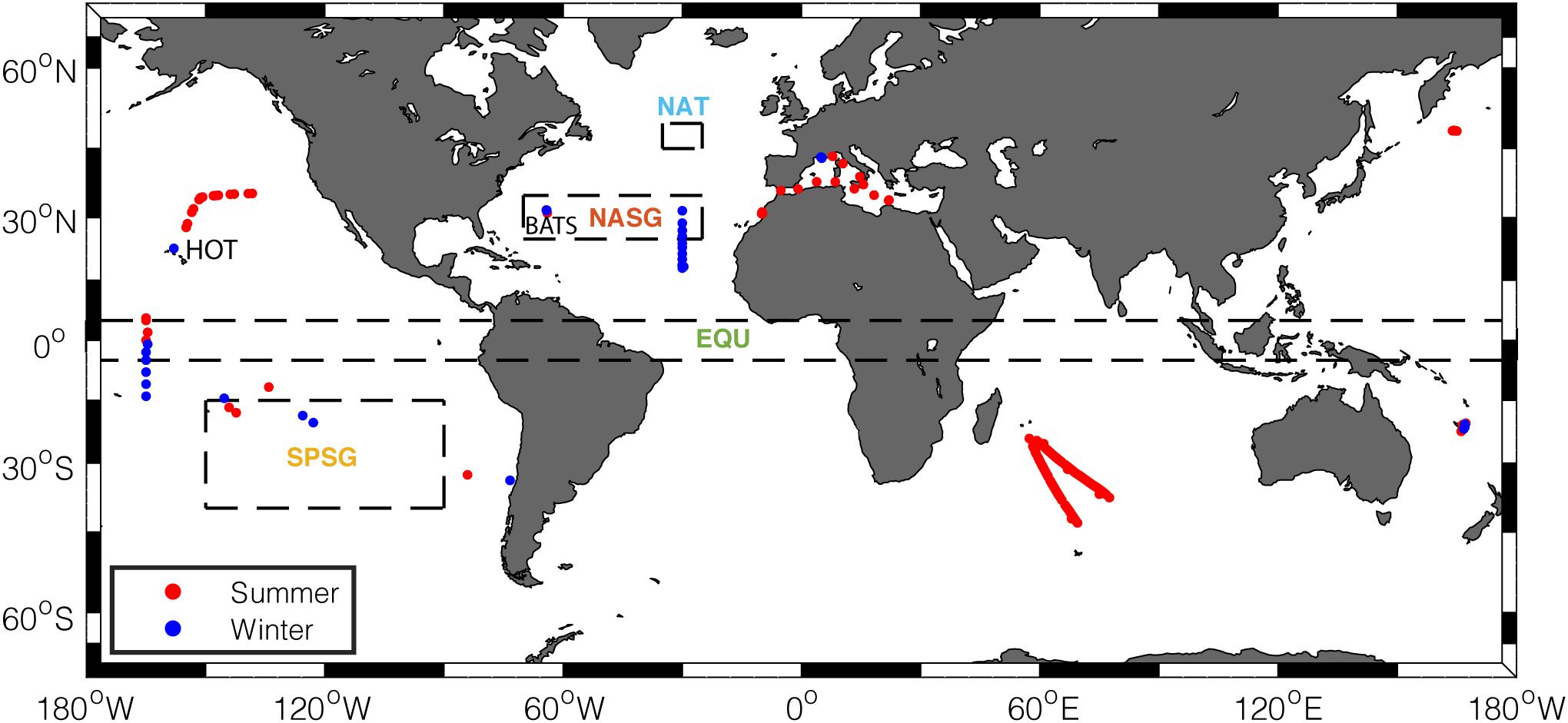
Figure 2. Geographical locations of suspended POM sample stations used in this study. Red dots represent samples collected in summer months (July–September in the Northern Hemisphere, January–March in the Southern Hemisphere), and blue dots represent samples collected in winter months (January–March in the Northern Hemisphere, July–September in the Southern Hemisphere). Dashed boxes delineate regions where the seasonality of satellite-informed estimate is examined (NAT, North Atlantic Temperate; NASG, North Atlantic Subtropical Gyre; SPSG, South Pacific Subtropical Gyre; EQU, Equatorial Upwelling regions).
To further evaluate the performance of our modeling framework, we compared our satellite-informed estimates of C:P to direct POC:POP measurements at the BATS and HOT sites. The time-series data of POC and POP measurements from these two stations are included in the global POM database. Here, we selected data in the top 100 m that were collected between 2003 and 2010 for the “point-to-point” comparison with the satellite estimates of C:P.
Results and Discussion
Large-Scale Seasonal Variability in Phytoplankton C:P
Combining the estimates of growth rate, Chl:Cphyto, and P limitation can help determine the seasonal variability in rC:P (Figure 3). The satellite-informed rC:P is highest in the stratified oligotrophic gyres and lowest in the higher-latitude, seasonally stratified seas and equatorial upwelling regions, consistent with existing field observations (Martiny et al., 2013a). Both the CAFE (Figures 3A–C) and VGPM-informed rC:P (Figures 3D–F) show elevated rC:P in the higher-latitude region during the summer months compared to the winter months as ocean warming enhances stratification and phytoplankton becomes P-limited. The increase in light availability during summer, shown by a decrease in Chl:Cphyto, also helps in increasing rC:P at higher-latitude regions.
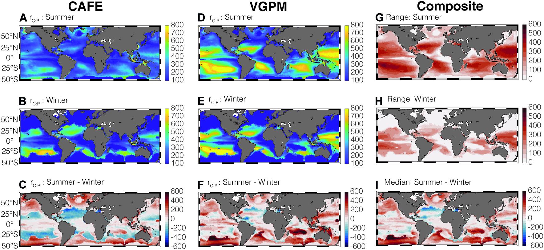
Figure 3. Global climatology of summer and winter average CAFE-informed rC:P (A–C) and VGPM-informed rC:P (D–F) in the surface mixed layer. rC:P is in molar units. Panels (G,H) show the maximum range in the four satellite-informed rC:P for summer and winter, respectively. Panel (I) shows the seasonal change in median rC:P.
Although the spatio-temporal pattern of rC:P is consistent across four satellite-informed cases for high-latitude regions and equatorial regions (Supplementary Figure 3), the range of the four satellite rC:P estimates is large in the subtropics (Figures 3G,H). This larger range reveals a relatively large uncertainty in rC:P in the subtropics. Here, we used range instead of arithmetic standard deviation as a measure of uncertainty because the ratios by their nature do not follow normal distributions (Isles, 2020) and the sample size is small (n = 4). We show the uncertainty of rC:P expressed in terms of geometric standard deviation from the mean in Supplementary Figure 5. Note that the spatial pattern of geometric standard deviation (Supplementary Figures 5A,B) is very similar to the spatial pattern of range (Figures 3G,H). Considering that the oligotrophic gyres tend to be P-limited throughout the year and the change in Chl:Cphyto is small, large uncertainties in μ are predominantly responsible for this uncertainty in rC:P in those regions of the global ocean. While the CAFE-informed rC:P shows a noticeable decrease during summer by ∼100–200 molar units (Figure 3C), VGPM-informed rC:P shows an increase during summer (Figure 3F).
In theory, rC:P should decrease as growth rate increases, and the fractional change in rC:P should be highest for low growth (Droop, 1974; Burmaster, 1979; Goldman et al., 1979; Morel, 1987). In other words, a small change in growth rate should lead to a large change in rC:P when the growth rate is low. Multiple culture experiments support this prediction, where phytoplankton growing at a high rate is both P-rich and has reduced stoichiometric flexibility (e.g., Hillebrand et al., 2013). If we assume P-limited growth condition and we replace growth rate with PO4 concentration, this pattern would also be true for PO4 vs. rC:P where phytoplankton growing under low P environment are frugal (high rC:P) and more stoichiometrically flexible (Galbraith and Martiny, 2015; Tanioka and Matsumoto, 2017, 2020a). As subtropical regions are strongly P limited and the growth is suppressed (Wu et al., 2000; Martiny et al., 2019), this reasoning can explain the elevated rC:P with large uncertainty and sensitivity.
Figure 4 illustrates how rC:P varies under varying growth rates and Chl:Cphyto in specific regions. Contour lines (isopleths) representing the theoretical values of rC:P are predicted by the Inomura phytoplankton stoichiometry model for different combinations of μ and Chl:Cphyto under the P limited scenario. In order to illustrate the regional variability, we superimposed monthly averaged, CAFE-informed rC:P in four oceanographic regions. These four regions are: (1) the high latitude bloom-forming North Atlantic Ocean (NAT: 25°W – 35°W, 45°N – 50°N), (2) the North Atlantic subtropical gyre (NASG: 25°W–70°W, 25°–35°N), (3) the South Pacific subtropical gyre (SPSG: 90°W–150°W, 15°S–40°S), and (4) the Equatorial upwelling region (EQU: 5°S – 5°N), following Westberry et al. (2016). The size of the symbol indicates the extent of P limitation. “P-replete” symbolizes <20% of grid boxes in the region are P-limited, “Moderate” symbolizes 20–80%, and “Deplete” >80% based on the seasonally varying SST. The numbers represent the month of the year.
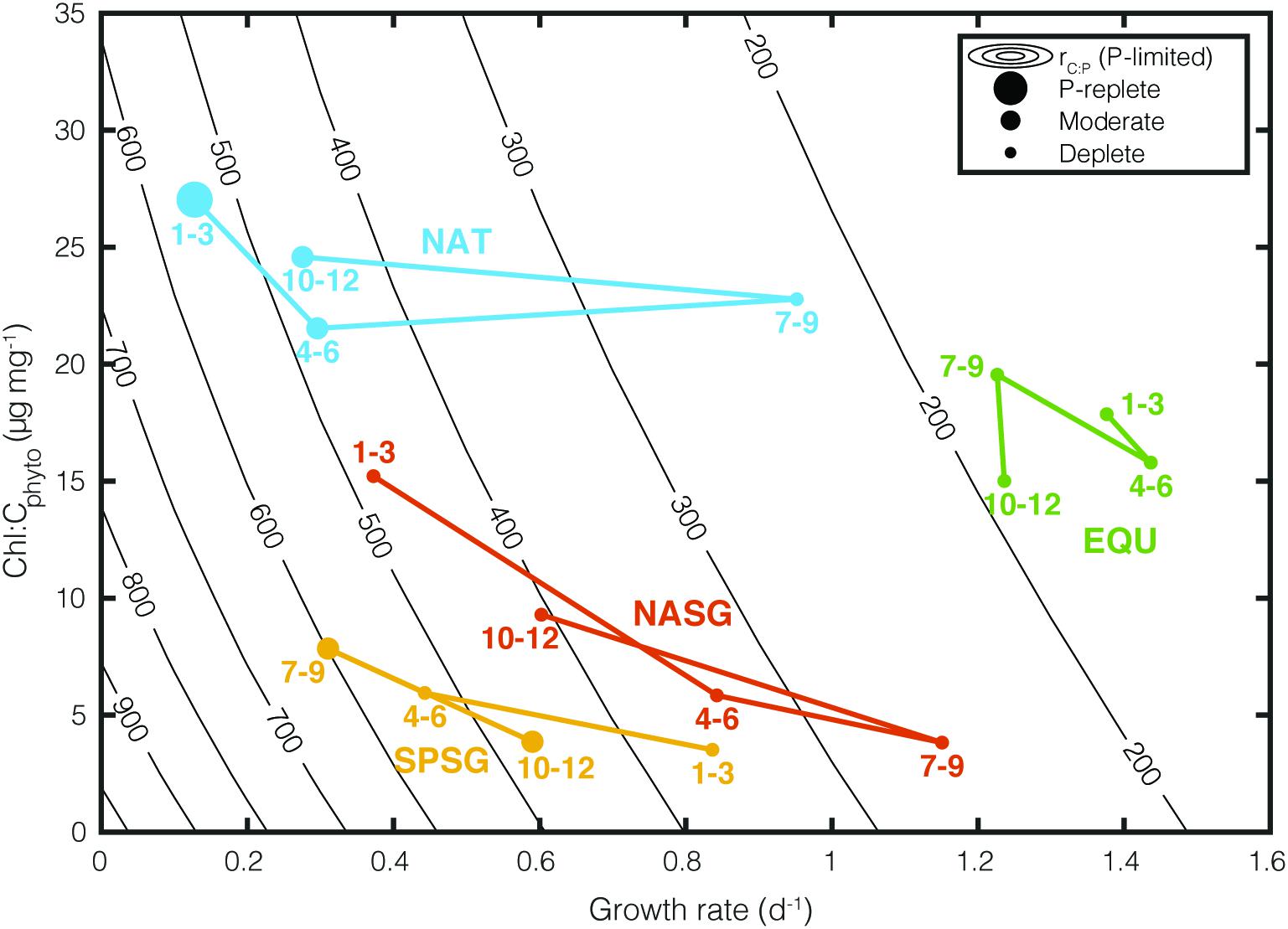
Figure 4. Influence of growth rate (μ) and Chl:Cphyto on rC:P under P limitation. Colored points represent seasonally averaged CAFE-informed Chl:Cphyto, μ, and rC:P for four oceanographic regions (NAT, North Atlantic Temperate; NASG, North Atlantic Subtropical Gyre; SPSG, South Pacific Subtropical Gyre; EQU, Equatorial Upwelling region. The marker size represents the degree of P limitation within the region (P-replete: <20% of the region is P-limited, Moderate: 20–80%, Deplete: >80%). The numbers next to the markers correspond to the months of the year. Contour lines show C:P calculated under varying μ and Chl:Cphyto with phytoplankton stoichiometry model under P-limited condition.
There are two key features in this plot. The first is that different oceanographic regions occupy a unique space. For example, North Atlantic (NAT) experiences large seasonal variability in growth rate, P limitation, and rC:P, while EQU experiences small seasonal changes. The second important feature is that the contours representing rC:P become increasingly close together as the growth rate decreases. This reiterates the fact that a small change in satellite-derived growth rate can lead to a large change in rC:P in chronically nutrient-deplete subtropical gyres (NASG and SPSG).
Light availability also affects rC:P as light modulates the cellular allocation between light-harvesting apparatus, biosynthetic apparatus, and energy storage reserves (Falkowski and LaRoche, 1991; Moreno and Martiny, 2018). The Inomura phytoplankton stoichiometry model predicts that increased light limitation increases cellular allocation toward photosynthetic proteins and decreases allocation toward C-rich biosynthetic proteins. Therefore, an increase in Chl:Cphyto (i.e., increased light limitation) will lead to a decrease in rC:P at a constant growth rate (Figure 4).
As expected, satellite-derived Chl:Cphyto shows maxima during winter months (January-March in Northern Hemisphere and July–September in Southern Hemisphere) due to decreased exposure to sunlight (Figure 4). As shown in previous modeling studies, the effect of light on rC:P is disproportionally large when the growth rate is low, and an increase in Chl:Cphyto can effectively reduce rC:P during winter months (Arteaga et al., 2014; Talmy et al., 2014). Compared to the growth rate, however, the effect of light limitation on rC:P is weak, as shown by the vertically steep contour lines in Figure 4. Indeed, a meta-analysis on published laboratory studies has shown that the effects of light on rC:P are significantly weaker than that of macronutrients and temperature (Tanioka and Matsumoto, 2020a).
Large-Scale Seasonal Variability in Bulk POC:POP
By combining the satellite-informed phytoplankton C:P and the community composition measured by Cphyto:POC, we can determine POC:POP of the bulk POM (Figure 5). Similar to rC:P, bulk POC:POP ratios are highest in the gyres compared to the equatorial upwelling and high-latitude regions. Globally, satellite POC:POP is higher during the summer compared to the winter. This seasonal trend can be explained by the higher Cphyto:POC during summer than winter (Supplementary Figure 2I). This makes intuitive sense because the phytoplankton biomass concentration is kept low in the mixed layer during winter months due to the deepening of MLD, strong light limitation, and zooplankton grazing (Behrenfeld and Boss, 2018). As C:P of P-limited phytoplankton is higher than C:P of non-algal organic matter, increase in Cphyto:POC during summer leads to an increase in POC:POP. The most noticeable increase is visible in the South Pacific Subtropic Gyre, where summertime POC:POP is higher than the winter value by ∼200 as Cphyto:POC increases by ∼50% during summer compared to winter. The range (uncertainty) in satellite-informed POC:POP (Figures 5G,H) is much smaller compared to that of phytoplankton C:P (Figures 3G,H), and all the four satellite-informed estimates agree on a general increase in POC:POP during summer compared to winter (Figure 5I and Supplementary Figure 4).
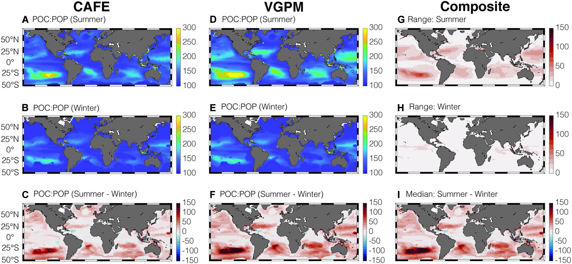
Figure 5. Global climatology of average summer and winter CAFE-informed POC:POP (A–C) and VGPM-informed POC:POP (D–F) in the surface mixed layer. Panels (G,H) show the range in satellite-informed POC:POP, for summer and winter, respectively. Panel (I) shows the seasonal change in median POC:POP.
Figure 6A illustrates how the bulk POC:POP is non-linearly related to the community composition (measured by Cphyto:POC) for a given change in rC:P. We observe from the satellite-derived data of Cphyto and POC that Cphyto:POC is, on average, ∼30% and rarely exceeds 50% of the total POC pool. The increase in POC:POP with respect to increase in rC:P reaches a plateau quickly when Cphyto:POC < 30%. In other words, the community dominance of non-algal POM over algal POM can effectively put a cap on the increase in bulk POC:POP, even when phytoplankton C:P is very high (e.g., NASG and SPSG). This top-down control on POC:POP due to community composition also explains the low uncertainty in the estimates of satellite-informed POC:POP despite the large uncertainty in satellite-informed rC:P.
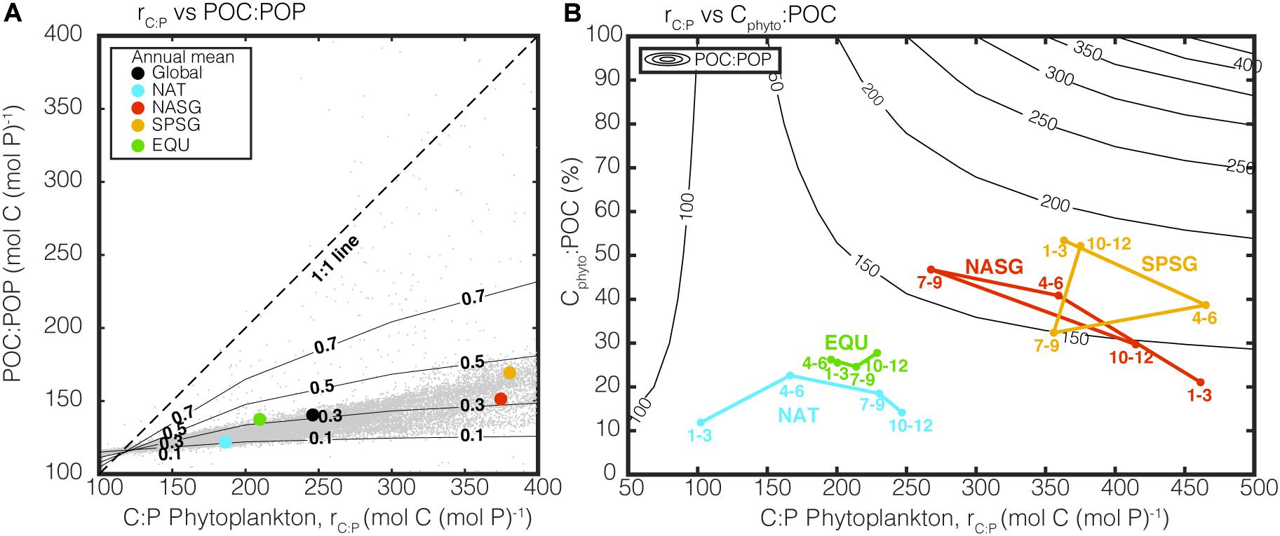
Figure 6. Two graphical representation of the influence of rC:P and Cphyto:POC on bulk POC:POP. In Panel (A), rC:P is plotted against POC:POP and contour lines show Cphyto:POC from 0 to 1. The colored dots are annual mean CAFE-informed rC:P and POC:POP from the selected regions, and the gray dots in the background are monthly predictions from each 1° by 1° grid point. In Panel (B), rC:P is plotted against Cphyto:POC and the contour lines show POC:POP. Colored points represent seasonally averaged POC:POP for four oceanographic regions, as in Figure 2. Both Panels (A,B) highlight the importance of top-down control on POC:POP by Cphyto:POC.
Figure 6B is an alternative way of illustrating this top-down control on bulk POC:POP by community composition. Contour lines representing POC:POP based on our simple two end-member algal/non-algal mixing model are widely separated when Cphyto:POC is low, indicating that POC:POP is relatively stable when Cphyto:POC is relatively low. On the other hand, when Cphyto:POC is high, contour lines become closer together, and bulk POC:POP quickly approaches rC:P. If we plot monthly averaged estimates of satellite-derived bulk POC:POP under different regions, two distinct clusters become apparent. Subtropical gyres (NASG and SPSG) are characterized by high rC:P and Cphyto:POC resulting in sizeable seasonal variability in bulk POC:POP. On the other hand, NAT and EQU experience a smaller seasonal change in POC:POP as the Cphyto:POC remains relatively constant around 15%. The take-home message from Figure 6 is that a community composition can exert a strong top-down control on POC:POP even when phytoplankton C:P is much higher than the Redfield ratio. Indeed, multiple studies emphasize this point, including recent studies on C:N (e.g., Talmy et al., 2016), N:P (e.g., Sharoni and Halevy, 2020), as well as the original study by Redfield et al. (1963).
Model-Data Comparison
To assess our model predictions, we first compare our seasonally resolved zonally averaged satellite POC:POP estimates with measurements of sampled POC:POP (Figure 7). Globally, both the satellite estimates and the in situ observations show higher POC:POP in summer (Figure 7A) than in winter (Figure 7B). This increase during summer is likely to be driven by a change in community composition, with an increased Cphyto:POC during summer. At high-latitudes, an increase in phytoplankton C:P also drives an increase in POC:POP during summer. Therefore, the combination of the change in community composition and phytoplankton C:P is responsible for the increased bulk POC:POP during summer.
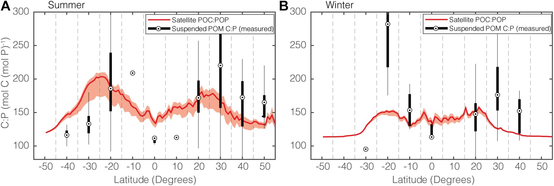
Figure 7. Comparisons of modeled and observed zonal POC:POP for (A) summer and (B) winter. The solid red curve shows the median POC:POP of the satellite-informed estimates, and shading shows the range. The black dot in the box and whisker plot show the median POC:POP, and the upper and lower edges of each box correspond to the upper and lower quantiles. The vertical tails correspond to a 95% confidence interval. When the sample size is 1, the sample variance could not be estimated, and only the dot representing unique POC:POP is shown (e.g., 10°N during Summer). Note that the satellite-informed POC:POP ratios are global latitudinal averages, whereas the measured POC:POP are averages of discrete data points.
Although it is promising that our predictions are mostly consistent with observations, there are two distinct regions where the satellite POC:POP and the observations do not agree. The first is the equatorial region during summer (Figure 7A), where satellite-informed POC:POP is around 150 but observed POC:POP is close to the Redfield ratio of 106. This discrepancy stems from the fact that our method likely overestimates the degree to which the equatorial regions are P-limited, which in turn leads to an overestimation of the phytoplankton C:P to as high as ∼200. In addition, our phytoplankton C:P model is tuned to data for Synechococcus. In reality, fast-growing opportunistic eukaryotic plankton such as diatoms and other eukaryotes with lower C:P are more predominant in the equatorial region (Arrigo, 2005; Martiny et al., 2013a; Kostadinov et al., 2016). The second region where we observed a noticeable difference between satellite estimates and in situ observation is around 20°S during winter (Figure 7B). Given the paucity of observations in this region, however, (n = 12 and 8 for summer and winter, respectively), it is challenging to determine the exact cause for the increase in POC:POP during the winter.
To further assess our model capability, we compare time-series data of suspended POC:POP in the top 100 m from BATS and HOT with satellite estimates in the seasonally mixed-layer depth from 2003 to 2010 (Figure 8). It is important to note that suspended POC:POP is a “point” value reflecting elemental composition at a particular location and at a particular time, whereas the satellite-informed POC:POP is a monthly and area-averaged value for a 3-by-3-pixel area around the BATS and HOT stations. We use the median satellite-informed phytoplankton C:P and POC:POP values from four satellite products (CAFE, VGPM, Eppley-VGPM, and CbPM) for comparison with the data. Here, we use the median rather than the mean as the measure of average C:P across satellite products because the ratios by their nature do not follow normal distributions (Isles, 2020).
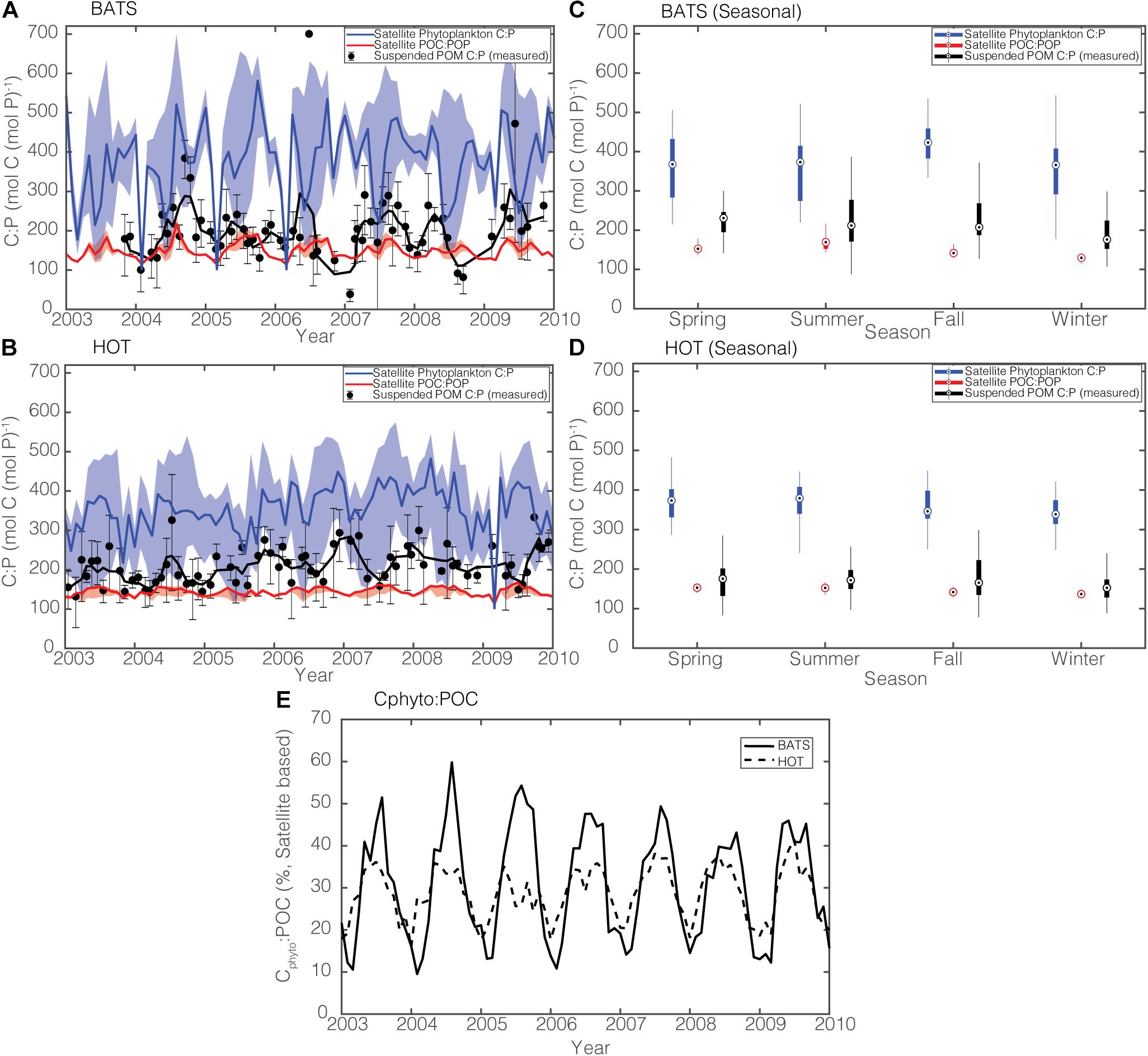
Figure 8. (A,B) Comparison of observed and modeled monthly C:P stoichiometry during 2003–2010 in the surface 100 m for BATS and HOT. Solid black lines are 3-month running means, and sample error bars are products of the geometric standard deviation and the geometric mean. Solid blue and red lines are median estimates for satellite-informed rC:P and POC:POP, respectively. The shadings show the range. (C,D) Box-whisker plot comparing the annual ratios of satellite-informed phytoplankton C:P (blue), satellite-informed POC:POP (red), and in situ POC:POP (black). Each season represents a 3-month average (Spring = April to June, Summer = July to September, Fall = October to December, Winter: January to March). (E) Satellite-derived Cphyto:POC at BATS (solid line) and at HOT (dotted line).
In general, measured POC:POP ratios lie between our satellite estimates of phytoplankton C:P and bulk POC:POP ratios at both BATS and HOT (Figures 8A,B). Measured POC:POP, on average, is closer to the satellite-informed POC:POP than to satellite-informed rC:P (Figures 8C,D). This makes intuitive sense because both satellite estimates (Figure 8E) and in situ observations (Casey et al., 2013) show that the biomass of picocyanobacteria (Prochlorococcus, Synechococcus) only contributes to <∼40% of the POC pool in the gyres. Qualitatively, our satellite estimates of bulk POC:POP seem to capture the general seasonal variability, with POC:POP being lowest in the winter and highest in the summer and the fall. Also, both the satellite-informed and the observed C:P are lowest in the late winter as a result of deep mixing and increased supply of nutrients, which cause phytoplankton C:P to decrease (Singh et al., 2015).
The amplitude of POC:POP variability is greater at BATS than at HOT, reflecting larger temporal variability in Cphyto:POC (Figure 8E). Phytoplankton carbon biomass can reach as high as 60% of the total POC pool at BATS during the growing season while the peak Cphyto:POC at HOT does not exceed ∼40%. This difference between the two sites may reflect the fact that the North Atlantic is a bottom-up ecosystem, while the North Pacific is a top-down ecosystem (Steele and Henderson, 1992; Siegel et al., 2016). Satellite-informed bulk POC:POP, however, underestimates the observed POC:POP by ∼50 on average at BATS (Figure 8C) and ∼20 at HOT (Figure 8D), and this may reflect the fact that non-algal organic matter has a higher ratio than Redfield of 117. Also, our satellite-informed estimate may not be fully capturing episodic temporal changes in C:P, for example, during the spring bloom when phytoplankton C:P is expected to increase rapidly (Polimene et al., 2015).
The satellite-informed estimates of phytoplankton C:P and POC:POP presented here are still preliminary and, therefore, should not be treated as accurate estimates. Nevertheless, even with this simple two-end-member mixing model approach, we can make a testable hypothesis regarding the underlying mechanisms causing the observed temporal change in suspended POC:POP. First, to model temporal shifts in POC:POP, we need to consider the contribution that non-algal organic matter makes to POM and the change in phytoplankton C:P. Our results indicate that phytoplankton C:P alone leads to a considerable overestimation of bulk POC:POP, regionally and globally. Second, our satellite-informed bulk POC:POP can capture the seasonal trend in POC:POP, which shows elevated values during summer compared to winter. We are optimistic that with more sophisticated parameter calibration of the phytoplankton stoichiometry model and non-algal C:P, it will be possible to predict the temporal variability of POC:POP accurately in future studies.
Caveats, Limitations, and Future Needs
Satellite estimates of phytoplankton and bulk C:P have considerable uncertainty in the subtropical gyres during summer. This mainly stems from the fact that satellite-derived growth-rate estimates are considerably different depending on which NPP product is used. In the future, we also need to conduct careful sensitivity analyses of how different satellite-based algorithms of Chl, Cphyto, and POC as well their depth-dependent changes would affect satellite-informed estimates of ecosystem stoichiometry. For example, a recent study suggests a substantial shift in POC:POP from the surface to DCM in the Indian Ocean during summer (Sahoo et al., 2020). It is inherently challenging to characterize C:P accurately in subtropics with phytoplankton stoichiometry models (Garcia et al., 2020) as phytoplankton turnover happens quickly on a time scale of days (Malone et al., 1993). For a complete understanding of the temporal variability of phytoplankton and bulk C:P, measurements of phytoplankton-specific C:P using high-throughput flow cytometry (Graff et al., 2015; Kirchman, 2016) or single-probe mass spectrometry (Sun et al., 2018) would be necessary. Linking metagenomics data with the phytoplankton stoichiometry model and remote sensing may also help improve C:P estimates in the subtropics (Garcia et al., 2020).
In this study, we used parameters for Synechococcus, a cosmopolitan phytoplankton species with a broad biogeographic distribution that extends from tropics to subpolar regions (Flombaum et al., 2013; Berube et al., 2018). This parameterization should be representative of another picocyanobacterium, Prochlorococcus. Together, Prochlorococcus and Synechococcus are responsible for roughly a quarter of the total ocean net primary productivity (Flombaum et al., 2013). Given that the current satellite-derived products cannot easily resolve size-partitioned phytoplankton physiologies such as growth rate and Chl:Cphyto, it seems reasonable to tune the phytoplankton stoichiometry model to these most common phytoplankton types. With new advances in satellite instrumentation, such as the development of reliable hyperspectral ocean color measurements (Werdell et al., 2018; Schollaert Uz et al., 2019), we may be able to better resolve the size-specific C:P of different phytoplankton functional types. This would enable us to fully capture the spatio-temporal variability of community phytoplankton C:P, particularly in nutrient-rich upwelling and coastal regions where nano- and micro-phytoplankton are more dominant than picophytoplankton (Kostadinov et al., 2016).
We inferred the P limitation of phytoplankton by comparing satellite-based SST and the previously compiled mask of nutrient depletion temperature. Although our method can provide a first-order pattern of P limitation, this method cannot resolve the degree to which phytoplankton are P-stressed. In other words, we cannot determine whether phosphate is the primary or secondary limiting nutrient for phytoplankton growth (Moore et al., 2013). Also, a recent study suggests that we cannot determine for sure that phytoplankton is P-limited even when the observed phosphate concentration is below the detection limit (Martiny et al., 2019). Accurate determination of nutrient concentration from space is inherently challenging (Goes et al., 2000; Steinhoff et al., 2010; Arteaga et al., 2015), and this is one of the major bottlenecks for accurately probing phytoplankton nutrient limitation from space. Although there are no standard protocols or algorithms currently available, we may be able to accurately retrieve surface nutrient concentrations by using advanced statistical and machine learning techniques applied to satellite-retrieved sea surface salinity, temperature, and remote-sensing reflectance (e.g., Wang et al., 2018).
A fundamental assumption made when predicting bulk POC:POP is that C:P of non-algal organic matter is constant with a Redfield Ratio of 117. There is a consensus from previous marine and freshwater studies that C:P of heterotrophs is generally lower and more homeostatic (relatively constant) than that of phytoplankton (Elser and Urabe, 1999; Persson et al., 2010). The bulk POM, however, can be modified due to decomposition (Schneider et al., 2003), viral shunt (Jover et al., 2014), preferential remineralization (Shaffer et al., 1999), as well as the interplay between the dissolved and particulate pools. Measuring the elemental composition of separate constituents of organic matter should better help us constrain the most appropriate end-member C:P for non-algal organic matter. Alternatively, we can mechanistically predict C:P of bulk POM by coupling the phytoplankton stoichiometry model with models of prey-predator interaction and decomposition (e.g., Anderson et al., 2005; Butenschön et al., 2016; Tanioka and Matsumoto, 2018).
Conclusion
We showed that it is possible to determine spatially and temporally coherent patterns of the C:P ratios of a single class of marine phytoplankton and bulk POM using only remotely sensed information. In principle, the same method can be extended to the C:N ratio, which together with the C:P ratio can yield the N:P ratio. The results shown here should not be treated as accurate estimates of upper-ocean C:P but rather as a feasibility study that can benefit from more accurate remotely sensed estimates of growth rate and from a better understanding of the links between growth rate and stoichiometry for different size classes of marine phytoplankton. The number of measurements of the C:P ratio of individual POM components (i.e., algal and non-algal components) is currently insufficient to validate our estimates. However, our main conclusion highlighting the importance of community composition in controlling bulk POC:POP does not depend on the accuracy of stoichiometry estimates. This conclusion has important implications for estimating carbon and phosphorus fluxes to the deep ocean and for the trophic transfer to higher organisms. Indeed, if the POC:POP of exported POM is controlled by community composition rather than phytoplankton C:P, we would not expect large “stoichiometric buffering” of carbon export under climate-change scenarios as proposed by previous studies (Teng et al., 2014; Galbraith and Martiny, 2015; Tanioka and Matsumoto, 2017; Matsumoto et al., 2020a). However, the effects of change in phytoplankton C:P will become more critical for carbon export if the total % of phytoplankton in organic matter increases, or if the C:P of the non-algal component increases. We hope the questions raised here will foster collaborative work combining satellite remote sensing, field sampling, and numerical modeling specialists to improve our ability to predict organic-matter dynamics and reduce uncertainties in our projections of the future carbon cycle.
Data Availability Statement
The datasets presented in this study can be found in online repositories. The names of the repository/repositories and accession number(s) can be found below: https://doi.org/10.5281/zenodo.4136353.
Author Contributions
TT, CF, and KM designed the study. TT gathered and analyzed data. All the authors wrote the manuscript.
Funding
This research was supported by US National Science Foundation (OCE-1827948, KM). The funding supports the project “A power law model of dynamic marine phytoplankton stoichiometry,” aimed at developing a new approach to representing stoichiometric diversity in ocean models and by quantifying the global impacts of that diversity under different climate conditions.
Conflict of Interest
The authors declare that the research was conducted in the absence of any commercial or financial relationships that could be construed as a potential conflict of interest.
Supplementary Material
The Supplementary Material for this article can be found online at: https://www.frontiersin.org/articles/10.3389/fmars.2020.604893/full#supplementary-material
Footnotes
- ^ http://sites.science.oregonstate.edu/ocean.productivity/index.php (last access: June 22, 2020)
- ^ http://oceancolor.gsfc.nasa.gov (last access: June 22, 2020)
References
Anderson, L. A., and Sarmiento, J. L. (1994). Redfield ratios of remineralization determined by nutrient data analysis. Glob. Biogeochem. Cycl. 8, 65–80. doi: 10.1029/93GB03318
Anderson, T. R., Hessen, D. O., Elser, J. J., and Urabe, J. (2005). Metabolic Stoichiometry and the Fate of Excess Carbon and Nutrients in Consumers. Am. Nat. 165, 1–15. doi: 10.1086/426598
Arora, V. K., Katavouta, A., Williams, R. G., Jones, C. D., Brovkin, V., Friedlingstein, P., et al. (2020). Carbon–concentration and carbon–climate feedbacks in CMIP6 models and their comparison to CMIP5 models. Biogeosciences 17, 4173–4222. doi: 10.5194/bg-17-4173-2020
Arrigo, K. R. (2005). Marine microorganisms and global nutrient cycles. Nature 437, 349–355. doi: 10.1038/nature04159
Arteaga, L., Pahlow, M., and Oschlies, A. (2014). Global patterns of phytoplankton nutrient and light colimitation inferred from an optimality-based model. Glob. Biogeochem. Cycl. 28, 648–661. doi: 10.1002/2013GB004668
Arteaga, L., Pahlow, M., and Oschlies, A. (2015). Global monthly sea surface nitrate fields estimated from remotely sensed sea surface temperature, chlorophyll, and modeled mixed layer depth. Geophys. Res. Lett. 42, 1130–1138. doi: 10.1002/2014GL062937
Arteaga, L., Pahlow, M., and Oschlies, A. (2016). Modelled Chl:C ratio and derived estimates of phytoplankton carbon biomass and its contribution to total particulate organic carbon in the global surface ocean. Glob. Biogeochem. Cycl. 30, 1791–1810. doi: 10.1002/2016GB005458
Behrenfeld, M. J., Boss, E., Siegel, D. A., and Shea, D. M. (2005). Carbon-based ocean productivity and phytoplankton physiology from space. Glob. Biogeochem. Cycl. 19, 1–14. doi: 10.1029/2004GB002299
Behrenfeld, M. J., and Boss, E. S. (2018). Student’s tutorial on bloom hypotheses in the context of phytoplankton annual cycles. Glob. Chang. Biol. 24, 55–77. doi: 10.1111/gcb.13858
Behrenfeld, M. J., and Falkowski, P. G. (1997). Photosynthetic rates derived from satellite-based chlorophyll concentration. Limnol. Oceanogr. 42, 1–20. doi: 10.4319/lo.1997.42.1.0001
Bellacicco, M., Volpe, G., Briggs, N., Brando, V., Pitarch, J., Landolfi, A., et al. (2018). Global distribution of non-algal particles from ocean color data and implications for phytoplankton biomass detection. Geophys. Res. Lett. 45, 7672–7682. doi: 10.1029/2018GL078185
Berube, P. M., Biller, S. J., Hackl, T., Hogle, S. L., Satinsky, B. M., Becker, J. W., et al. (2018). Data descriptor: single cell genomes of Prochlorococcus. Synechococcus, and sympatric microbes from diverse marine environments. Sci. Data 5, 1–11. doi: 10.1038/sdata.2018.154
Bisson, K. M., Siegel, D. A., DeVries, T., Cael, B. B., and Buesseler, K. O. (2018). How data set characteristics influence ocean carbon export models. Global Biogeochem. Cycles 32, 1312–1328. doi: 10.1029/2018GB005934
Bopp, L., Resplandy, L., Orr, J. C., Doney, S. C., Dunne, J. P., Gehlen, M., et al. (2013). Multiple stressors of ocean ecosystems in the 21st century: projections with CMIP5 models. Biogeosciences 10, 6225–6245. doi: 10.5194/bg-10-6225-2013
Burmaster, D. E. (1979). The continuous culture of phytoplankton: mathematical equivalence among three steady-state models. Am. Nat. 113:123. doi: 10.1086/283368
Butenschön, M., Clark, J., Aldridge, J. N., Icarus Allen, J., Artioli, Y., Blackford, J., et al. (2016). ERSEM 15.06: a generic model for marine biogeochemistry and the ecosystem dynamics of the lower trophic levels. Geosci. Model Dev. 9, 1293–1339. doi: 10.5194/gmd-9-1293-2016
Casey, J. R., Aucan, J. P., Goldberg, S. R., and Lomas, M. W. (2013). Changes in partitioning of carbon amongst photosynthetic pico- and nano-plankton groups in the Sargasso Sea in response to changes in the North Atlantic Oscillation. Deep. Res. Part II Top. Stud. Oceanogr. 93, 58–70. doi: 10.1016/j.dsr2.2013.02.002
Copin-Montegut, C., and Copin-Montegut, G. (1983). Stoichiometry of carbon, nitrogen, and phosphorus in marine particulate matter. Deep Sea Res. Part A. Oceanogr. Res. Pap. 30, 31–46. doi: 10.1016/0198-0149(83)90031-6
Cullen, J. J. (1982). The deep chlorophyll maximum: comparing vertical profiles of chlorophyll a. Can. J. Fish. Aquat. Sci. 39, 791–803. doi: 10.1139/f82-108
Dierssen, H. M. (2010). Perspectives on empirical approaches for ocean color remote sensing of chlorophyll in a changing climate. Proc. Natl. Acad. Sci. U.S.A. 107, 17073–17078. doi: 10.1073/pnas.0913800107
Droop, M. R. (1974). The nutrient status of algal cells in continuous culture. J. Mar. Biol. Assoc. U.K. 54, 825–855. doi: 10.1017/S002531540005760X
Durand, M. D., Olson, R. J., and Chisholm, S. W. (2001). Phytoplankton population dynamics at the bermuda atlantic time-series station in the sargasso sea. Deep. Res. Part II Top. Stud. Oceanogr. 48, 1983–2003. doi: 10.1016/S0967-0645(00)00166-1
Dutkiewicz, S., Hickman, A. E., Jahn, O., Henson, S., Beaulieu, C., and Monier, E. (2019). Ocean colour signature of climate change. Nat. Commun. 10:578. doi: 10.1038/s41467-019-08457-x
Elser, J. J., and Urabe, J. (1999). The stoichiometry of consumer-driven nutrient recycling: theory, observations, and consequences. Ecology 80, 735–751. doi: 10.2307/177013
Eppley, R. W., Chavez, F. P., and Barber, R. T. (1992). Standing stocks of particulate carbon and nitrogen in the equatorial Pacific at 150°W. J. Geophys. Res. 97:655. doi: 10.1029/91JC01386
Evers-King, H., Martinez-Vicente, V., Brewin, R. J. W., Dall’Olmo, G., Hickman, A. E., Jackson, T., et al. (2017). Validation and intercomparison of ocean color algorithms for estimating particulate organic carbon in the oceans. Front. Mar. Sci. 4:251. doi: 10.3389/fmars.2017.00251
Fagan, A. J., Moreno, A. R., and Martiny, A. C. (2019). Role of ENSO conditions on particulate organic matter concentrations and elemental ratios in the southern california bight. Front. Mar. Sci. 6:386. doi: 10.3389/fmars.2019.00386
Falkowski, P. G., Dubinsky, Z., and Wyman, K. (1985). Growth–irradiance relationships in phytoplankton. Limnol. Oceanogr. 30, 311–321. doi: 10.4319/lo.1985.30.2.0311
Falkowski, P. G., and LaRoche, J. (1991). Acclimation to Spectral Irradiance in Algae. J. Phycol. 27, 8–14. doi: 10.1111/j.0022-3646.1991.00008.x
Finkel, Z. V., Follows, M. J., and Irwin, A. J. (2016). Size-scaling of macromolecules and chemical energy content in the eukaryotic microalgae. J. Plankton Res. 38, 1151–1162. doi: 10.1093/plankt/fbw057
Flombaum, P., Gallegos, J. L., Gordillo, R. A., Rincón, J., Zabala, L. L., Jiao, N., et al. (2013). Present and future global distributions of the marine Cyanobacteria Prochlorococcus and Synechococcus. Proc. Natl. Acad. Sci. U.S.A. 110, 9824–9829. doi: 10.1073/pnas.1307701110
Fumenia, A., Petrenko, A., Loisel, H., Djaoudi, K., deVerneil, A., and Moutin, T. (2020). Optical proxy for particulate organic nitrogen from Bio Argo floats. Opt. Express 28, 21391–21406. doi: 10.1364/oe.395648
Galbraith, E. D., and Martiny, A. C. (2015). A simple nutrient-dependence mechanism for predicting the stoichiometry of marine ecosystems. Proc. Natl. Acad. Sci. U.S.A. 112, 8199–8204. doi: 10.1073/pnas.1423917112
Garcia, C. A., Baer, S. E., Garcia, N. S., Rauschenberg, S., Twining, B. S., Lomas, M. W., et al. (2018). Nutrient supply controls particulate elemental concentrations and ratios in the low latitude eastern Indian Ocean. Nat. Commun. 9:4868. doi: 10.1038/s41467-018-06892-w
Garcia, C. A., Hagstrom, G. I., Larkin, A. A., Ustick, L. J., Levin, S. A., Lomas, M. W., et al. (2020). Linking regional shifts in microbial genome adaptation with surface ocean biogeochemistry. Philos. Trans. R. Soc. B Biol. Sci. 375:20190254. doi: 10.1098/rstb.2019.0254
Geider, R. J. (1987). Light and temperature dependence of the carbon to chlorophyll a ratio in microalgae and cyanobacteria: implications for physiology and growth of phytoplankton. New Phytol. 106, 1–34. doi: 10.1111/j.1469-8137.1987.tb04788.x
Goes, J. I., Saino, T., Oaku, H., Ishizaka, J., Wong, C. S., and Nojiri, Y. (2000). Basin scale estimates of Sea Surface nitrate and new production from remotely sensed sea surface temperature and chlorophyll. Geophys. Res. Lett. 27, 1263–1266. doi: 10.1029/1999GL002353
Goldman, J. C., McCarthy, J. J., and Peavey, D. G. (1979). Growth rate influence on the chemical composition of phytoplankton in oceanic waters. Nature 279, 210–215. doi: 10.1038/279210a0
Graff, J. R., Westberry, T. K., Milligan, A. J., Brown, M. B., Dall’Olmo, G., van Dongen-Vogels, V., et al. (2015). Analytical phytoplankton carbon measurements spanning diverse ecosystems. Deep. Res. Part I Oceanogr. Res. Pap. 102, 16–25. doi: 10.1016/j.dsr.2015.04.006
Gundersen, K., Heldal, M., Norland, S., Purdie, D. A., and Knap, A. H. (2002). Elemental C. N, and P cell content of individual bacteria collected at the Bermuda Atlantic Time-series Study (BATS) site. Limnol. Oceanogr. 47, 1525–1530. doi: 10.4319/lo.2002.47.5.1525
Gundersen, K., Orcutt, K. M., Purdie, D. A., Michaels, A. F., and Knap, A. H. (2001). Particulate organic carbon mass distribution at the Bermuda Atlantic Time-series Study (BATS) site. Deep Sea Res. Part II Top. Stud. Oceanogr. 48, 1697–1718. doi: 10.1016/S0967-0645(00)00156-9
Healey, F. P. (1985). Interacting effects of light and nutrient limitation on the growth rate of Synechococcus linearis (cyanophyceae). J. Phycol. 21, 134–146. doi: 10.1111/j.0022-3646.1985.00134.x
Hebel, D. V., and Karl, D. M. (2001). Seasonal, interannual and decadal variations in particulate matter concentrations and composition in the subtropical North Pacific Ocean. Deep Sea Res. Part II Top. Stud. Oceanogr. 48, 1669–1695. doi: 10.1016/S0967-0645(00)00155-7
Hillebrand, H., Steinert, G., Boersma, M., Malzahn, A., Meunier, C. L., Plum, C., et al. (2013). Goldman revisited: faster-growing phytoplankton has lower N?: P and lower stoichiometric flexibility. Limnol. Oceanogr. 58, 2076–2088. doi: 10.4319/lo.2013.58.6.2076
Inomura, K., Omta, A. W., Talmy, D., Bragg, J., Deutsch, C., and Follows, M. J. (2020). A Mechanistic Model of Macromolecular Allocation, Elemental Stoichiometry, and Growth Rate in Phytoplankton. Front. Microbiol. 11:86. doi: 10.3389/fmicb.2020.00086
Isles, P. D. F. (2020). The misuse of ratios in ecological stoichiometry. Ecology 0, 1–7. doi: 10.1002/ecy.3153
Jamet, C., Ibrahim, A., Ahmad, Z., Angelini, F., Babin, M., Behrenfeld, M. J., et al. (2019). Going Beyond Standard Ocean Color Observations: lidar and Polarimetry. Front. Mar. Sci. 6:251. doi: 10.3389/fmars.2019.00251
Jover, L. F., Effler, T. C., Buchan, A., Wilhelm, S. W., and Weitz, J. S. (2014). The elemental composition of virus particles: implications for marine biogeochemical cycles. Nat. Rev. Microbiol. 12, 519–528. doi: 10.1038/nrmicro3289
Kamykowski, D., and Zentara, S. J. (1986). Predicting plant nutrient concentrations from temperature and sigma-t in the upper kilometer of the world ocean. Deep Sea Res. Part A, Oceanogr. Res. Pap. 33, 89–105. doi: 10.1016/0198-0149(86)90109-3
Kamykowski, D., Zentara, S.-J., Morrison, J. M., and Switzer, A. C. (2002). Dynamic global patterns of nitrate, phosphate, silicate, and iron availability and phytoplankton community composition from remote sensing data. Glob. Biogeochem. Cycl. 16, 25–29. doi: 10.1029/2001GB001640
Kara, A. B., Rochford, P. A., and Hurlburt, H. E. (2003). Mixed layer depth variability over the global ocean. J. Geophys. Res. 108:3079. doi: 10.1029/2000JC000736
Karl, D. M., Björkman, K. M., Dore, J. E., Fujieki, L., Hebel, D. V., Houlihan, T., et al. (2001). Ecological nitrogen-to-phosphorus stoichiometry at station ALOHA. Deep Sea Res. Part II Top. Stud. Oceanogr 48, 1529–1566. doi: 10.1016/S0967-0645(00)00152-1
Kilham, P., and Hecky, R. E. (1988). Comparative ecology of marine and freshwater phytoplankton. Limnol. Oceanogr. 33, 776–795. doi: 10.4319/lo.1988.33.4part2.0776
Kirchman, D. L. (2016). Growth rates of microbes in the oceans. Ann. Rev. Mar. Sci. 8, 285–309. doi: 10.1146/annurev-marine-122414-033938
Kostadinov, T. S., Milutinovi, S., Marinov, I., and Cabré, A. (2016). Carbon-based phytoplankton size classes retrieved via ocean color estimates of the particle size distribution. Ocean Sci. 12, 561–575. doi: 10.5194/os-12-561-2016
Laws, E. A. (2013). Evaluation of in situ phytoplankton growth rates: a synthesis of data from varied approaches. Ann. Rev. Mar. Sci. 5, 247–268. doi: 10.1146/annurev-marine-121211-172258
Laws, E. A., and Bannister, T. T. (1980). Nutrient- and light-limited growth of Thalassiosira fluviatilis in continuous culture, with implications for phytoplankton growth in the ocean. Limnol. Oceanogr. 25, 457–473. doi: 10.4319/lo.1980.25.3.0457
Lee, S., and Fuhrman, J. A. (1987). Relationships between biovolume and biomass of naturally derived marine bacterioplankton. Appl. Environ. Microbiol. 53, 1298–1303. doi: 10.1128/aem.53.6.1298-1303.1987
Levitus, S. (1982). Climatological Atlas of the World Ocean. Washington, DC: National Oceanic and Atmospheric Administration.
Liénart, C., Savoye, N., David, V., Ramond, P., Rodriguez Tress, P., Hanquiez, V., et al. (2018). Dynamics of particulate organic matter composition in coastal systems: forcing of spatio-temporal variability at multi-systems scale. Prog. Oceanogr. 162, 271–289. doi: 10.1016/j.pocean.2018.02.026
Loisel, H., Lubac, B., Dessailly, D., Duforet-Gaurier, L., and Vantrepotte, V. (2010). Effect of inherent optical properties variability on the chlorophyll retrieval from ocean color remote sensing: an in situ approach. Opt. Express 18:20949. doi: 10.1364/oe.18.020949
MacIntyre, H. L., Kana, T. M., Anning, T., and Geider, R. J. (2002). Photoacclimation of photosynthesis irradiance response curves and photosynthetic pigments in microalgae and cyanobacteria. J. Phycol. 38, 17–38. doi: 10.1046/j.1529-8817.2002.00094.x
Malone, T. C., Pike, S. E., and Conley, D. J. (1993). Transient variations in phytoplankton productivity at the JGOFS Bermuda time series station. Deep Sea Res. Part I Oceanogr. Res. Pap. 40, 903–924. doi: 10.1016/0967-0637(93)90080-M
Martínez-Vicente, V., Evers-King, H., Roy, S., Kostadinov, T. S., Tarran, G. A., Graff, J. R., et al. (2017). Intercomparison of ocean color algorithms for picophytoplankton carbon in the ocean. Front. Mar. Sci. 4:378. doi: 10.3389/fmars.2017.00378
Martiny, A. C., Lomas, M. W., Fu, W., Boyd, P. W., Chen, Y. L., Cutter, G. A., et al. (2019). Biogeochemical controls of surface ocean phosphate. Sci. Adv. 5:eaax0341. doi: 10.1126/sciadv.aax0341
Martiny, A. C., Pham, C. T. A., Primeau, F. W., Vrugt, J. A., Moore, J. K., Levin, S. A., et al. (2013a). Strong latitudinal patterns in the elemental ratios of marine plankton and organic matter. Nat. Geosci. 6, 279–283. doi: 10.1038/ngeo1757
Martiny, A. C., Talarmin, A., Mouginot, C., Lee, J. A., Huang, J. S., Gellene, A. G., et al. (2016). Biogeochemical interactions control a temporal succession in the elemental composition of marine communities. Limnol. Oceanogr. 61, 531–542. doi: 10.1002/lno.10233
Martiny, A. C., Vrugt, J. A., and Lomas, M. W. (2014). Concentrations and ratios of particulate organic carbon, nitrogen, and phosphorus in the global ocean. Sci. Data 1:140048. doi: 10.1038/sdata.2014.48
Martiny, A. C., Vrugt, J. A., Primeau, F. W., and Lomas, M. W. (2013b). Regional variation in the particulate organic carbon to nitrogen ratio in the surface ocean. Glob. Biogeochem. Cycles 27, 723–731. doi: 10.1002/gbc.20061
Matsumoto, K., Rickaby, R., and Tanioka, T. (2020a). Carbon export buffering and CO2 drawdown by Flexible Phytoplankton C:N:P under glacial conditions. Paleoceanogr. Paleoclimatol. 35:e2019A003823. doi: 10.1029/2019PA003823
Matsumoto, K., Tanioka, T., and Rickaby, R. (2020b). Linkages between dynamic phytoplankton C:N:P and the ocean carbon cycle under climate change. Oceanography 33, 44–52. doi: 10.5670/oceanog.2020.203
Moore, C. M., Mills, M. M., Arrigo, K. R., Berman-Frank, I., Bopp, L., Boyd, P. W., et al. (2013). Processes and patterns of oceanic nutrient limitation. Nat. Geosci. 6, 701–710. doi: 10.1038/ngeo1765
Morel, A., and Gentili, B. (2009). A simple band ratio technique to quantify the colored dissolved and detrital organic material from ocean color remotely sensed data. Remote Sens. Environ. 113, 998–1011. doi: 10.1016/j.rse.2009.01.008
Morel, F. M. M. (1987). Kinetics of nutrient uptake and growth in phytoplankton. J. Phycol. 23, 137–150. doi: 10.1111/j.0022-3646.1987.00137.x
Moreno, A. R., and Martiny, A. C. (2018). Ecological Stoichiometry of Ocean Plankton. Ann. Rev. Mar. Sci. 10, 43–69. doi: 10.1146/annurev-marine-121916-063126
Ödalen, M., Nycander, J., Ridgwell, A., Oliver, K. I. C., Peterson, C. D., and Nilsson, J. (2020). Variable C/P composition of organic production and its effect on ocean carbon storage in glacial-like model simulations. Biogeosciences 17, 2219–2244. doi: 10.5194/bg-17-2219-2020
Pahlow, M., Dietze, H., and Oschlies, A. (2013). Optimality-based model of phytoplankton growth and diazotrophy. Mar. Ecol. Prog. Ser. 489, 1–16. doi: 10.3354/meps10449
Persson, J., Fink, P., Goto, A., Hood, J. M., Jonas, J., and Kato, S. (2010). To be or not to be what you eat: regulation of stoichiometric homeostasis among autotrophs and heterotrophs. Oikos 119, 741–751. doi: 10.1111/j.1600-0706.2009.18545.x
Polimene, L., Mitra, A., Sailley, S. F., Ciavatta, S., Widdicombe, C. E., Atkinson, A., et al. (2015). Decrease in diatom palatability contributes to bloom formation in the Western English Channel. Prog. Oceanogr. 137, 484–497. doi: 10.1016/j.pocean.2015.04.026
Rasse, R., Dall’Olmo, G., Graff, J., Westberry, T. K., van Dongen-Vogels, V., and Behrenfeld, M. J. (2017). Evaluating optical proxies of particulate organic carbon across the surface atlantic ocean. Front. Mar. Sci. 4:367. doi: 10.3389/fmars.2017.00367
Redfield, A. C. (1934). On the proportions of organic derivatives in sea water and their relation to the composition of plankton. Univ. Press Liverpool. James Johnstone Meml. 1934, 177–192.
Redfield, A. C., Ketchum, B. H., and Richards, F. A. (1963). “The influence of organisms on the composition of Seawater,” in The Composition of Seawater: Comparative and Descriptive Oceanography. The Sea: Ideas and Observations on Progress in the Study of the Seas, ed. M. N. Hill (New York, NY: Interscience Publishers), 26–77.
Roy, S. (2018). Distributions of phytoplankton carbohydrate, protein and lipid in the world oceans from satellite ocean colour. ISME J. 12, 1457–1472. doi: 10.1038/s41396-018-0054-8
Sahoo, D., Saxena, H., Tripathi, N., Atif Khan, M., Rahman, A., Kumar, S., et al. (2020). Non-Redfieldian C:N:P ratio in the inorganic and organic pools of the Bay of Bengal during the summer monsoon. Mar. Ecol. Prog. Ser. 653, 41–45. doi: 10.3354/meps13498
Schneider, B., Schlitzer, R., Fischer, G., and Nöthig, E.-M. (2003). Depth-dependent elemental compositions of particulate organic matter (POM) in the ocean. Glob. Biogeochem. Cycles 17:1032. doi: 10.1029/2002GB001871
Schollaert Uz, S., Kim, G. E., Mannino, A., Werdell, P. J., and Tzortziou, M. (2019). Developing a community of practice for applied uses of future PACE data to address marine food security challenges. Front. Earth Sci. 7:283. doi: 10.3389/feart.2019.00283
Shaffer, G., Bendtsen, J., and Ulloa, O. (1999). Fractionation during remineralization of organic matter in the ocean. Deep. Res. Part I Oceanogr. Res. Pap. 46, 185–204. doi: 10.1016/S0967-0637(98)00061-2
Sharoni, S., and Halevy, I. (2020). Nutrient ratios in marine particulate organic matter are predicted by the population structure of well-adapted phytoplankton. Sci. Adv. 6:eaaw9371. doi: 10.1126/sciadv.aaw9371
Siegel, D. A., Buesseler, K. O., Behrenfeld, M. J., Benitez-Nelson, C., Boss, E., Brzezinski, M. A., et al. (2016). Prediction of the export and fate of global ocean net primary production: the EXPORTS Science Plan. Front. Mar. Sci 3:22. doi: 10.3389/fmars.2016.00022
Siegel, D. A., Maritorena, S., Nelson, N. B., Behrenfeld, M. J., and McClain, C. R. (2005). Colored dissolved organic matter and its influence on the satellite-based characterization of the ocean biosphere. Geophys. Res. Lett. 32, 1–4. doi: 10.1029/2005GL024310
Silsbe, G. M., Behrenfeld, M. J., Halsey, K. H., Milligan, A. J., and Westberry, T. K. (2016). The CAFE model: a net production model for global ocean phytoplankton. Glob. Biogeochem. Cycles 30, 1756–1777. doi: 10.1002/2016GB005521
Singh, A., Baer, S. E., Riebesell, U., Martiny, A. C., and Lomas, M. W. (2015). C : N : P stoichiometry at the Bermuda Atlantic Time-series Study station in the North Atlantic Ocean. Biogeosciences 12, 6389–6403. doi: 10.5194/bg-12-6389-2015
Steele, J. H., and Henderson, E. W. (1992). The role of predation in plankton models. J. Plankton Res. 14, 157–172. doi: 10.1093/plankt/14.1.157
Steinhoff, T., Friedrich, T., Hartman, S. E., Oschlies, A., Wallace, D. W. R., and Körtzinger, A. (2010). Estimating mixed layer nitrate in the North Atlantic Ocean. Biogeosciences 7, 795–807. doi: 10.5194/bg-7-795-2010
Sterner, R. W., Andersen, T., Elser, J. J., Hessen, D. O., Hood, J. M., McCauley, E., et al. (2008). Scale-dependent carbon:nitrogen:phosphorus seston stoichiometry in marine and freshwaters. Limnol. Oceanogr. 53, 1169–1180. doi: 10.4319/lo.2008.53.3.1169
Sterner, R. W., and Elser, J. J. (2002). Ecological Stoichiometry: The Biology of Elements From Molecules to the Biosphere. Princeton, NJ: Princeton University Press.
Stramski, D., Reynolds, R. A., Babin, M., Kaczmarek, S., Lewis, M. R., Röttgers, R., et al. (2008). Relationships between the surface concentration of particulate organic carbon and optical properties in the eastern South Pacific and eastern Atlantic Oceans. Biogeosciences 5, 171–201. doi: 10.5194/bg-5-171-2008
Sun, M., Yang, Z., and Wawrik, B. (2018). Metabolomic fingerprints of individual algal cells using the single-probe mass spectrometry technique. Front. Plant Sci. 9:571. doi: 10.3389/fpls.2018.00571
Talarmin, A., Lomas, M. W., Bozec, Y., Savoye, N., Frigstad, H., Karl, D. M., et al. (2016). Seasonal and long-term changes in elemental concentrations and ratios of marine particulate organic matter. Glob. Biogeochem. Cycles 30, 1699–1711. doi: 10.1002/2016GB005409
Talmy, D., Blackford, J., Hardman-Mountford, N. J., Polimene, L., Follows, M. J., and Geider, R. J. (2014). Flexible C : N ratio enhances metabolism of large phytoplankton when resource supply is intermittent. Biogeosciences 11, 4881–4895. doi: 10.5194/bg-11-4881-2014
Talmy, D., Martiny, A. C., Hill, C., Hickman, A. E., and Follows, M. J. (2016). Microzooplankton regulation of surface ocean POC:PON ratios. Glob. Biogeochem. Cycles 30, 311–332. doi: 10.1002/2015GB005273
Tanioka, T., and Matsumoto, K. (2017). Buffering of ocean export production by flexible elemental stoichiometry of particulate organic matter. Glob. Biogeochem. Cycles 31, 1528–1542. doi: 10.1002/2017GB005670
Tanioka, T., and Matsumoto, K. (2018). Effects of incorporating age-specific traits of zooplankton into a marine ecosystem model. Ecol. Modell. 368, 257–264. doi: 10.1016/j.ecolmodel.2017.11.024
Tanioka, T., and Matsumoto, K. (2020a). A meta-analysis on environmental drivers of marine phytoplankton C:N:P. Biogeosciences 17, 2939–2954. doi: 10.5194/bg-17-2939-2020
Tanioka, T., and Matsumoto, K. (2020b). Stability of marine organic matter respiration stoichiometry. Geophys. Res. Lett. 47:2019GL085564. doi: 10.1029/2019GL085564
Teng, Y.-C., Primeau, F. W., Moore, J. K., Lomas, M. W., and Martiny, A. C. (2014). Global-scale variations of the ratios of carbon to phosphorus in exported marine organic matter. Nat. Geosci. 7, 895–898. doi: 10.1038/ngeo2303
Villar-Argaiz, M., Medina-Sánchez, J. M., Biddanda, B. A., and Carrillo, P. (2018). Predominant Non-additive Effects of Multiple Stressors on Autotroph C:N:P ratios propagate in freshwater and marine food webs. Front. Microbiol. 9:69. doi: 10.3389/fmicb.2018.00069
Volk, T., and Hoffert, M. I. (1985). “Ocean Carbon Pumps: Analysis of Relative Strengths and Efficiencies in Ocean-Driven Atmospheric CO 2 Changes,” in The Carbon Cycle and Atmospheric CO2: Natural Variations Archean to Present, eds E. T. Sundquist and W. S. Broecker (Hoboken, NJ: Wiley Online Library), 99–110. doi: 10.1029/GM032p0099
Volpe, G., Nardelli, B. B., Cipollini, P., Santoleri, R., and Robinson, I. S. (2012). Seasonal to interannual phytoplankton response to physical processes in the Mediterranean Sea from satellite observations. Rem. Sens. Environ. 117, 223–235. doi: 10.1016/j.rse.2011.09.020
Wang, D., Cui, Q., Gong, F., Wang, L., He, X., and Bai, Y. (2018). Satellite retrieval of surface water nutrients in the coastal regions of the East China Sea. Remote Sens. 10:1896. doi: 10.3390/rs10121896
Wang, W.-L., Moore, J. K., Martiny, A. C., and Primeau, F. W. (2019). Convergent estimates of marine nitrogen fixation. Nature 566, 205–211. doi: 10.1038/s41586-019-0911-2
Ward, B. A., Dutkiewicz, S., and Follows, M. J. (2014). Modelling spatial and temporal patterns in size-structured marine plankton communities: top-down and bottom-up controls. J. Plankton Res. 36, 31–47. doi: 10.1093/plankt/fbt097
Weber, T. S., and Deutsch, C. A. (2010). Ocean nutrient ratios governed by plankton biogeography. Nature 467, 550–554. doi: 10.1038/nature09403
Werdell, P. J., McKinna, L. I. W., Boss, E., Ackleson, S. G., Craig, S. E., Gregg, W. W., et al. (2018). An overview of approaches and challenges for retrieving marine inherent optical properties from ocean color remote sensing. Prog. Oceanogr. 160, 186–212. doi: 10.1016/j.pocean.2018.01.001
Westberry, T., Behrenfeld, M. J., Siegel, D. A., and Boss, E. (2008). Carbon-based primary productivity modeling with vertically resolved photoacclimation. Global Biogeochem. Cycles 22:GB2024. doi: 10.1029/2007GB003078
Westberry, T. K., and Behrenfeld, M. J. (2014). Oceanic Net Primary Production. Berlin: Springer, 205–230. doi: 10.1007/978-3-642-25047-7_8
Westberry, T. K., Schultz, P., Behrenfeld, M. J., Dunne, J. P., Hiscock, M. R., Maritorena, S., et al. (2016). Annual cycles of phytoplankton biomass in the subarctic Atlantic and Pacific Ocean. Glob. Biogeochem. Cycles 30, 175–190. doi: 10.1002/2015GB005276
Wu, J., Sunda, W., Boyle, E. A., and Karl, D. M. (2000). Phosphate depletion in the Western North Atlantic Ocean. Science 289, 759–762. doi: 10.1126/science.289.5480.759
Keywords: phytoplankton, stoichiometry, ocean color, satellite, organic matter, carbon cycle
Citation: Tanioka T, Fichot CG and Matsumoto K (2020) Toward Determining the Spatio-Temporal Variability of Upper-Ocean Ecosystem Stoichiometry From Satellite Remote Sensing. Front. Mar. Sci. 7:604893. doi: 10.3389/fmars.2020.604893
Received: 10 September 2020; Accepted: 27 October 2020;
Published: 16 November 2020.
Edited by:
Christian Lønborg, Aarhus University, DenmarkReviewed by:
David Blondeau-Patissier, Commonwealth Scientific and Industrial Research Organisation (CSIRO), AustraliaArvind Singh, Physical Research Laboratory, India
Copyright © 2020 Tanioka, Fichot and Matsumoto. This is an open-access article distributed under the terms of the Creative Commons Attribution License (CC BY). The use, distribution or reproduction in other forums is permitted, provided the original author(s) and the copyright owner(s) are credited and that the original publication in this journal is cited, in accordance with accepted academic practice. No use, distribution or reproduction is permitted which does not comply with these terms.
*Correspondence: Tatsuro Tanioka, tanio003@umn.edu