 Shijing Li1,2
 Yongxian Wen
- 1College of Computer and Information Science, Fujian Agriculture and Forestry University, Fuzhou, China
- 2Institute of Statistics and Application, Fujian Agriculture and Forestry University, Fuzhou, China
- 3School of Life Science and Technology, ShanghaiTech University, Shanghai, China
In the process of growth and development in life, gene expressions that control quantitative traits will turn on or off with time. Studies of longitudinal traits are of great significance in revealing the genetic mechanism of biological development. With the development of ultra-high-density sequencing technology, the associated analysis has tremendous challenges to statistical methods. In this paper, a longitudinal functional data association test (LFDAT) method is proposed based on the function-on-function regression model. LFDAT can simultaneously treat phenotypic traits and marker information as continuum variables and analyze the association of longitudinal quantitative traits and gene regions. Simulation studies showed that: 1) LFDAT performs well for both linkage equilibrium simulation and linkage disequilibrium simulation, 2) LFDAT has better performance for gene regions (include common variants, low-frequency variants, rare variants and mixture), and 3) LFDAT can accurately identify gene switching in the growth and development stage. The longitudinal data of the Oryza sativa projected shoot area is analyzed by LFDAT. It showed that there is the advantage of quick calculations. Further, an association analysis was conducted between longitudinal traits and gene regions by integrating the micro effects of multiple related variants and using the information of the entire gene region. LFDAT provides a feasible method for studying the formation and expression of longitudinal traits.
1 Introduction
With sequencing technology development, genome-wide association studies (GWASs) have identified thousands of genetic variants successfully (Robinson et al., 2014). This research plays an important role in identifying the genetic associations of complex traits and diseases. However, GWASs that assess quantitative traits at a single time cannot better reveal the genetic mechanism of biological development. In fact, longitudinal traits have always been a major scientific issue in biology. As early as 1962, Kheiralla and Whittingtom, 1962 found that genetic effects behave differently in different periods. In the eighth decade of the last century, Lewis, 1978 revealed the molecular mechanism of morphological development in Drosophila, which laid a foundation for developing trait developmental genetics. At present, more and more scholars are conducting research on longitudinal traits and exploring the response mechanism of longitudinal traits to genetic variation in the development of crops. (Smith et al., 2010; Cousminer et al., 2013; Tang et al., 2014).
With the development of molecular biotechnology, the position of genes that control phenotypic traits in the genome was determined via a linkage analysis and association analysis to reveal the influence of genetic variations on phenotypic traits. For quantitative traits, many QTL (quantitative trait locus) mapping methods were proposed. Early QTL mapping methods that use a linkage analysis were mainly divided into three types for longitudinal traits: 1) treating phenotypes at different time points as repeated values of one trait; 2) treating phenotypes at different time points as measured values of different traits and analyze them via multiple trait methods; and 3) establishing a model between time points and phenotypes (Zhang, 2006). The former two methods were discrete in both quantitative traits and gene locus directions (as shown with a diamond in Figure 1). The third method fits longitudinal traits to a continuous curve. However, the locus direction still maintained a discrete state (as shown with a square in Figure 1). In the longitudinal data analysis, the third method was most commonly used. Further, several statistical methods had been developed, such as random effects models (Laird and Ware, 1982), hierarchical linear models (Raudenbush and Bryk, 2002), empirical Bayes models (Hui and Berger, 1983), and growth mixture models (Muthen, 2004). Now with the development of GWASs, the above statistical methods have been applied to test the single genetic variant of longitudinal traits via an association analysis. Das et al. (2011) integrated the growth curve describing traits into the GWAS framework and established a functional GWAS model to improve the test power of variants. Fan et al. (2012) proposed temporal association mapping models for longitudinal population data. Both parametric models and nonparametric models were proposed to be applied to multiple diallelic genetic markers. Meanwhile, Meirelles et al. (2013) established a shrinking average model based on the empirical Bayes algorithm. The test power of that dynamic model at multiple time points was significantly increased compared with that of a single time point.
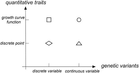
FIGURE 1. Research status on quantitative traits and genetic variants.
GWASs were mainly divided into two types of studies for quantitative traits: 1) an association analysis based on common variants and 2) and an association analysis based on rare variants. At present, the single-variant association analysis has always been used by GWAS based on common variants mainly. Many methods were proposed in these studies and made great progress. However, the single-variant association analysis was limited to test rare variants common in high-throughput sequencing (Han and Pan, 2010; Sha et al., 2016). Common variants explained only a small part of genetic variation, and most of the associated sites that controlled complex traits were rare variants (Gibson, 2012; Marouli et al., 2017). A single-variant association analysis often ignored the overall information of gene region that rare variants were located. An association analysis method based on gene region can analyze the combination of the effects of the variant sites in the entire gene region. That method reduced the burden of multiple testing and has larger test power (Neale and Sham, 2004; Wu et al., 2010).
Most association analysis methods based on the gene region were designed for the phenotypic traits at a single time point. These methods were mainly divided into three types: 1) the burden test method based on the idea of merging (Madsen and Browning, 2009; Han and Pan, 2010; Morris and Zeggini, 2010; Price et al., 2010; Lin and Tang, 2011), 2) the variance composition method based on mixture effects (Liu et al., 2007; Kwee et al., 2008; Liu et al., 2008; Wu et al., 2010; Wu et al., 2011; Schifano et al., 2012; Chen et al., 2013), and 3) the method based on a functional data analysis (Luo et al., 2012; Svishcheva et al., 2015; Svishcheva et al., 2016a; Svishcheva et al., 2016b; Li et al., 2020). The current functional data analysis method maintained a discrete state in the direction of quantitative traits at a single time point and treated many discrete SNP sequences located in a narrow gene region as continuous variables in the direction of the gene locus. Then, gene regions that contained a large amount of genetic variation were analyzed using a functional data analysis (as shown with a triangle in Figure 1). Many studies have shown that the test power of the functional data analysis method was higher than that of the burden test method based on the combination idea and the variance component method based on the mixture effect (Luo et al., 2012; Fan et al., 2013; Svishcheva et al., 2016a).
The literature on the statistical method of the gene region association analysis for longitudinal traits was limited (Beyene and Hamid, 2014; Wu et al., 2014; Yan et al., 2015; Chien et al., 2016; Cao et al., 2017). In recent studies, a longitudinal trait association test method with the covariates based on SKAT (the sequence kernel association test) method (LSKAT; Longitudinal SNP-set/SKAT) was proposed (Wang et al., 2017). This method combined the features of linear mixed models and kernel machine methods. The association between genetic variation regions and longitudinal traits was analyzed using LSKAT. At the same time, a longitudinal trait burden test (LBT) that tested the association between traits and burden scores in a linear mixed model was proposed in that study. However, the inversion of the correlation matrix was required for these methods, and the calculation of the p-value using the eigenvalue decomposition of the correlation matrix brought a computational burden. Simultaneously, the time-varying genetic effect was not considered, but the influence of genes on traits might change over time.
In the functional data analysis, the function-on-function regression model can fit the growth curve of quantitative traits and transform dense discrete gene loci into continuous functions (as shown with a dot in Figure 1). Therefore, we propose a longitudinal functional data association test (LFDAT) method where the function-on-function regression model is applied to detect the association between the gene region and the longitudinal trait. This method can aggregate the small effects distributed at multiple sites, gather the association information of the entire gene region, and improve the test power of related sites with micro effects.
2 Methods
2.1 Function-On-Function Regression Model
Suppose that there are n individuals in a population, and the group structure and other factors are not considered. The SNP sequence constitutes the gene region [0, M] containing the L genetic locus, and the growth and development traits are measured in the time period [0, T]. Let
where
where
2.2 Parameter Estimation
The intercept function
The asterisk is dropped in what follows to further simplify the expression.
Let
Combine (4) and (3) to obtain the following:
where
In simplifying the notations, we further obtain the matrix expression of Eq. 5:
where
The least-square method is used to estimate the coefficient vector
This is equivalent to solving the following equation:
We impose a roughness penalty term on the two-dimensional basis function in each dimension separately.
Let
where
The same, the matrix expression of
where
Now, we wish to minimize the sum of two penalties and the sum of integrated squared errors, expressed as follows:
This is equivalent to solving the following equation:
We evaluate
Let
Then, the regular equation of the least square method can be obtained from Eq. 12
Finally, the least square estimate of the coefficient vector in Eq. 13 is as follows:
2.3 Hypothesis Testing Based on the Function-On-Function Regression Model
We usually consider the following hypothesis testing to detect whether the association between the gene regions and the phenotypes exists:
Since the time-varying function of the genetic effect
The following test statistics are available for the above hypothesis testing:
where
2.4 The Evaluation Indicators of the Estimation Result of the Time-Varying Function of the Genetic Effect
This was done to further measure the fitness of LFDAT for the time-varying function of the genetic effect in the gene region and provide other reference indicators for LFDAT in the process of the association analysis of the longitudinal trait. Then, some evaluation indicators are established for LFDAT.
Let
and
From a statistical genetic point of view, if the time-varying function of the genetic effect
For the null region and non-null region, as Lin et al. (2017) and Centofanti et al. (2020) noted, we consider the integrated squared errors (ISE) as the fitting criterion for the estimator
and
where
The predictive performance is measured by prediction mean squared errors (PMSE), defined as the following:
where test denotes the test sample data set, N is the size of the test sample data set, and
In the gene region, we define ISE0, ISE1, and PMSE as the criterion to measure the fitness of the time-varying effect function. ISE0 is used to measure the fitness of the null effect, which denotes the overall deviation between the true value and the estimated value at the site where there is no effect value in the gene region. The expression is as follows:
where
ISE1 is used to measure the fitness of the non-null effect, which denotes the overall deviation between the true value and the estimated value at the site where there is an effect value in the gene region. The expression is as follows:
where
PMSE is used to measure the fitness of the genetic model, which denotes the overall deviation between the estimated value of the trait obtained fitted by the model and the true value of the trait in the test set. The expression is as follows:
where test denotes the test sample data set, N is the size of test sample data set,
3 Simulation Studies
The SNP sequence data set generated by the computer is used for type I error simulation and power simulation to evaluate the feasibility of the LFDAT. In Luo et al. (2012), the FLM and the Smoothed FLM are proposed for test association between gene region and quantitative trait. Because both the Smoothed FLM and LFDAT have the smooth penalty, so we compare the power of the Smoothed FLM to that of the LFDAT in simulation. However, the Smoothed FLM is only applicable to a single measurement, it’s applied to detect association between gene region and trait at each time point.
In the simulation, we consider linkage equilibrium simulation and linkage disequilibrium simulation. The SNP sequence data set simulated contains a 50 kb gene region, and a 1 kb genetic subregion is randomly selected from the gene region to assess type I error rates and power. The sizes of the samples are 1,000, 1,500, and 2,000, respectively. Gene regions consider five cases: 1) gene regions only have common variants, 2) gene regions only have rare variants, 3) gene regions only have low-frequency variants, 4) gene regions are randomly composed of 20% common variants and 80% rare variants, and 5) gene regions are randomly composed of 80% common variants and 20% rare variants. In the simulation, the upper limit b and lower limit a of U (a, b) corresponding to the MAF (minor allele frequency) of gene regions are different. The gene regions of rare variants are (0.0005, 0.01), gene regions of low-frequency variants are (0.01, 0.05), and gene regions of common variants are (0.05, 0.5).
The codes used in this paper are the linmod function in the fda package of the R software (Ramsay et al., 2009). In the simulation, set the number of two-dimensional B-spline basis functions K to 15 and the order d to 4. Leave-one-out cross-validation (Ramsay et al., 2009) can be used to select the optimal parameter from a set of smoothing coefficients
Due to space limitations, all the simulated results are attached to Supplementary Datas S1–S6.
3.1 Linkage Equilibrium Simulation
3.1.1 Type I Error Rates
We use the following model to generate phenotype data to assess type I error rates of LFDAT:
where
A total of 1,000 genotype-phenotype data sets for each sample size were simulated. The test statistics and related p-value based on the above genetic model were calculated. Under a given significance level α, the ratio of genotype-phenotype data sets that p-value is less than α is regarded as a type I error rate.
All results of type I error rates simulation can be seen Supplementary Data S1. Table 1 shows the type I error rates of the LFDAT and Smoothed FLM at the significance level of 0.05, 0.01, and 0.001 for linkage equilibrium simulation. It can be seen that LFDAT controls the type I error rates at each level of significance. The type I error rates of rare gene regions and low-frequency gene regions are lower than that of common gene regions. The type I error rates of gene regions with more common variants are generally higher than those with less common variants. As the significance level increases, the type I error rates of gene regions gradually decrease. For smaller significance levels (α is 1e-4, 1e-5, and 1e-6), LFDAT still performs well, and the type I error rates are all 0 (See Supplementary Data S1). Compared with the type I error rates of the LFDAT, the type I error rates of the Smoothed FLM is severely inflated. It means that there are more false associated gene regions with quantitative trait using the Smoothed FLM method. Simulation studies have shown that association analysis which combines the multiple measurement of quantitative traits can reduce the type I error rates.
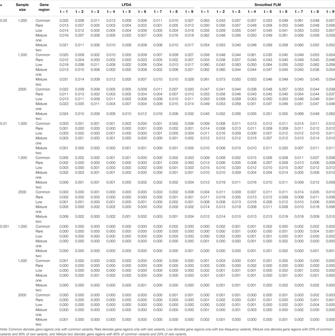
TABLE 1. Type I error rates of the LFDA and Smoothed FLM based on 1,000 simulated replicates for linkage equilibrium simulation.
3.1.2 Power
We randomly selected a 1 kb subregion from the SNP sequence data set under the alternative hypothesis as the genotype data of the variant region to measure the test power of LFDAT for the gene regions. The generate phenotypic data is based on the following model:
where
Consider the following scenarios for simulations: 1) the proportion of causal variants in the gene regions is 1, 2, or 4%, and 2) the proportion of negative effects of causal variants is 0, 20, 50%. Various processes in life activities are always accompanied by the selective opening and closing of different genes, and some genes are selectively expressed at a certain stage of development. Based on this phenomenon, the following two cases were considered for the time-varying function of the genetic effect:
Case one. The time-varying function of the genetic effect is
Case two. The time-varying function of the genetic effect is
For each setting scenario, 1,000 genotype-phenotype data sets are simulated. At the given significance level α, the ratio of genotype-phenotype data sets with a p-value is less than α are used as power. For each genotype-phenotype data set, the variation area is the same for all individuals in the data set. However, we allow the variation of different data sets to be different.
Case One Simulation
We assess the test power of five gene regions under different sample sizes (n = 1,000, 1,500, 2,000) by LFDAT, and the features that result are the same for each sample size. All results of power simulation can be seen Supplementary Data S1.
The figures of power based on LFDAT at nine time points are also shown in Supplementary Data S1 for different significance levels, constant c, the proportion of negative effects, and causal variants. Figure 2 (Only show the power figures when c is 3 and a sample size is 2000) show that the power of each time point is different, which might be the unequal value of the time-varying effect function at each time point. As constant c (See Supplementary Data S1) and the proportion of causal variants increase, the power also increases. However, as the proportion of negative effects and significance levels increase, the power gradually decreases. Overall, the power of the five gene regions is higher. We find that whether it is common, rare or low-frequency variants, as the genetic effects increase, the power of testing gene region increases by simulation study. The proportion of negative effects has a smaller impact on the power of mixture gene region one than on the other four gene regions. It may be that the effect values of rare variants are larger than that of common variants, and the offset effects of mixture gene region one are not as much as other regions. The LFDAT is applicable to common variants, rare variants and low-frequency variants.
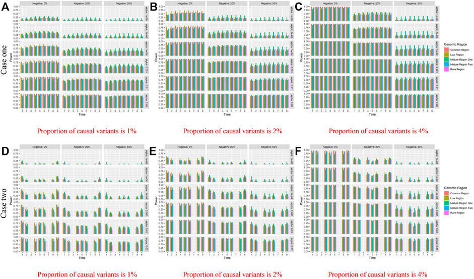
FIGURE 2. Power of linkage equilibrium’s case one and case two based on LFDAT for the five gene regions when c is 3, and sample size is 2000. The (A–C) denotes the power results of case one. The (D–F) denotes the power results of case two. The time effect function is
At the same time, we also compare the power of the LFDAT and Smoothed FLM (See Supplementary Data S1). As the sample size increases, the power increases. In Table 2 (Due to space limitations, results of power are shown when significance level is 0.05, sample is 2000, c is 7, and proportion of causal variants is 1%), we can see that the power of the LFDAT is very close to that of the Smoothed FLM. These results indicate that LFDAT can reduce the probability of making the type I errors with keeping its high power.
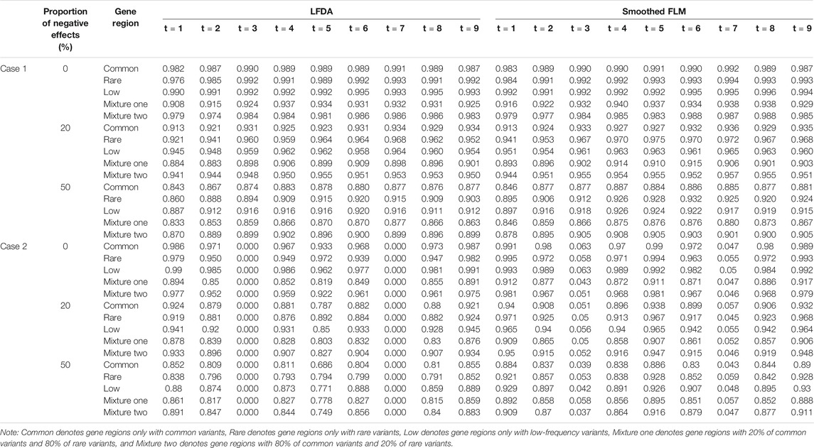
TABLE 2. The power of linkage equilibrium simulation based on LFDA and Smoothed FLM at significance level of 0.05 when sample size is 2000, c is 7 and proportion of causal variants is 1%.
Case Two Simulation
In this case, the time effect function is
3.1.3 Estimation of ISE0, ISE1, and PMSE
We estimate the three evaluation indicators of two cases for five gene regions (See Supplementary Datas S1, S2), and we only display results of case one and case two when c is 3 and a sample size is 2000 in Table 3. In case one and case two simulations for the five gene regions, the means of ISE0 and ISE1 with the gene region of rare variants are the largest. Further, the means of PMSE with the gene region of low-frequency variants are largest in five gene regions. This indicates that LFDAT fits the time-varying effect function better for smaller genetic variants effects. Given the proportion of causal variants and the value of c, the change in the proportion of negative effects has little effect on the means and standard errors of ISE0, ISE1, and PMSE. Meanwhile, the proportion of causal variants and c increases (See Supplementary Datas S1, S2), and the means and the standard errors of ISE0 and PMSE gradually increase, whereas the means and standard errors of ISE1 decrease. The results of case two are smaller than that of case one, which might be affected by gene switching. The time-varying function of the genetic effect is null at a certain time point in case one so that the difference between the estimated time-varying function and the true time-varying function is smaller.

TABLE 3. The means and standard errors (in the parenthesis) of three indicators based on LFDA for linkage equilibrium simulation when sample size is 2000, c is 3
3.2 Linkage Disequilibrium Simulation
The measure of linkage disequilibrium is r2. It is randomly generated from a uniform distribution U (a,b). The measure of linkage disequilibrium between each SNP is not equal. We consider two scenarios that the r2 is between 0.01 and 0.25, and 0.25 and 0.64. Simulation settings of type I error rates and power are the same as Section 3.1. All results of simulation can be seen Supplementary Datas S3–S6. Due to space limitations and the similar features and trends of the results of two scenarios, we only display the partial results of second scenarios (r2 is between 0.25 and 0.64).
Table 4 shows the type I error rates of the LFDAT and Smoothed FLM at the significance level of 0.05, 0.01, and 0.001 for linkage disequilibrium simulation. The part of power results is shown in Table 5 (When significance level is 0.05, sample is 2000, c is 7, and proportion of causal variants is 1%) and Figure 3 (When sample is 2000, and c is 3). Type I error rates of rare gene region and low-frequency gene region are still lower than others. Type I error rates of the LFDAT is still lower than that of the Smoothed FLM, and the type I error rates of the Smoothed FLM is slightly inflated. It is verified once again that the use of the multiple measurement of traits can reduce the probability of making the type I errors. Power of linkage disequilibrium is very high for two cases. Especially in case one, power of five gene regions is 100% when the proportions of the negative effect of causal variants are 0%, 20%. The power of linkage disequilibrium simulation has increased a lot compared with linkage equilibrium simulation, which is due to consider the overall effect together in gene region as loci correlation.
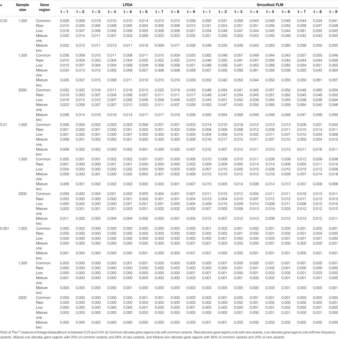
TABLE 4. Type Ⅰ error rates of LFDA and Smoothed FLM based on 1,000 simulated replicates for linkage disequilibrium simulation.
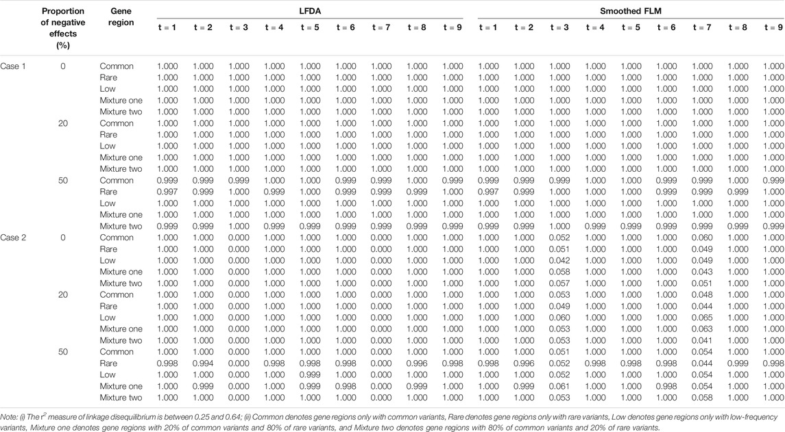
TABLE 5. The power of linkage disequilibrium simulation based on LFDA and Smoothed FLM at significance level of 0.05 when sample size is 2000, c is 7 and proportion of causal variants is 1%.
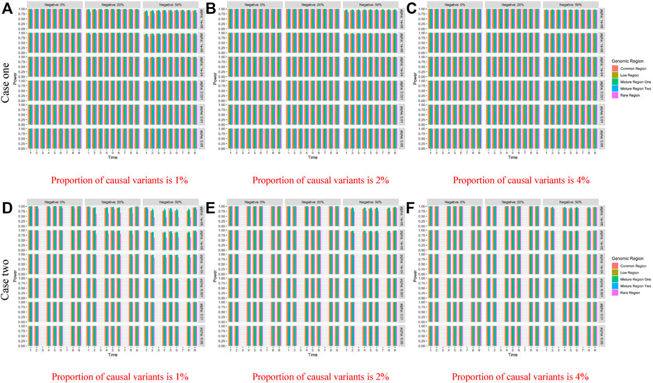
FIGURE 3. Power of linkage disequilibrium’s case one and case two based on LFDAT for the five gene regions when c is 3, and sample size is 2000. The (A–C) denotes the power results of case one. The (D–F) denotes the power results of case two. The time effect function is
At the same time, we evaluate the three indicators of two cases for five gene regions (See Supplementary Datas S3–S6), and here we only display results of case one and case two when c is 3 in Table 6 for second scenarios (r2 is between 0.25 and 0.64). Same as linkage equilibrium simulation, the means of ISE0 and ISE1 of rare gene region is largest and the means of PMSE of rare gene region is smallest. This also verifies that LFDAT fits the time-varying effect function better for smaller genetic effects of gene regions.
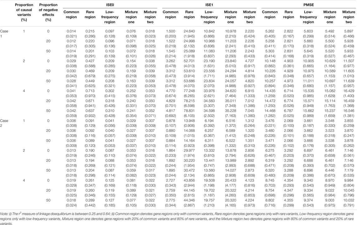
TABLE 6. The means and standard errors (in the parenthesis) of three indicators based on LFDA for linkage disequilibrium simulation when sample size is 2000, c is 3
3.3 Comparison of Simulation
Linkage equilibrium simulation and the two scenarios of linkage disequilibrium simulation are compared and analyzed when sample size is 1,500, constant c is 5, and the proportion of casual variants is 2% (Tables 7–9). The characteristics of the remaining simulation results are similar to that of above simulation. In general, the type I error rates of the two scenarios of linkage disequilibrium simulation is larger than that of linkage equilibrium simulation. This is because the increase in power will increase the type I error rates. From results of two cases we can know that because the r2 measure of linkage disequilibrium increase, the power also increases for five gene regions. The power of linkage disequilibrium simulation is significantly less affected by the proportion of negative effects than that of linkage equilibrium simulation, which is also due to the interaction between genes.
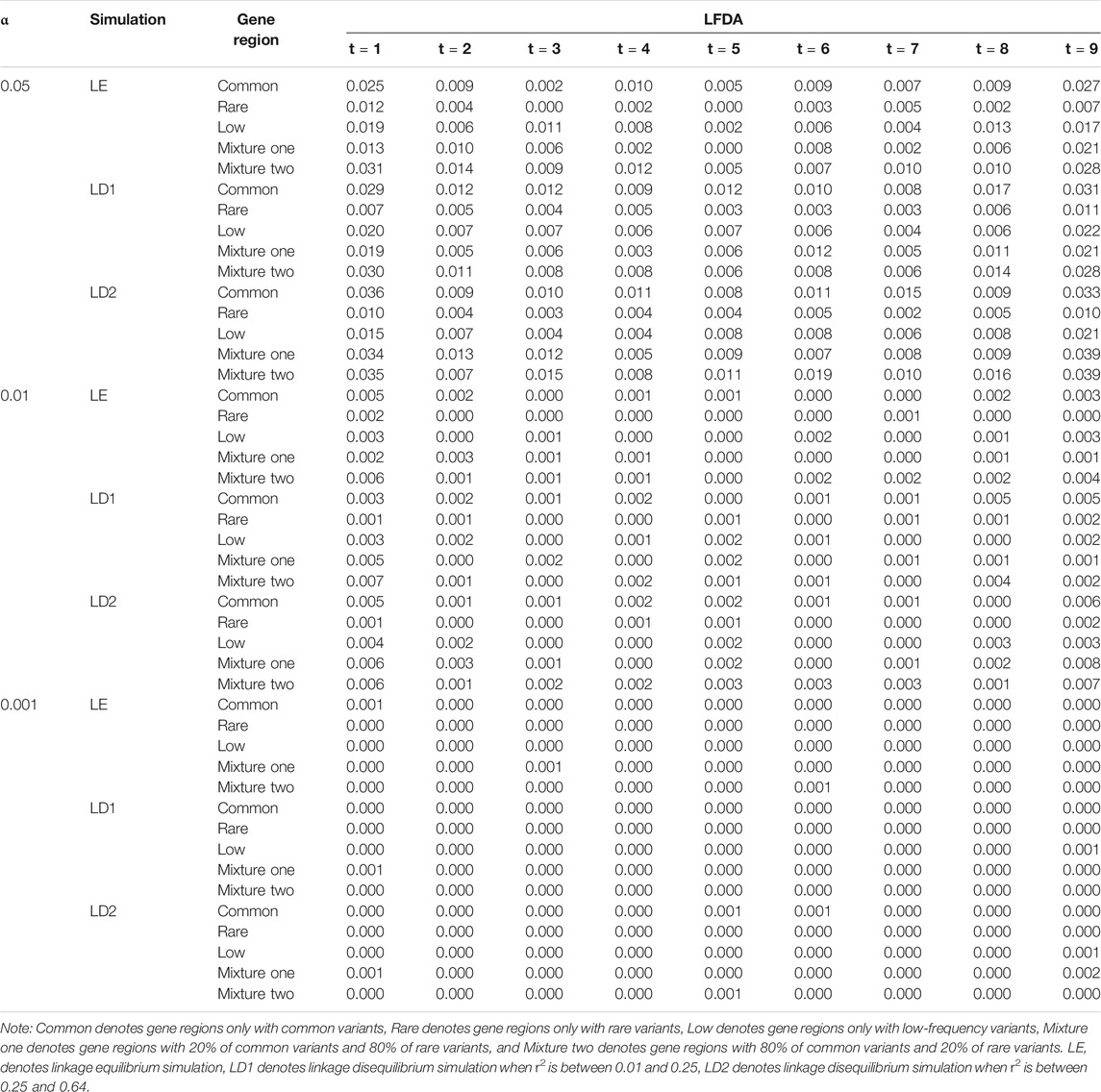
TABLE 7. Compare the type Ⅰ error rates of linkage equilibrium and linkage disequilibrium simulation based on LFDAT when sample size is 1,500.
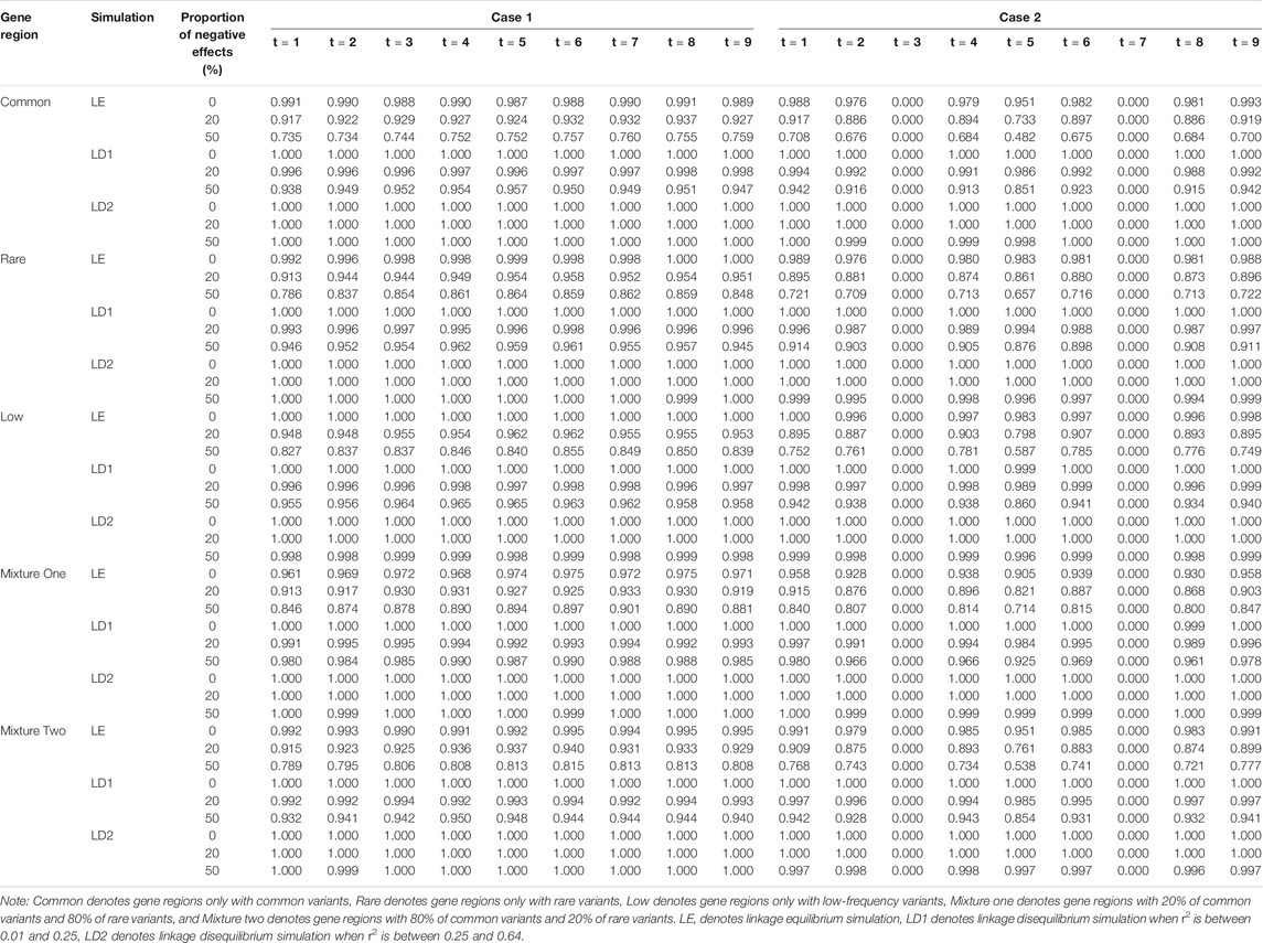
TABLE 8. Compare the power of linkage equilibrium and linkage disequilibrium simulation based on LFDAT when significant level is 0.05, sample size is 1,500, c is 5, and proportion of casual variants is 2%.
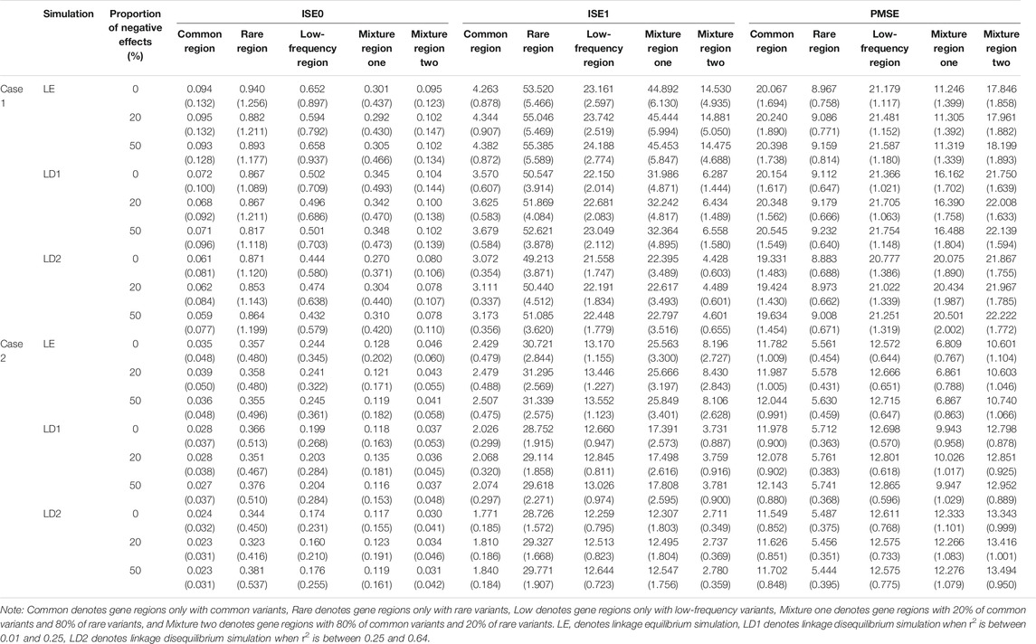
TABLE 9. Compare the estimated means and standard errors (in the parenthesis) of three indicators for linkage equilibrium and linkage disequilibrium simulation based on LFDA method when sample size is 1,500, c is 5, and proportion of casual variants is 2%.
In two cases, as the r2 measure of linkage disequilibrium increase, the means and standard errors of ISE0 of common gene region, low-frequency gene region, and mixture gene region two gradually decrease, and the standard errors of ISE1 of the five gene regions decrease. The means of PMSE of common gene region, rare gene region, and low-frequency gene region first increase and then decrease, but the change is not large. These phenomena may be caused by the fact that the fitting errors of the LFDAT to the time-varying effect function gradually decreases as the r2 measure of linkage disequilibrium increases. Although LFDAT has a little bias for fitting of the time-varying effect function, it does not affect its detection efficiency on a gene region.
In general, LFDAT performs well for both linkage equilibrium and linkage disequilibrium simulations, and has a lower type I error rates with a higher power for gene regions.
4 Application to PSA Data Set
We apply LFDAT to a longitudinal data set (Campbell et al., 2018) of an Oryza sativa projected shoot area (PSA) to demonstrate the applicability of LFDAT. That data set selected 378 lines of RDP1 (Zhao et al., 2011). All experiments were carried on at the Plant Accelerator in the Australian Plant Phenomics Facility at the University of Adelaide, SA, Australia. The experiments were repeated three times from February to April 2016. For details of the experimental design, see Campbell et al. (2018). Briefly, we first transplanted three uniformly germinated seedlings into pots. Seven days after the transplant (DAT), the plants were thinned to one seedling per pot. The plants were imaged daily from 13 to 33 DAT using a red-green-blue camera from two side-view angles, separated by 90° and a single top view. Each experiment adopted a partially replicated design with 54 lines selected randomly, and they were repeated twice. Three experiments produced 73,537 images, and “Plant pixels” were extracted from RGB images using the LemnaGrid software. The sum of the “plant pixels” extracted from the three RGB images is used as an indicator to measure shoot biomass. This indicator is referred to as PSA. PSA has been proved to be an accurate expression of shoot biomass (Golzarian et al., 2011; Campbell et al., 2015; Knecht et al., 2016), which can describe the morphology and dynamic growth of plants.
The first set of data from the first repeated experiment is selected as the phenotypic data, and samples with missing values are eliminated. The 350 samples remaining are used for the subsequent analysis. The development trajectories of the shoot biomass are shown in Figure 4, with the shoot biomass trajectories for all individuals indicated in the background. The genotype data contains a total of 36,901 markers on 12 chromosomes. The missing genotype is estimated, and SNPs with a minimum allele frequency of less than 0.005 are deleted. Finally, 36,058 SNPs remained. In order to be consistent with the results of Campbell et al. (2015), we treat each chromosome as a gene region for the association analysis. The number of SNPs and the p-value of the association analysis of each gene region are shown in Table 10. The correlation coefficients between the measured traits at each time point are close to one. Significant SNP sites have been identified on each chromosome. Further, the SNP sites of chromosome 3 are more significant. In the type I error rates simulation, it can be seen from Table 1 that the type I error rates is low, which indicates that the LFDAT method is less likely to identify false gene region. Therefore, the detection of the significant SNPs on each chromosome is basically credible in our study, which is consistent with the results of Campbell et al. (2015). However, significant SNP sites were not detected at the first two time points. It may be that the PSA growth trajectory is exponentially increasing, and the value is too large, leading to the variation range of PSA being too small at the first and second time points. Then, the difference between the rice populations cannot be identified.
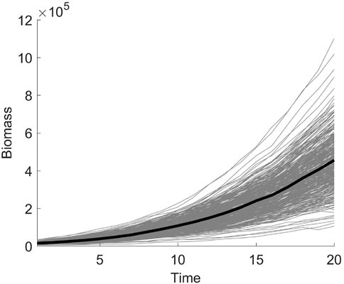
FIGURE 4. The shoot biomass development trajectory of 350 samples. The solid gray line represents the trajectory curve of 350 samples, and the solid black line represents the average trajectory curve.
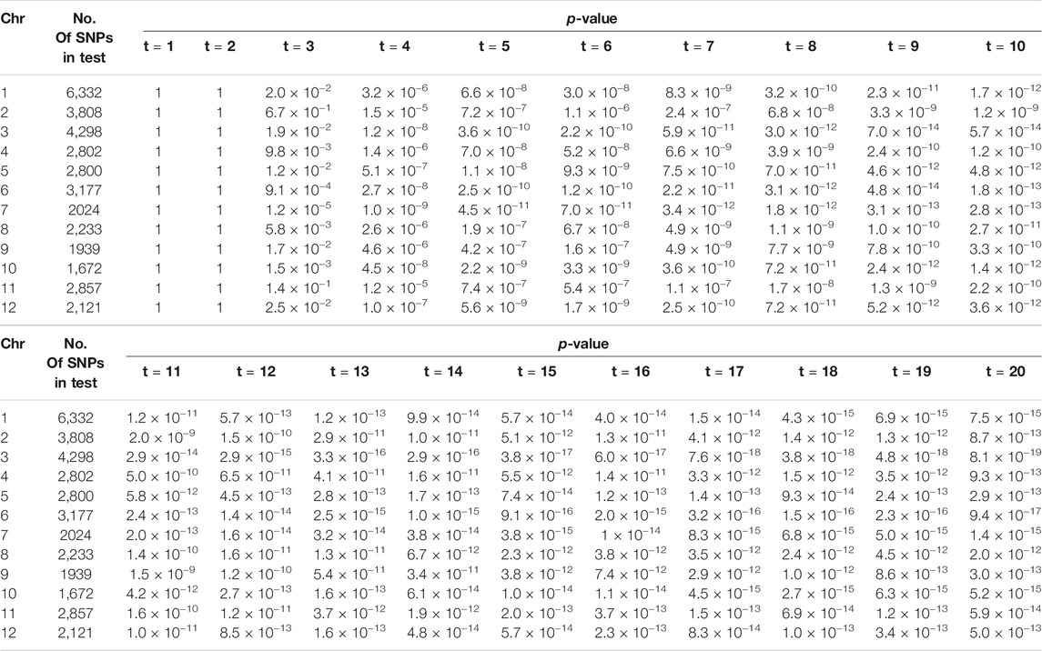
TABLE 10. The number of SNPs and the p-value of the association analysis of each gene region based on LFDAT at significance level of 0.05
The calculation of the whole process was taken 15 s on the Intel Core 3.40 GHz CPU. This result indicates that the genetic region association analysis method based on the LFDAT method is computationally feasible.
5 Discussion
Considering the association analysis of quantitative traits at multiple time points, it is possible to better observe the influence of time-changing genes on quantitative traits. Further, longitudinal trait research based on gene regions can improve the power. We propose the LFDAT method and that the function-on-function regression model is applied to detect the association between gene regions and longitudinal traits. This can simultaneously lead to continuous phenotypic traits and marker information and make full use of the information carried by the traits to explore the influence of genes on longitudinal traits. Compared with other dynamic association analysis methods, the LFDAT method considers the genetic effects of variants in the entire gene region and the time effects of genes. It can also accurately detect the selective expression function of genes. The gene region association analysis based on the LFDAT method has few restrictions on the direction of gene effects, low computational cost, fast detection speed, low false positives, and high power. It further has a stronger explanatory for the effect of genes on the quantitative traits concerning time.
We consider linkage equilibrium simulation and linkage disequilibrium simulation, the powers of the five gene regions are compared to prove the feasibility of LFDAT for a longitudinal trait association analysis in two simulation studies. At the same time, two cases are set for the time-varying function of the genetic effects to explore whether LFDAT can detect the selective expression of genes at different time points. The simulated results show that LFDAT has a lower type I error rates and higher power on the association analysis of the five gene regions and can accurately detect the selective expression of genes in two simulations. In addition, different settings for the variance and correlation coefficient of the random error are simulated. When the variance is 25, compared with the variance of 1, the powers of linkage equilibrium and linkage disequilibrium are significantly reduced, three indicators of linkage disequilibrium increase, and ISE0 and PMSE of linkage equilibrium increase. However, ISE1 of linkage equilibrium decrease. When the correlation coefficient is 0.95, compared with the correlation coefficient of 0.5, power of linkage disequilibrium increase, and three indicators of linkage disequilibrium decrease, however the changes of power and three indicators of linkage equilibrium are not obvious.
For the continuous effect function, we try to plot the figure the estimated time-varying function of the genetic effect in linkage equilibrium and linkage disequilibrium simulation at first time point, in which time effect function and genetic effect function are fixed to constants and causal variants are 55, 66, 77, 88, 99, 110, 121, 132, 143, and 154-th SNP respectively. We find that the fitting of the time-varying function of the genetic effect in the linkage disequilibrium simulation is smoother than that of the linkage equilibrium simulation in most figures (As shown in Supplementary Data S7). This is because there is an association between each SNP, which makes the fitting of the time-varying function more constrained. Furthermore, Haseman and Elston (1972) proposed a linear model for detecting linkage between a marker and a QTL in a full-sib design. Then, the mathematical expectation of the regression coefficient is expressed by the additive genetic variance of the QTL. Chen (2014, 2016) proposed that variance component methods, such as the Haseman-Elston (HE) regression and the linear mixed model (LMM), provide valid estimate of heritability based gene effect in GWAS data for complex traits. The estimated heritability may reveal the genetic architecture underlying a complex trait. For the study about between the heritability and the continuous effect function within a gene region based on functional data analysis, there is currently no relevant research in this field. In the future, we will conduct in-depth research in this direction.
Of course, LFDA that converts gene loci into continuous variables has some shortcomings. First, the covariates, population structure, and locus weights are not considered. In gene regions, the weak effects of rare variants are difficult to find, making it challenging to identify the gene regions of rare variants. The common solution is to assign different weights to different types of variants. In the research on LSKAT and LBT methods proposed by Wang et al. (2017), covariates and population structures were considered, and common and rare variants were given different weights. We sought to study the growth and development mechanism of plants in this paper mainly. However, we could consider adding factors, such as the population structure, and introduce the idea of weight to improve the detection ability of LFDAT in future research.
Second, the fitting errors of indicators ISE0, ISE1, and PMSE are relatively large. It might be because of the limitations of LFDAT, which cannot compress the time-varying function of genetic effects to a state close to null, as stated by Lin et al. (2017). This is one direction of our future research.
Third, in the simulation of the selective gene expression, it can be seen that the powers of linkage equilibrium for five gene region are unstable, and the powers are lower at some time points of the gene opening. We find it is related to the time-varying function of genetic effects by simulating a different time-varying function of the genetic effects. Therefore, accurately grasping how genetic effects change over time is a direction worth studying.
Fourth, for the application on the PSA of the Oryza sativa data set, no significant SNP loci are detected at the first two time points. This indicates that the gene region association analysis based on LFDAT needs to be further improved to make the detection effect more accurate. Then, it could be better applied to the gene region association analysis of different longitudinal traits.
This paper applies the LFDAT method to the real data process, and each chromosome is analyzed as an independent gene region. However, the variants that control longitudinal traits might be distributed in different gene regions. If there is a correlation between the causal variants in different gene regions, it is necessary to perform association analysis on multiple gene regions. This is also true if each chromosome is regarded as a gene region and the region is too large to accurately detect genes that control longitudinal traits. Then, the SNP sequence needs to be refined into multiple gene regions. The extension of the longitudinal trait association analysis based on the functional data analysis to multiple gene regions will be a future research direction.
Data Availability Statement
Publicly available datasets were analyzed in this study. The data can be found here: http://www.ricediversity.org/ and https://doi.org/10.5281/zenodo.1313684.
Author Contributions
YW and SL contributed to the conception of the study; SL performed the simulation studies and the data analysis and wrote the manuscript; SL and SS collected and sorted data; HZ and JS modified the manuscript.
Funding
This work was supported by the National Natural Science Foundation of China (Grant No. 32071892), Natural Science Foundation of Fujian Province of China (Grant No. 2021J01126), Science and Technology Innovation Special Foundation of Fujian Agriculture and Forestry University of China (no.CXZX2020109A).
Conflict of Interest
The authors declare that the research was conducted in the absence of any commercial or financial relationships that could be construed as a potential conflict of interest.
Publisher’s Note
All claims expressed in this article are solely those of the authors and do not necessarily represent those of their affiliated organizations, or those of the publisher, the editors and the reviewers. Any product that may be evaluated in this article, or claim that may be made by its manufacturer, is not guaranteed or endorsed by the publisher.
Acknowledgments
We thank the reviewers for their helpful comments.
Supplementary Material
The Supplementary Material for this article can be found online at: https://www.frontiersin.org/articles/10.3389/fgene.2022.781740/full#supplementary-material
References
Belonogova, N. M., Svishcheva, G. R., Wilson, J. F., Campbell, H., and Axenovich, T. I. (2018). Weighted Functional Linear Regression Models for Gene-Based Association Analysis. PLoS ONE 13, e0190486. doi:10.1371/journal.pone.0190486
Beyene, J., and Hamid, J. S. (2014). Longitudinal Data Analysis in Genome-Wide Association Studies. Genet. Epidemiol. 38, S68–S73. doi:10.1002/gepi.21828
Campbell, M. T., Knecht, A. C., Berger, B., Brien, C. J., Wang, D., and Walia, H. (2015). Integrating Image-Based Phenomics and Association Analysis to Dissect the Genetic Architecture of Temporal Salinity Responses in rice. Plant Physiol. 168, 1476–1489. doi:10.1104/pp.15.00450
Campbell, M., Walia, H., and Morota, G. (2018). Utilizing Random Regression Models for Genomic Prediction of a Longitudinal Trait Derived from High‐Throughput Phenotyping. Plant Direct 2, 1–11. doi:10.1002/pld3.80
Cao, H., Li, Z., Yang, H., Cui, Y., and Zhang, Y. (2017). Longitudinal Data Analysis for Rare Variants Detection with Penalized Quadratic Inference Function. Sci. Rep. 7, 650. doi:10.1038/s41598-017-00712-9
Centofanti, F., Fontana, M., Lepore, A., and Vantini, S. (2020). Smooth Lasso Estimator for the Function-On-Function Linear Regression Model, 00529. arXiv preprint arXiv, 2007.
Chen, G.-B. (2014). Estimating Heritability of Complex Traits from Genome-Wide Association Studies Using IBS-Based Hasemanâ€"Elston Regression. Front. Genet. 5, 1–14. doi:10.3389/fgene.2014.00107
Chen, G.-B. (2016). On the Reconciliation of Missing Heritability for Genome-Wide Association Studies. Eur. J. Hum. Genet. 24, 1810–1816. doi:10.1038/ejhg.2016.89
Chen, H., Meigs, J. B., and Dupuis, J. (2013). Sequence Kernel Association Test for Quantitative Traits in Family Samples. Genet. Epidemiol. 37, 196–204. doi:10.1002/gepi.21703
Chien, L.-C., Hsu, F.-C., Bowden, D. W., and Chiu, Y.-F. (2016). Generalization of Rare Variant Association Tests for Longitudinal Family Studies. Genet. Epidemiol. 40, 101–112. doi:10.1002/gepi.21951
Cousminer, D. L., Berry, D. J., Timpson, N. J., Ang, W., Thiering, E., Byrne, E. M., et al. (2013). Genome-Wide Association and Longitudinal Analyses Reveal Genetic Loci Linking Pubertal Height Growth, Pubertal Timing and Childhood Adiposity. Hum. Mol. Genet. 22, 2735–2747. doi:10.1093/hmg/ddt104
Das, K., Li, J., Wang, Z., Tong, C., Fu, G., Li, Y., et al. (2011). A Dynamic Model for Genome-Wide Association Studies. Hum. Genet. 129, 629–639. doi:10.1007/s00439-011-0960-6
Fan, R., Wang, Y., Mills, J. L., Wilson, A. F., Bailey-Wilson, J. E., and Xiong, M. (2013). Functional Linear Models for Association Analysis of Quantitative Traits. Genet. Epidemiol. 37, 726–742. doi:10.1002/gepi.21757
Fan, R., Zhang, Y., Albert, P. S., Liu, A., Wang, Y., and Xiong, M. (2012). Longitudinal Association Analysis of Quantitative Traits. Genet. Epidemiol. 36, 856–869. doi:10.1002/gepi.21673
Gibson, G. (2012). Rare and Common Variants: Twenty Arguments. Nat. Rev. Genet. 13, 135–145. doi:10.1038/nrg3118
Golzarian, M. R., Frick, R. A., Rajendran, K., Berger, B., Roy, S., Tester, M., et al. (2011). Accurate Inference of Shoot Biomass from High-Throughput Images of Cereal Plants. Plant Methods 7, 2. doi:10.1186/1746-4811-7-2
Han, F., and Pan, W. (2010). A Data-Adaptive Sum Test for Disease Association with Multiple Common or Rare Variants. Hum. Hered. 70, 42–54. doi:10.1159/000288704
Haseman, J. K., and Elston, R. C. (1972). The Investigation of Linkage between a Quantitative Trait and a Marker Locus. Behav. Genet. 2, 3–19. doi:10.1007/BF01066731
Hui, S. L., and Berger, J. O. (1983). Empirical Bayes Estimation of Rates in Longitudinal Studies. J. Am. Stat. Assoc. 78, 753–760. doi:10.1080/01621459.1983.10477015
Kheiralla, A. I., and Whittington, W. J. (1962). Genetic Analysis of Growth in Tomato: The F1 Generation. Ann. Bot. 26, 489–504. doi:10.1093/oxfordjournals.aob.a083808
Knecht, A. C., Campbell, M. T., Caprez, A., Swanson, D. R., and Walia, H. (2016). Image Harvest: An Open-Source Platform for High-Throughput Plant Image Processing and Analysis. J. Exp. Bot. 67, 3587–3599. doi:10.1093/jxb/erw176
Kwee, L. C., Liu, D., Lin, X., Ghosh, D., and Epstein, M. P. (2008). A Powerful and Flexible Multilocus Association Test for Quantitative Traits. Am. J. Hum. Genet. 82, 386–397. doi:10.1016/j.ajhg.2007.10.010
Laird, N. M., and Ware, J. H. (1982). Random-effects Models for Longitudinal Data. Biometrics 38, 963–974. doi:10.2307/2529876
Lee, S., Wu, M. C., and Lin, X. (2012). Optimal Tests for Rare Variant Effects in Sequencing Association Studies. Biostatistics 13, 762–775. doi:10.1093/biostatistics/kxs014
Lewis, E. B. (1978). “A Gene Complex Controlling Segmentation in drosophila,” in Genes, Development and Cancer. Editor H.D. Lipshitz (Boston, MA: Springer), 205–217. doi:10.1007/978-1-4419-8981-9_13
Li, Y., Wang, F., Wu, M., and Ma, S. (2020). Integrative Functional Linear Model for Genome-Wide Association Studies with Multiple Traits. Biostatistics, 1–17. doi:10.1093/biostatistics/kxaa043
Lin, D.-Y., and Tang, Z.-Z. (2011). A General Framework for Detecting Disease Associations with Rare Variants in Sequencing Studies. Am. J. Hum. Genet. 89, 354–367. doi:10.1016/j.ajhg.2011.07.015
Lin, Z., Cao, J., Wang, L., and Wang, H. (2017). Locally Sparse Estimator for Functional Linear Regression Models. J. Comput. Graphical Stat. 26, 306–318. doi:10.1080/10618600.2016.1195273
Liu, D., Ghosh, D., and Lin, X. (2008). Estimation and Testing for the Effect of a Genetic Pathway on a Disease Outcome Using Logistic Kernel Machine Regression via Logistic Mixed Models. BMC Bioinformatics 9, 1–11. doi:10.1186/1471-2105-9-292
Liu, D., Lin, X., and Ghosh, D. (2007). Semiparametric Regression of Multidimensional Genetic Pathway Data: Least-Squares Kernel Machines and Linear Mixed Models. Biometrics 63, 1079–1088. doi:10.1111/j.1541-0420.2007.00799.x
Luo, L., Zhu, Y., and Xiong, M. (2012). Quantitative Trait Locus Analysis for Next-Generation Sequencing with the Functional Linear Models. J. Med. Genet. 49, 513–524. doi:10.1136/jmedgenet-2012-100798
Madsen, B. E., and Browning, S. R. (2009). A Groupwise Association Test for Rare Mutations Using a Weighted Sum Statistic. Plos Genet. 5, e1000384. doi:10.1371/journal.pgen.1000384
Malfait, N., and Ramsay, J. O. (2003). The Historical Functional Linear Model. Can. J. Stat. 31, 115–128. doi:10.2307/3316063
Marouli, E., Graff, M., Medina-Gomez, C., Lo, K. S., Wood, A. R., Kjaer, T. R., et al. (2017). Rare and Low-Frequency Coding Variants Alter Human Adult Height. Nature 542, 186–190. doi:10.1038/nature21039
Meirelles, O. D., Ding, J., Tanaka, T., Sanna, S., Yang, H.-T., Dudekula, D. B., et al. (2013). SHAVE: Shrinkage Estimator Measured for Multiple Visits Increases Power in GWAS of Quantitative Traits. Eur. J. Hum. Genet. 21, 673–679. doi:10.1038/ejhg.2012.215
Morris, A. P., and Zeggini, E. (2010). An Evaluation of Statistical Approaches to Rare Variant Analysis in Genetic Association Studies. Genet. Epidemiol. 34, 188–193. doi:10.1002/gepi.20450
Muthen, B. (2004). “Latent Variable Analysis: Growth Mixture Modeling and Related Techniques for Longitudinal Data,” in The Sage Handbook of Quantitative Methodology for the Social Sciences. Editor D. Kaplan (Thousand Oaks, CA: Sage).
Neale, B. M., and Sham, P. C. (2004). The Future of Association Studies: Gene-Based Analysis and Replication. Am. J. Hum. Genet. 75, 353–362. doi:10.1086/423901
Price, A. L., Kryukov, G. V., de Bakker, P. I. W., Purcell, S. M., Staples, J., Wei, L.-J., et al. (2010). Pooled Association Tests for Rare Variants in Exon-Resequencing Studies. Am. J. Hum. Genet. 86, 832–838. doi:10.1016/j.ajhg.2010.04.005
Ramsay, J., Hooker, G., and Graves, S. (2009). Functional Data Analysis with R with Matlab. New York: Springer.
Raudenbush, S. W., and Bryk, A. S. (2002). Hierarchical Linear Models: Applications and Data Analysis Methods. Thousand Oaks, CA: Sage.
Robinson, M. R., Wray, N. R., and Visscher, P. M. (2014). Explaining Additional Genetic Variation in Complex Traits. Trends Genet. 30, 124–132. doi:10.1016/j.tig.2014.02.003
Schifano, E. D., Epstein, M. P., Bielak, L. F., Jhun, M. A., Kardia, S. L. R., Peyser, P. A., et al. (2012). SNP Set Association Analysis for Familial Data. Genet. Epidemiol. 36, 797–810. doi:10.1002/gepi.21676
Sha, Q., Zhang, K., and Zhang, S. (2016). A Nonparametric Regression Approach to Control for Population Stratification in Rare Variant Association Studies. Sci. Rep. 6, 1–12. doi:10.1038/srep37444
Smith, E. N., Chen, W., Kähönen, M., Kettunen, J., Lehtimäki, T., Peltonen, L., et al. (2010). Longitudinal Genome-Wide Association of Cardiovascular Disease Risk Factors in the Bogalusa Heart Study. Plos Genet. 6, e1001094. doi:10.1371/journal.pgen.1001094
Svishcheva, G. R., Belonogova, N. M., and Axenovich, T. I. (2015). Region-Based Association Test for Familial Data under Functional Linear Models. PLoS ONE 10, e0128999. doi:10.1371/journal.pone.0128999
Svishcheva, G. R., Belonogova, N. M., and Axenovich, T. I. (2016b). Some Pitfalls in Application of Functional Data Analysis Approach to Association Studies. Sci. Rep. 6, 1–7. doi:10.1038/srep23918
Svishcheva, G. R., BelonogovaAxenovich, N. M. T. I., and Axenovich, T. I. (2016a). Functional Linear Models for Region-Based Association Analysis. Russ. J. Genet. 52, 1094–1100. doi:10.1134/S1022795416100124
Tang, W., Kowgier, M., Loth, D. W., Soler Artigas, M., Joubert, B. R., Hodge, E., et al. (2014). Large-Scale Genome-Wide Association Studies and Meta-Analyses of Longitudinal Change in Adult Lung Function. PLoS ONE 9, e100776. doi:10.1371/journal.pone.0100776
Wang, Z., Xu, K., Zhang, X., Wu, X., and Wang, Z. (2017). Longitudinal SNP-Set Association Analysis of Quantitative Phenotypes. Genet. Epidemiol. 41, 81–93. doi:10.1002/gepi.22016
Wu, M. C., Kraft, P., Epstein, M. P., Taylor, D. M., Chanock, S. J., Hunter, D. J., et al. (2010). Powerful SNP-Set Analysis for Case-Control Genome-wide Association Studies. Am. J. Hum. Genet. 86, 929–942. doi:10.1016/j.ajhg.2010.05.002
Wu, M. C., Lee, S., Cai, T., Li, Y., Boehnke, M., and Lin, X. (2011). Rare-Variant Association Testing for Sequencing Data with the Sequence Kernel Association Test. Am. J. Hum. Genet. 89, 82–93. doi:10.1016/j.ajhg.2011.05.029
Wu, Z., Hu, Y., and Melton, P. E. (2014). Longitudinal Data Analysis for Genetic Studies in the Whole-Genome Sequencing Era. Genet. Epidemiol. 38, S74–S80. doi:10.1002/gepi.21829
Yan, Q., Weeks, D. E., Tiwari, H. K., Yi, N., Zhang, K., Gao, G., et al. (2015). Rare-Variant Kernel Machine Test for Longitudinal Data from Population and Family Samples. Hum. Hered. 80, 126–138. doi:10.1159/000445057
Zhang, Y. M. (2006). Research Progress on Crop QTL Mapping Method. Chin. Sci. Bull. 51, 2223–2231. (Chinese). doi:10.1007/s11434-006-2201-2
Zhao, B. (2015). How Does Climate Change Affect forest Fire Rate in British Columbia? B.Sc.Thesis. Vancouver: University of British Columbia.
Keywords: association testing, functional data analysis, longitudinal traits, gene region, rare variants
Citation: Li S, Li S, Su S, Zhang H, Shen J and Wen Y (2022) Gene Region Association Analysis of Longitudinal Quantitative Traits Based on a Function-On-Function Regression Model. Front. Genet. 13:781740. doi: 10.3389/fgene.2022.781740
Received: 23 September 2021; Accepted: 04 January 2022;
Published: 21 February 2022.
Edited by:
Hailan Liu, Maize Research Institute of Sichuan Agricultural University, ChinaReviewed by:
Shibo Wang, University of California, Riverside, United StatesGuo-Bo Chen, Zhejiang Provincial People’s Hospital, China
Copyright © 2022 Li, Li, Su, Zhang, Shen and Wen. This is an open-access article distributed under the terms of the Creative Commons Attribution License (CC BY). The use, distribution or reproduction in other forums is permitted, provided the original author(s) and the copyright owner(s) are credited and that the original publication in this journal is cited, in accordance with accepted academic practice. No use, distribution or reproduction is permitted which does not comply with these terms.
*Correspondence: Yongxian Wen, wenyx9681@fafu.edu.cn