Enhancing data-driven soil moisture modeling with physically-guided LSTM networks

1 Introduction

Soil moisture (SM) is a pivotal variable within the climate system, exerting profound influences on water, energy, and biogeochemical cycles. Its involvement in global-scale feedback mechanisms renders it crucial for climate change prediction (Seneviratne et al., 2010; Yamazaki et al., 2017). In the agricultural sector, there is potential for enhancing irrigation schemes (Ying et al., 2016), and mitigate the proliferation of agricultural pests and water pollution (Rosenzweig et al., 2001). In hydrology, soil moisture serves as a valuable indicator for refining parameterization schemes related to land surface models for hydrological processes (Brocca et al., 2017), and shapes the performance of physical models and the assessment of wet and dry conditions (Walker et al., 2009). Additionally, soil moisture assumes a critical indicative role in climate change dynamics (Solomon et al., 2007). However, the significant spatial and temporal heterogeneity characterizing soil moisture variability, governed by diverse factors including soil properties, precipitation, and vegetation, presents a formidable challenge for accurate soil moisture forecasting (Thober et al., 2015). Over the past decades, researchers have endeavored to develop various models to capture the trends in soil moisture variability. These models can broadly be classified into two categories: physical process-based models (Penman, 1948; Thornthwaite, 1948; Chopart and Vauclin, 1990; Henderson-Sellers, 1996; Eltahir, 1998; Kroes et al., 2000) and data-driven empirical models (Fang et al., 2019; Diouf et al., 2020; Li et al., 2021, 2022a,b, 2023).

Models grounded in physical processes typically encompass land surface models and hydrological models. Land surface models employ meteorological forcing datasets (comprising precipitation, temperature, specific humidity, surface pressure, radiation, wind speed, etc.) to simulate physical processes through partial differential equations. However, they heavily rely on data, rendering them susceptible to inaccuracies in meteorological forcing data, which consequently yield erroneous outcomes (Cosgrove et al., 2003). Hydrological models, on the other hand, consider water inputs (e.g., rainfall, irrigation) and outputs (e.g., evaporation, runoff) along with storage (water content in the soil) to predict changes in soil moisture. These models solve equations based on physical processes, such as the water balance equation and energy balance equation (Penman, 1948; Thornthwaite, 1948; Kroes et al., 2000). However, the accuracy of hydrological models hinges on the representation of system responses through the model structure and the reliability of the data utilized (Beven, 2006). In summary, a prominent limitation of physical process-based models lies in the empirical approach employed to determine key parameters, resulting in substantial uncertainties in the model results, particularly when applied at a global scale (Lazer et al., 2014).

In recent years, the rapid advancement of computer hardware has paved the way for data-driven models, notably Deep Learning (DL) approaches. Among these approaches, Long Short-Term Memory (LSTM) networks have demonstrated exceptional capacity for nonlinear fitting. LSTM networks effectively capture and manage long-term dependencies through the integration of gating mechanisms and memory cells. This characteristic makes them particularly suitable for handling short-term memory in soil moisture forecasting. Consequently, LSTM models have gained wide popularity in the field. For instance Fang et al. (2017) employed an LSTM model to predict surface soil moisture based on climate forcing data and geographic attributes such as soil texture and terrain slope. The model exhibited impressive performance, achieving a low test root mean square error (RMSE) of approximately 0.035 and a high correlation coefficient of approximately 0.87 over more than 75% of the continental U.S. Two years later, Fang et al. (2019) further enhanced their predictions by incorporating additional land surface attribute variables (e.g., topography, vegetation type, land surface roughness) to fuse LSTM and land surface process model (Noah) calculations through mean computation. This fusion approach enabled improved surface soil moisture predictions. In another study, Cai et al. (2019) developed a DL regression network with two hidden layers to establish a prediction model linking meteorological parameters to soil moisture at a depth of 20 cm in the Yanqing area of Beijing, China. The model achieved an impressive determination coefficient correlation of 98%. Diouf et al. (2020) utilized data from the European Centre for Medium-Range Weather Forecasts 5th Generation Land Surface Reanalysis Dataset (ERA5-Land) specific to the West Africa region. They constructed a deep neural network comprising two sequentially connected hidden layers to successfully predict soil moisture in layers 1 and 2 for the subsequent 2 to 7 days. The average absolute error ranged between 0.01 and 0.03 m³/m³, demonstrating low prediction discrepancies.

Li et al. (2022a) incorporated a transfer learning approach into three types of DL prediction models: spatial models based on convolutional structures, temporal models based on LSTM structures, and spatio-temporal models based on ConvLSTM structures. They used 3-day lagged meteorological forcing data (specifically rainfall) and land surface variables (soil temperature and soil moisture) to enhance surface soil moisture prediction accuracy after 3–7 days. This approach aimed to alleviate the issue of overfitting during DL training, which can arise due to limited data availability. The following year Li et al. (2022b) further advanced their predictions by utilizing 10-day lagged meteorological forcing data (rainfall, long wave radiation, short wave radiation, atmospheric temperature, atmospheric pressure, and wind speed), land surface variables (soil temperature and soil moisture), and temporal statistical variables (values representing days and months of the year). They designed an LSTM model with a multi-feature attention mechanism, enabling soil moisture predictions at a depth of 10 cm for 1 to 7 days. Notably, this model yielded interpretable results that explained the changing importance of variables during the training process. Collectively, the aforementioned studies illustrate that DL models are particularly suited for handling high-dimensional, nonlinear, and complex meteorological data.

However, “pure” DL models also encounter certain challenges and frequently lack traceability to fundamental physical laws (Dueben and Bauer, 2018). To address this issue, researchers have started exploring the integration of scientific knowledge into DL models (Willard et al., 2022). This integration can be achieved through three main approaches: (1) employing physical knowledge-constrained DL loss functions (Karpatne et al., 2017; Read et al., 2019; Kahana et al., 2020; Zhang et al., 2020; Jia et al., 2021; Xie et al., 2021), (2) utilizing simulation results from physical models to guide the initialization of DL parameters (Read et al., 2019; Jia et al., 2021; Xie et al., 2021), and (3) designing DL model structures that ensure their simulation results are physically consistent (Karpatne et al., 2017; Zhang et al., 2020).

Physical knowledge constraints on the loss function of a DL model can guide its predictions to be consistent with physical principles. By incorporating physical constraints for regularization, the search space for model parameters can be reduced, constraining the model to adhere to physical laws. This approach ensures the model’s consistency with the laws of physics throughout the optimization process. Compared to traditional DL models, DL models with physical constraints demonstrate improved generalization performance and greater robustness when faced with unseen samples (Read et al., 2019; Jia et al., 2020). For instance, Kahana et al. (2020) introduced a method that integrates the solution of the fluctuation equation into a neural network, incorporating physical information. By penalizing the model based on the physical understanding of the fluctuation equation, more accurate and robust results can be achieved, with the IOU score decreasing from 66 to 35% in the absence of noise.

On the other hand, Zhang et al. (2020) trained a CNN model using a limited dataset and physical constraints. The laws of dynamics were utilized to provide constraints on the network output and mitigate the overfitting problem. By comparing the predictions of both physically constrained and unconstrained CNN models, the correlation coefficients of the predicted displacement time series on four different datasets were found to be 0.95, 0.92, 0.87, 0.61 (PhyCNN prediction) and 0.60, 0.72, 0.66, 0.37 (CNN prediction), respectively.

Xie et al. (2021) demonstrated that a DL model incorporating physical mechanisms exhibited a strong explanatory power for extreme events and monotonic relationships in rainfall-runoff simulations. They further enhanced the model’s performance and optimization objectives by introducing synthetic samples and external loss functions. As a result, the average Nash-Sutcliffe efficiency (NSE) for daily simulations during local model testing improved from 0.52 to 0.61.

Karpatne et al. (2017) employed the physical relationship between temperature, density, and water depth to formulate a physical loss function, guaranteeing that the density of water at lower depths remained greater than the density of water at any higher depth. In Lake Mendota, the mean test RMSE for the PGNN model were 1.79 and 1.93 with and without the inclusion of the physical constraint, respectively. The corresponding physical inconsistency scores, which indicate the percentage of time steps in which the density-depth relationship was violated, were 0 and 0.33, respectively.

However, when it comes to predicting large-scale soil moisture with spatial and temporal consistency, physically constrained DL models face challenges due to the varying sensitivity of soil moisture predictors across different regions (Luo et al., 2022). Designing globally applicable physically constrained loss functions and utilizing them as guides for DL models is a challenging task. In this study, we aim to explore the effectiveness of physically constrained loss functions for soil moisture forecasting. Specifically, we propose two physically based loss functions based on the principle of surface water balance, which captures the cyclic relationship between rainfall (inflow water), evapotranspiration (outflow water), and soil moisture (stored water).

These include the design of two monotonic loss functions: one based on the monotonic relationship between inflow water minus outflow water and surface soil moisture and another based on the monotonic relationship between inflow water minus outflow water and deep soil water. The monotonic loss functions are designed to reflect the behavior of soil moisture, wherein its values increase with an increase in inflow water and decrease with an increase in outflow water during changes in moisture states.

In this study, we employ these two physically constrained loss functions as guides for training the DL model. By integrating physical principles into the loss functions, we aim to enhance the model’s ability to learn and represent the underlying physical processes governing soil moisture dynamics.

2 Methods

2.1 Data sources

Prior research has indicated that employing atmospheric forcing data and static terrain attributes (surface model parameters) as inputs for DL models yields highly accurate soil moisture representations. Atmospheric forcing data encompasses variables such as precipitation, temperature, radiation, humidity, and wind speed, while static terrain attributes refer to soil texture, soil moisture capacity, and land cover (Feng et al., 2020; Li et al., 2023).

We previously established the LandBench dataset for predicting surface variables. This dataset includes a wide range of global variables from the ERA5-Land, ERA5 reanalysis, SoilGrid, SMSC, and MODIS datasets. The data has been processed into daily records at resolutions of 0.5°, 1°, 2°, and 4° for application in data-driven models (Feng et al., 2020; Li et al., 2024). In this study, we utilize data with a resolution of 0.5°.

Our training objective involves predicting soil moisture (0–7 cm) sourced from the ERA5-Land reanalysis dataset. Meteorological forcing data (including precipitation, longwave radiation, specific humidity, surface pressure, downward shortwave radiation, surface temperature, and wind speed) and static attribute data (land cover, soil water-holding capacity, elevation data, and soil texture) serve as input features for the deep learning model. Land surface variable data (including soil moisture, evapotranspiration, runoff, and snow accumulation within the range of 7–100 cm) are also incorporated into the loss function design. Meteorological forcing and land surface variable data are sourced from the ERA5-Land reanalysis dataset, land cover data from Friedl et al. (2010), soil water-holding capacity data from the SMSC dataset (Xie et al., 2022), elevation data from the MERIT DEM (Yamazaki et al., 2017), and soil texture data (represented by parameters denoting sand, silt, and clay content) from the SoilGrid dataset.

2.2 Long short-term memory networks

We have adopted Long Short-Term Memory networks (LSTM) (Hochreiter and Schmidhuber, 1997) as the modeling framework for our model. In comparison to traditional Artificial Neural Networks (ANNs), Recurrent Neural Networks (RNNs) demonstrate the ability to effectively capture the relationship between the current time step and previous time steps in time series data. However, RNNs encounter challenges in preserving long-term dependencies within the input sequence when the distance between correlated information across time steps increases. To address the issue of gradient vanishing or exploding in RNNs, LSTM networks were developed. LSTMs incorporate a gating mechanism that enables the effective storage and transfer of long-term dependency information, resulting in improved handling of time series data.

The LSTM architecture (Figure 1) processes a sequence of input features x = [ $x\left[1\right]$ ,…, $x\left[\mathrm{T}\right]$ ] spanning T time steps. Each element $x\left[t\right]$ represents a vector containing features at time step t. A vector of recurrent cell states $c\left[t\right]$ is updated based on the input features and the current cell state values at time t. These cell states also determine the LSTM outputs or hidden states $h\left[t\right]$ . The hidden states $h\left[t\right]$ are then passed through a head layer, where they are combined to generate predictions y[t] that aim to match the target data. The specific structure of LSTM is shown in Equations 1–7:

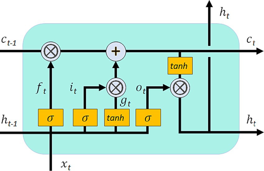
Figure 1. The individual time steps of a standard LSTM model. At each time step t, the model incorporates input features x_t, cell states c_t, and cyclic inputs h_t. The forgetting gate f_t, input gate i_t, and output gate o_t are employed to control the flow of information. Additionally, the cell input g_t is utilized. The boxes labeled σ and tanh represent a single Sigmoid activation layer and hyperbolic tangent activation layer, respectively, both containing the same number of nodes as the cell state. The symbol “+” signifies element-wise summation, while “ $\otimes$ ” denotes element-wise multiplication.

In the LSTM architecture, the symbols $\mathrm{i}\left[t\right]$ , $f\left[t\right]$ , and $o\left[t\right]$ represent the input, forgetting, and output gates, respectively. The gate $g\left[t\right]$ corresponds to the cell input, $x\left[t\right]$ represents the network input at time step t, $h\left[t-1\right]$ is the output of the LSTM (referred to as the cyclic input), and $c\left[t-1\right]$ denotes the cell state from the previous time step.

The cell state serves as the memory of the system at the current time and is initially set to an all-zero vector. The Sigmoid activation function $\sigma \left(\text{.}\right)$ is applied to constrain the values within the range of [0, 1]. These Sigmoid functions are employed in the forgetting, input, and output gates, analogous to the on/off states of switches. Multiplying any value by [0, 1] corresponds to a decay operation. The forgetting gate determines the time scale of memory for each cell state, while the input and output gates control the information flow from the input features to the cell state and from the cell state to the output (cyclic input), respectively.

The calibrated parameters W, U, and b are associated with specific gate matrices/vectors, as indicated by the subscripts. The hyperbolic tangent activation function tanh(·) introduces non-linearity and is used in the cell input and cyclic input. The symbol $\otimes$ denotes element-by-element multiplication. Finally, ${\hat{y}}_t$ represents the predicted value of the soil moisture.

The theoretical foundation of our model is rooted in the fundamental principle of mass conservation. The conservation of mass is a crucial law in water balance models and hydrological model implementations, serving as a pivotal element in assessing the physical validity of soil moisture predictions. To ensure the adherence to this principle, we have devised two loss functions based on the water balance concept. These loss functions will serve as guidance in training the LSTM model. The integration of these aforementioned components constitutes the core framework of our study (see Figure 2).

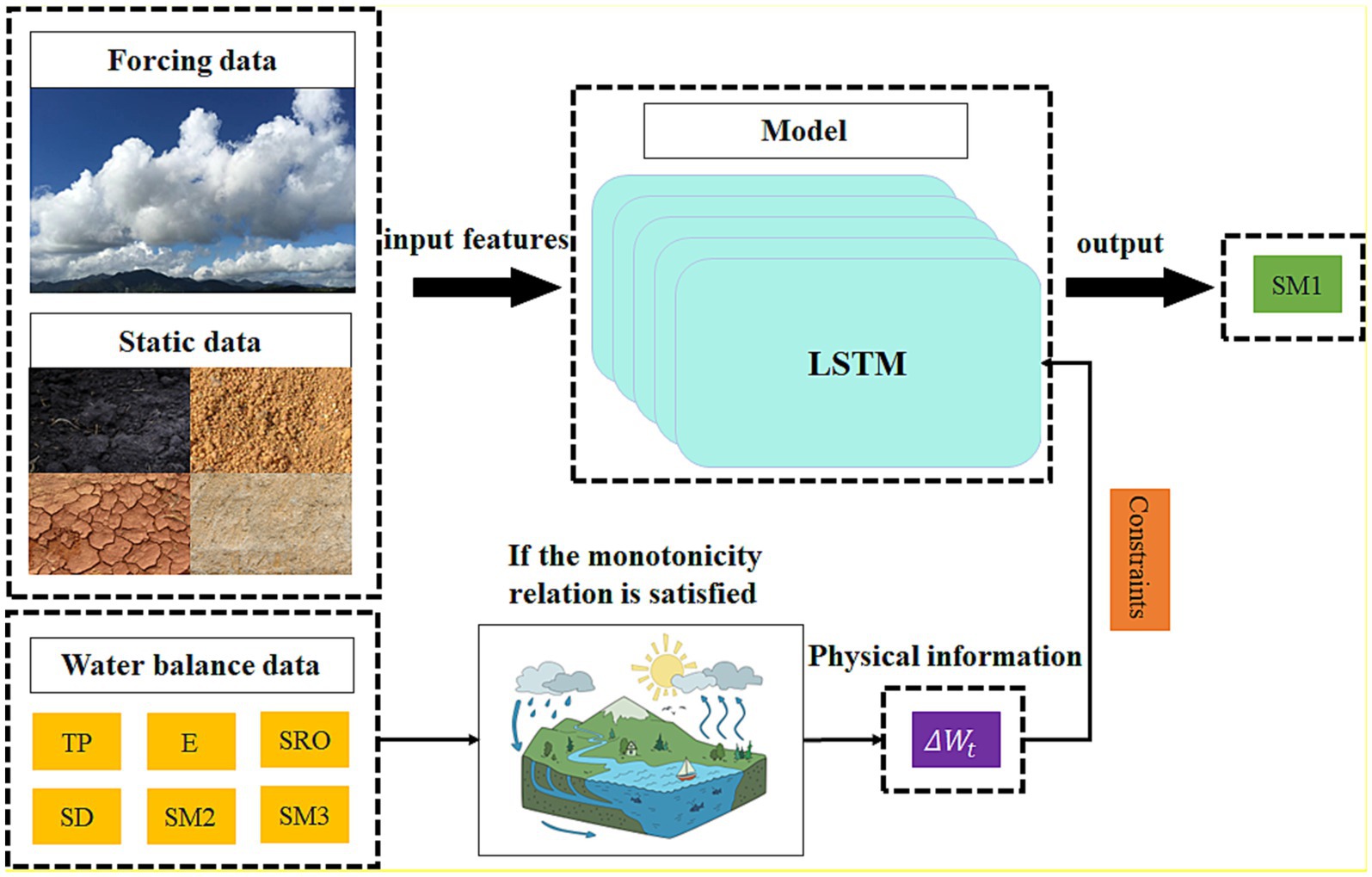
Figure 2. Flowchart of building a land surface water model using the physically guided LSTM network. This figure illustrates the process of establishing a land surface water model using the Physically Guided LSTM network, where meteorological forcings and static variables are used as input features. Within the process, data that adheres to monotonic relationships is selected and included in the calculation of the physical loss term.

2.3 Model training and parameter adjustment

This study focuses on a global scale (excluding Antarctica). Given the relatively high resolution and large dataset, the study adopted a point sampling training method as proposed by Fang and Shen (2020), significantly enhancing model training speed. The training period spans from January 1, 2018, to December 23, 2019, with 75% of the data used for training and the remaining 25% for validation, progressing in chronological order. The testing period ranges from January 1, 2020, to December 31, 2020. Before the model training commenced, all input features were normalized to expedite convergence. The loss function was defined as the root mean square error (RMSE) between observed values and predictions.

In the parameter adjustment section, reference was made to our previous work (Li et al., 2024). The hyperparameters of the model were set as follows: 1000 epochs, but typically, the model reached its optimal performance after approximately 200–300 epochs. To enhance training efficiency, a validation was performed every 20 epochs, and an early stopping technique was employed to prevent overfitting. When the validation loss did not decrease for ten consecutive validation sets, the model was halted, and the model with the lowest validation loss was saved. The optimizer chosen was the Adam optimizer, the model featured one hidden layer with 128 hidden units, a dropout rate of 0.15, a learning rate of 0.001, and a sequence length of 7. To ensure reproducibility and eliminate the impact of random factors on results, a fixed random seed was employed for weight initialization. The model did not include a warm-up period.

All experiments were conducted on a server equipped with an Intel Core (TM) i9-10980XE, 3.00GHz × 36 CPU, 128GB of memory, and two NVIDIA RTX A5000 graphics cards.

2.4 Methodology

The fundamental concept behind the design of the loss function is to account for the relationship between the change in soil moisture (the difference between the previous time step’s soil moisture and the current time step’s soil moisture) and the water entering the soil (precipitation at the current time step) minus the water leaving the soil (evapotranspiration at the current time step). Ideally, these should be equal (representing absolute water balance, which is challenging to achieve) or exhibit a certain level of correlation with a degree of monotonicity. Specifically, when the amount of water entering the system at the current time-step exceeds that of the previous time-step, soil moisture should increase. Conversely, when the current inflow is less than the previous one, soil moisture should decrease. When there is no significant change in the incoming water, soil moisture variation should also be minimal. Consequently, this study devised two loss functions based on the aforementioned principles. These include the physically monotonic loss function that enforces the physical monotonicity of the changes in soil moisture’s inflow (precipitation, condensation, snowmelt) and outflow (evaporation, runoff), as well as the changes in single-layer and multi-layer soil moisture, as illustrated below:

Equation (8) presents a monotonic loss function designed on the principle of surface water balance in the topsoil. Here, $Los{s}_{\mathit{RMSE}}$ represents the root mean square error between observed topsoil moisture $S{M}_t$ and predicted topsoil moisture ${\widehat{SM}}_t$ , as expressed 9 in Eq. (9). On the other hand, $Los{s}_{PHY}^i$ signifies a monotonic loss function designed based on the surface water balance principle. Specifically, $Los{s}_{PHY}^1$ corresponds to scenarios excluding deep soil water, while $Los{s}_{PHY}^2$ accounts for deep soil water. The weights ${\lambda }_1$ and ${\lambda }_2$ denote the importance assigned to RMSE and physical losses, which will be elaborated on in the experimental section. Here, N denotes the total number of data points.

The surface water balance principle influences soil moisture by describing the increase or decrease in the quantity of water entering or leaving the system, as shown below:

In Eq. (10), $P_t$ represents the precipitation at the current time step, $E_t$ represents the evapotranspiration at the current time step, $SR{O}_t$ represents the surface runoff at the current time step, and $\Delta S{D}_t$ represents the change in snow depth water equivalent at the current time step. $W_t^1$ represents the water inflow or outflow to and from the surface soil layer (excluding the deep soil moisture) at the current time step.

In Eq. (11), $\Delta S{M}_t^2$ represents the change in deep soil moisture at the current time step. $W_t^2$ represents the water inflow or outflow to and from the surface soil layer (including deep soil moisture) at the current time step.

In Eq. (12), $\Delta W_t^i$ represents the difference between the water inflow or outflow to and from the land surface balance system at the current time step and the previous time step. When this value is 0, it indicates that the water inflow and outflow at the current time step have remained unchanged compared to the previous time step. In this case, the physical loss term at the current time step should not be included in the overall loss calculation. The threshold of 0 is set as a condition. Only when there is an increase or decrease in the water inflow and outflow to and from the land surface balance system at the current time step compared to the previous time step, does it contribute to the calculation of the physical loss.

In Eq. (12), by assigning an initial value to $\Delta W_t^i$ , it is used to indicate that the water inflow and outflow to and from the land surface balance system at the current time step have changed compared to the previous time step. In theory, this change should correspond to a change in soil moisture, and there should be a positive correlation between the two. However, in practice, the relationship between soil moisture and changes in water inflow or outflow from the soil is not always strictly monotonous. For example, if the soil is already saturated, additional rainfall may lead to increased runoff rather than an increase in soil moisture. Conversely, in very dry soil conditions, precipitation may be directly lost to evaporation rather than contributing to soil moisture. Additionally, the design of the loss function may not fully encompass all variables in the entire land surface water system (e.g., some groundwater components), the model might use lagged meteorological and land surface data, and there may be discrepancies between observed and actual data. Therefore, it is necessary to remove data from the training dataset where the changes in water inflow and outflow and soil moisture are non-positively correlated and exclude them from the calculation of the physical loss. Equation (13) serves this purpose.

In Eq. (14), $S{M}_{t-1}$ represents the observed soil moisture at the previous time step, and ${\widehat{SM}}_t$ is the predicted soil moisture at the current time step. The inclusion of the ReLU function is intended to ensure that the variations in the predicted ${\widehat{SM}}_t$ align with the changes in $\Delta W_t^i$ as described in Eq. (13). For instance, when $\Delta W_t^i$ is equal to 1, indicating an increase in the water inflow to the system, the two should exhibit a positive correlation. In this scenario, $S{M}_t$ is expected to be greater than $S{M}_{t-1}$ . Conversely, when $\Delta W_t^i$ equals −1, indicating a decrease in the water inflow to the system, $S{M}_t$ should be less than $S{M}_{t-1}$ .

2.5 Evaluation metrics

This study employs the following metrics to assess the predictive performance of the DL model: Pearson’s correlation coefficient (R), root mean square error (RMSE), coefficient of determination (R²), and the Kling-Gupta efficiency coefficient (KGE). R measures how well the model captures variations in the data, RMSE quantifies the accuracy of the model’s forecasts, R² evaluates the goodness of fit between predicted and actual values, and KGE reflects the consistency between observed and predicted values. The formulas for calculating these criteria are as follows:

In the above equations Equations 15–18, $y_i$ is the observed value at time i from the ERA5-Land dataset. ${\hat{y}}_i$ is the predicted value at time i from the DL model. $\overline{y}$ is the mean of observed values. $\overline{\hat{y}}$ is the mean of predicted values. $y_{std}$ is the standard deviation of observed values. ${\widehat{y}}_{std}$ is the standard deviation of predicted values.

To incorporate physical mechanisms into the deep learning model, this study introduces a novel evaluation metric called “physical consistency” in addition to the conventional evaluation criteria. The physical consistency metric is computed by substituting the predicted results into Eq. (19). A positive calculated result indicates a negative correlation between the soil moisture trend and the $\Delta W_t$ trend, indicating a case of physical inconsistency. Conversely, a negative calculated result suggests a positive correlation between the soil moisture trend and the $\Delta W_t$ trend, indicating a case of physical consistency. When the calculated result is zero, it signifies that there is no change in $\Delta W_t$ or soil moisture, and thus no statistical analysis is conducted. This evaluation metric effectively measures the alignment between the model output and the underlying physical laws.

3 Results

PHY-LSTM and PHYs-LSTM are models created using LSTM networks with loss functions designed based on surface water and surface soil water, and deep soil water, respectively. Therefore, it is essential to compare the performance of the PHYs-LSTM and PHY-LSTM models with the traditional LSTM model to assess the effectiveness of incorporating coupled physical processes in the model conceptualization.

Various land surface variables exert distinct impacts on soil moisture as part of the broader context of the land surface water balance. In Section 3.1, we introduce alterations to different variables to compare their impact on soil moisture changes and evaluate their relative importance in the land surface water balance process.

The allocation of appropriate weights is crucial for model performance. In Section 3.2, we adjust the weight distribution of the traditional loss term RMSE and the physical loss term by comparing various weight ratios to identify the optimal weight combination for the model.

Different climate regions exhibit unique climate characteristics and patterns of soil moisture variation. Model fitting varies across different climate regions, and in Section 3.3, we evaluate model performance in varying environmental conditions by comparing model predictions across different climate regions. This analysis enhances our understanding of the model’s applicability and accuracy under diverse climate conditions, aiding in the identification of potential limitations and areas for improvement.

In Section 3.4, we enhance model interpretability and credibility by employing a physical consistency comparison method. When the model’s soil moisture predictions align with actual observed values in a physically meaningful way, it boosts our confidence in the model’s effectiveness and enables it to provide reasonable explanations for soil moisture variations. This process is crucial for practical model applications and decision support.

To validate the model’s ability to effectively capture soil moisture changes, in Section 3.5, we compare time series graphs of three models with actual soil moisture trends. This validation aids in assessing the models’ capability to capture dynamic soil moisture changes and evaluates their performance in short-term soil moisture predictions.

3.1 Refining the impact of multiple factors on soil moisture

Groups A (multi-layer soil water) and B (single-layer soil water) represent experimental results obtained from LSTM models using the monotonicity design of the water balance loss function between surface water and multi-layer or single-layer soil water. The traditional LSTM model exhibits an RMSE range between 0.0353 and 0.0377, while LSTM models employing the water balance loss function yield a narrower RMSE range, varying from 0.0324 to 0.0358 for A1 to A4 and B1 to B4. This suggests that LSTM models using the water balance loss function have lower prediction errors and are closer to observational data.

The traditional LSTM model’s R fall within the range of 0.771 to 0.795, whereas LSTM models utilizing the water balance loss function achieve higher R ranging from 0.793 to 0.830 for A1 to A4 and B1 to B4. This indicates that LSTM models using the water balance loss function might exhibit better linear correlation with observational data, especially in A3 and A4 models where R are relatively high.

The R² range for the traditional LSTM model is 0.394 to 0.463, while LSTM models incorporating the water balance loss function exhibit a higher R² range from 0.452 to 0.554 for A1 to A4 and B1 to B4. This further supports the idea that LSTM models with the water balance loss function might perform better in terms of linear correlation with observational data.

The KGE for the traditional LSTM model range from 0.516 to 0.600, while LSTM models using the water balance loss function achieve higher KGE ranging from 0.537 to 0.689 for A1 to A4 and B1 to B4. This indicates that LSTM models with the water balance loss function offer more accurate simulation and predictions that align better with actual observational data (Table 1).

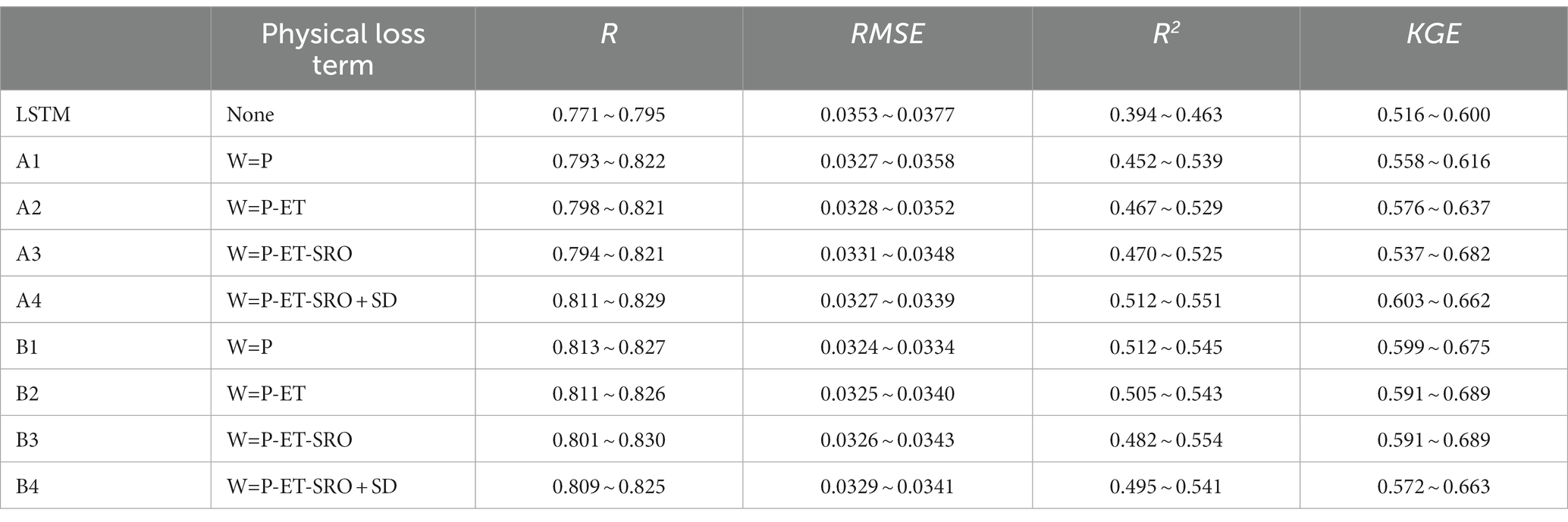
Table 1. Impact of different loss functions on LSTM models.

In summary, LSTM models employing the water balance loss function outperform traditional models in several aspects, including lower root mean square error (RMSE), higher linear correlation (R, R²), and improved simulation and prediction performance (KGE). It may be more suitable for modeling and predicting the relationship between surface water and single-layer soil water, possibly due to the more coherent and direct physical connection between surface water and single-layer soil water. Surface water is typically directly influenced by factors like precipitation, evaporation, and surface runoff, which interact more directly with single-layer soil water. This direct interaction makes it easier for the model to capture the physical processes between surface water and soil water. Additionally, the relationship between surface water and single-layer soil water is relatively simple, resulting in lower predictive uncertainty. In contrast, multi-layer soil water systems may involve more unknown factors, leading to greater predictive uncertainty. This highlights the crucial role of appropriately designed loss functions and water balance formulas in improving model performance.

3.2 Investigation of weight impact on loss functions

The results in groups C and D are based on our study of weight adjustments. We chose to compare A4 (group C) and B4 (group D) for our analysis. Different experiments employed varying ratios of RMSE and physical loss weights, ranging from 1:9 to 9:1. These weight ratios determine the relative importance of RMSE and physical constraints during model training. A higher RMSE weight ratio places more emphasis on data fitting, while a higher PHY weight ratio signifies greater focus on fitting physical constraints (Table 2).

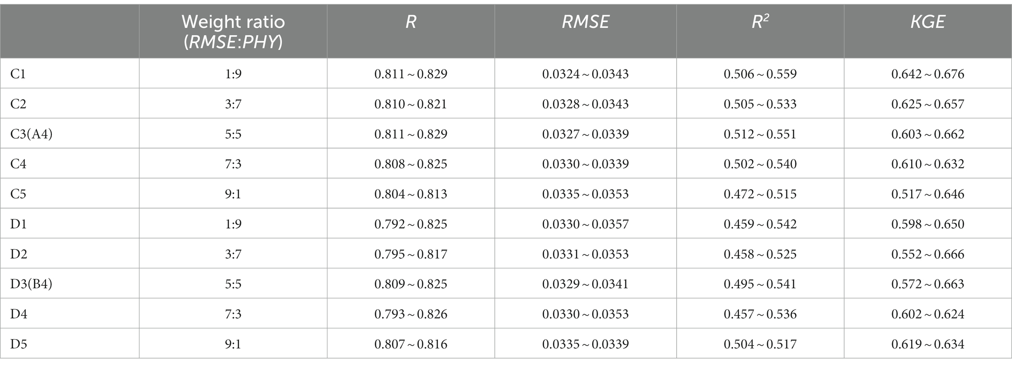
Table 2. Impact of different loss weights on LSTM models.

From the experimental results, we observed that different weight ratios significantly influenced the model’s predictive performance. In group C, C1 performed exceptionally well across all metrics, indicating its superior predictive capabilities. This is attributed to the 1:9 RMSE:PHY weight ratio, which places stronger emphasis on the influence of physical factors. Conversely, C5 exhibited relatively poor performance across all metrics, suggesting weaker predictive abilities, possibly due to an excessive emphasis on data fitting. C2 and C4’s performance may have been influenced by their relatively unbalanced weight ratios, failing to clearly emphasize one aspect, resulting in less outstanding performance in any specific area. C3, adopting a 5:5 RMSE:PHY weight ratio, performed moderately well across all metrics, demonstrating overall stable predictive capabilities without excelling in any specific aspect.

The situation in group D is largely similar to that of group C. However, we found that D3 performed exceptionally well across all aspects, showing relatively stable predictive abilities. The experimental results underscore the critical role of weight ratios in model performance. Different tasks and problems may require distinct weight ratios to balance data fitting and physical constraints. In practical applications, careful consideration is needed to select the appropriate weight ratios based on task requirements and the relative importance of data and physical constraints.

3.3 Influence of different climates on model performance

Examining Figure 3A, it is evident that the R of the PHYs-LSTM model are slightly lower than those of the LSTM model in equatorial regions. This may be due to the high precipitation in equatorial regions, which results in more infiltration processes and multi-layer soil moisture saturation, ultimately leading to a decrease in the model’s predictive performance. Conversely, the PHYs-LSTM model outperforms the LSTM model in arid and polar climate regions. This might be attributed to lower precipitation in these regions and a higher linear correlation between deep soil moisture and surface water, resulting in better performance by the PHYs-LSTM model in these areas. The PHY-LSTM model surpasses the LSTM model in all climate zones, with slight exceptions in some regions. This could be linked to higher linear correlation between surface soil moisture and surface water in well-watered areas, whereas in drier regions, the correlation between surface soil moisture and surface water is more dependent on changes in deep soil moisture.

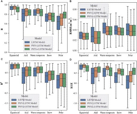
Figure 3. Boxplot of the performance of three deep learning models in predicting 1-day future outcomes in different climate regions. (A) the climate zone box plots showcase the R for each model. (B) displays box plots for the RMSE in different climate zones. (C) while illustrates the box plots for the R² values across these zones. Lastly, (D) depicts the KGE box plots for climate regions. The horizontal axis of each figure represents distinct climate zones, and the vertical axis signifies the corresponding metric values. Each box plot consists of five horizontal lines representing the maximum, 75th percentile, median, 25th percentile, and minimum values derived from the simulations of each deep learning model.

As shown in Figures 3B,C, the RMSE of PHYs-LSTM and PHY-LSTM models in various climate zones are quite close and lower than those of the LSTM model. This indicates that using physical loss functions (PHYs-LSTM and PHY-LSTM) to some extent helps the model fit observed data better and reduce prediction errors. R² of PHYs-LSTM and PHY-LSTM models in all climate zones are higher than those of the LSTM model, consistent with the RMSE. This suggests that physical loss functions contribute to improving the model’s explanatory power and better fitting the data trends.

The KGE of PHYs-LSTM and PHY-LSTM models outperform the LSTM model in most climate zones (Figure 3D), indicating that physical loss functions are better at capturing the consistency and relative errors in model performance. The lower performance of the PHYs-LSTM model in equatorial regions might be due to the high precipitation in that area. It may necessitate a reconsideration or redesign of the horizontal balance loss function for regions with prolonged rainfall.

In summary, the use of physical loss functions (PHYs-LSTM and PHY-LSTM) enhances model performance, especially in regions with different climate characteristics. These findings demonstrate that physical constraints can improve the model’s fit to observed data and its interpretability, but they also require appropriate adjustments and optimizations under varying geographic and climatic conditions. Different loss functions may require different parameter settings for optimal performance in different regions (see Table 1).

3.4 Physical consistency

Figure 4 illustrates the improvements in physical consistency for the PHYs-LSTM and PHY-LSTM models relative to the traditional LSTM model. Both the PHYs-LSTM and PHY-LSTM models demonstrate positive improvements in physical consistency compared to the traditional LSTM model in most regions. This indicates that physical loss functions (PHY-LSTM and PHYs-LSTM) offer better fitting to observed data and account for physical constraints, further enhancing model performance in these areas. However, there is a decline in the effectiveness of these models in Western Europe, Northwestern India, and Eastern Australia. This might be associated with the unique climatic, geographical, and soil characteristics of these regions, which may require more model adjustments and physical constraints to achieve improved performance. These regions are influenced by monsoon climates, typically characterized by seasonal rainfall distribution with abundant summer rains and relatively dry winters. This climatic feature could significantly impact water resource management and soil moisture prediction. Despite experiencing substantial precipitation during monsoon seasons, these areas may have uneven rainfall distribution across regions, leading to variations in wet and dry seasons. The impact of this non-uniform rainfall distribution on soil moisture can vary by region.

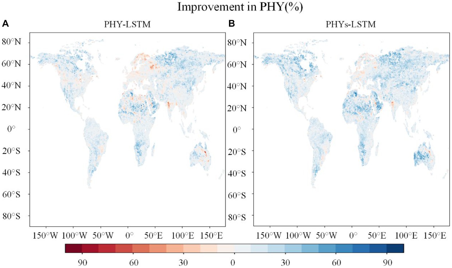
Figure 4. (A, B) Improvements in physical consistency achieved by LSTM models in predicting soil moisture 1 day into the future guided by physical knowledge. Both panels present improvement maps relative to traditional LSTM results. The vertical axis corresponds to latitude, the horizontal axis represents longitude, and the color scheme denotes the degree of improvement. Blue indicates enhancement, while red signifies no improvement. The intensity of the color reflects the extent of improvement or lack thereof.

In summary, variations in meteorological, soil, and geographical factors, as well as differences in data availability between regions, can lead to variations in prediction quality across regions. In each region, careful adjustment of model parameters and loss function weights is necessary to best adapt to specific geographical and meteorological conditions (see Table 2).

3.5 Time series plots

In Figure 5, it is evident that the prediction curves of the PHYs-LSTM and PHY-LSTM models, highlighted within the red circles, closely align with the observed data curves, especially when the soil moisture is not at saturation. This suggests that LSTM models incorporating physical constraints (PHYs-LSTM and PHY-LSTM) effectively capture changes in soil moisture, whether it is increasing or decreasing. This indicates the reasonableness of the designed balance loss function concerning soil moisture unsaturation, and it highlights a monotonic relationship between surface water variables and soil moisture during significant soil moisture fluctuations.

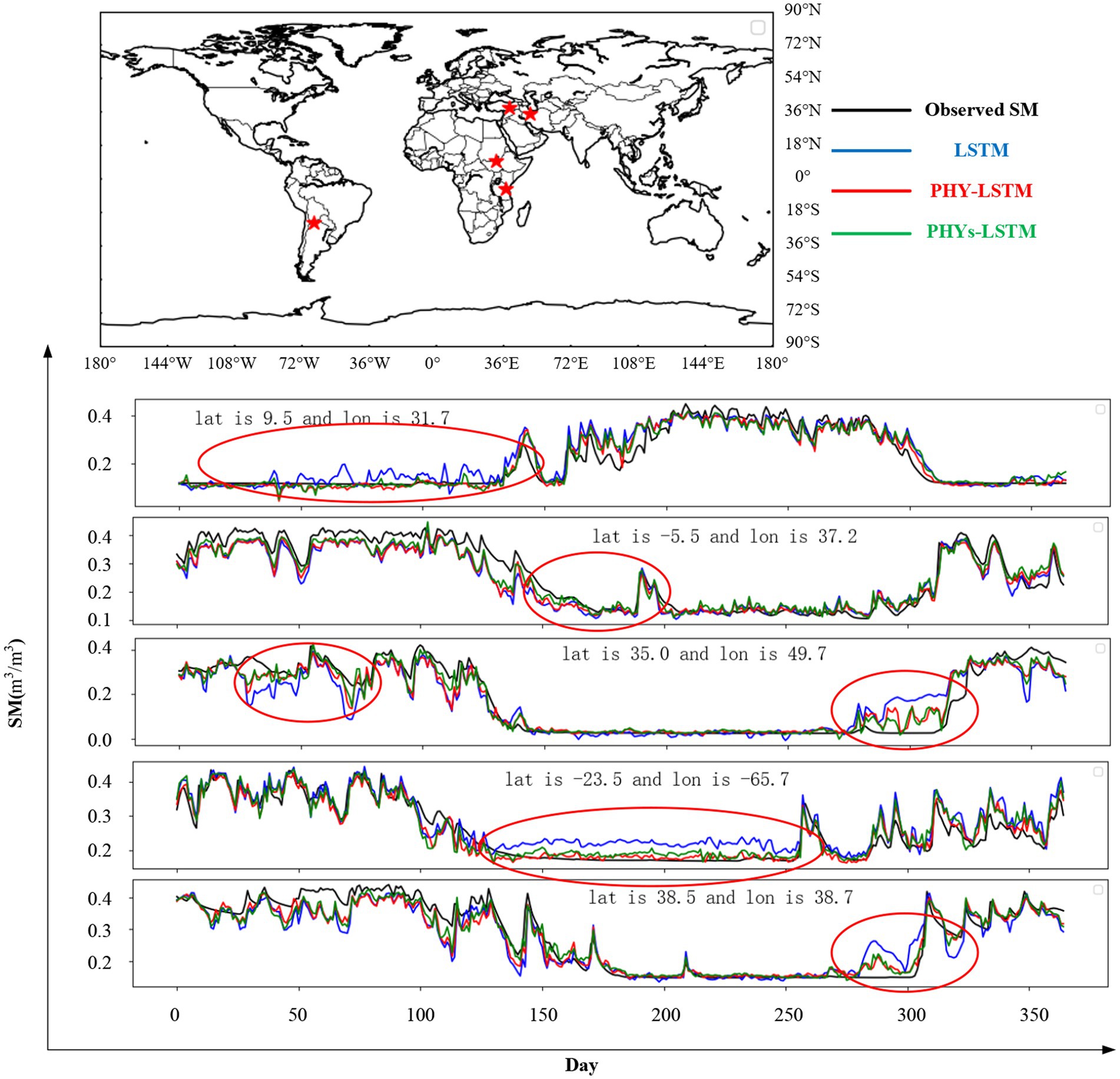
Figure 5. Time series plots for 1-day ahead predictions of 3 LSTM models in different regions.

Moreover, even during time periods when soil moisture remains relatively stable, the predictions of these two physical models surpass those of the LSTM model using RMSE as the loss function. This improvement could be attributed to the dynamic equilibrium that exists between surface water and soil moisture during these time periods. Models incorporating physical constraints perform better in simulating such dynamic equilibrium states.

These results emphasize that physically constrained models utilizing balance loss functions exhibit strong performance in simulating the relationship between soil moisture and surface water, particularly when soil moisture undergoes significant changes or remains in a dynamic equilibrium state. This provides a valuable tool for water resource management and soil moisture prediction.

4 Conclusion

This study conducted a comprehensive comparative analysis of LSTM models and two physically constrained models, PHYs-LSTM and PHY-LSTM. The analysis primarily focused on the influence of multiple factors on different soil moisture depths, the impact of weight ratios on loss terms, variations under different climatic conditions, and the models’ physical consistency. When confronted with multiple influencing factors, LSTM models incorporating balance loss functions (PHYs-LSTM and PHY-LSTM) outperformed traditional LSTM models. They exhibited lower Root Mean Square Error (RMSE), higher linear correlations (R, R²), and superior simulation and prediction performance (KGE). This demonstrates that balance loss functions contribute to reducing prediction errors and improving the alignment of the models with observed data. Weight ratios significantly influenced model performance. Appropriate weight ratios can balance data fitting and physical constraints to achieve optimal performance. Higher RMSE weight ratios emphasize data fitting, while higher physical constraint weight ratios emphasize the fitting of physical factors. Different tasks may require different weight ratios, depending on the relative importance of data and physical constraints.

PHYs-LSTM and PHY-LSTM models exhibited positive improvements relative to traditional LSTM models in most regions, highlighting the positive impact of physical loss functions on fitting observed data and considering physical constraints to further enhance model performance. However, in some regions, such as Western Europe, Northwest India, and Eastern Australia, the improvements were less pronounced, possibly due to the unique climatic, geographic, and soil characteristics in these areas. Future improvements may involve further optimization of loss functions and adjustments to weight ratios to better balance data fitting and physical constraints. For instance, region-specific loss functions could be designed, considering that each region may involve different surface water variables and soil moisture depths in their respective loss functions. Such customized differentiations have the potential to enhance model adaptability and performance.

Data availability statement

The original contributions presented in the study are included in the article/supplementary material, further inquiries can be directed to the corresponding author.

Author contributions

QG: Formal analysis, Funding acquisition, Resources, Supervision, Writing – review & editing. SY: Investigation, Methodology, Project administration, Software, Validation, Visualization, Writing – original draft, Writing – review & editing. QL: Conceptualization, Investigation, Writing – review & editing. CZ: Data curation, Software, Writing – review & editing.

Funding

The author(s) declare financial support was received for the research, authorship, and/or publication of this article. The study was partially supported by the National Natural Science Foundation of China, grant numbers 42275155, 42105144, 42205149 and U1811464, the Jilin Provincial Science and Technology Development Plan Project under grant 20230101370JC, and the Jilin Provincial Department of Education Science and Technology Research Project under grant JJKH20220840KJ.

Conflict of interest

The authors declare that the research was conducted in the absence of any commercial or financial relationships that could be construed as a potential conflict of interest.

Publisher’s note

All claims expressed in this article are solely those of the authors and do not necessarily represent those of their affiliated organizations, or those of the publisher, the editors and the reviewers. Any product that may be evaluated in this article, or claim that may be made by its manufacturer, is not guaranteed or endorsed by the publisher.

References

Beven, K. (2006). A manifesto for the equifinality thesis. J. Hydrol. 320, 18–36. doi: 10.1016/j.jhydrol.2005.07.007
Brocca, L., Ciabatta, L., Massari, C., Camici, S., and Tarpanelli, A. (2017). Soil moisture for hydrological applications: open questions and new opportunities. Water 9:140. doi: 10.3390/w9020140
Cai, Y., Zheng, W., Zhang, X., Zhangzhong, L., and Xue, X. (2019). Research on soil moisture prediction model based on deep learning. PLoS One 14:e0214508. doi: 10.1371/journal.pone.0214508
Chopart, J. L., and Vauclin, M. (1990). Water balance estimation model: field test and sensitivity analysis. Soil Sci. Soc. Am. J. 54, 1377–1384. doi: 10.2136/sssaj1990.03615995005400050029x
Cosgrove, B. A., Lohmann, D., Mitchell, K. E., Houser, P. R., Wood, E. F., Schaake, J. C., et al. (2003). Real-time and retrospective forcing in the north American land data assimilation system (NLDAS) project. J. Geophys. Res. Atmos. 108, 1887–1902. doi: 10.1029/2002JD003118
Diouf, D., Mejia, C., and Seck, D., (2020). Soil moisture prediction model from ERA5-land parameters using a deep neural networks. Proceedings of the 12th International Joint Conference on Computational Intelligence (IJCCI 2020), pp. 389–395.
Dueben, P. D., and Bauer, P. (2018). Challenges and design choices for global weather and climate models based on machine learning. Geosci. Model Dev. 11, 3999–4009. doi: 10.5194/gmd-11-3999-2018
Eltahir, E. A. B. (1998). A soil moisture-rainfall feedback mechanism: theory and observations. Water Resour. Res. 34, 765–776. doi: 10.1029/97WR03497
Fang, K., Pan, M., and Shen, C. (2019). The value of SMAP for long-term soil moisture estimation with the help of deep learning. IEEE Trans. Geosci. Remote Sens. 57, 2221–2233. doi: 10.1109/TGRS.2018.2872131
Fang, K., and Shen, C. (2020). Near-real-time forecast of satellite-based soil moisture using long short-term memory with an adaptive data integration Kerne. J. Hydrometeorol. 21, 399–413. doi: 10.1175/JHM-D-19-0169.1
Fang, K., Shen, C., Kifer, D., and Yang, X. (2017). Prolongation of SMAP to Spatio-temporally seamless coverage of continental US using a deep learning neural network. Geophys. Res. Lett. 44, 11,030–11,039. doi: 10.1002/2017GL072874
Feng, D., Fang, K., and Shen, C. (2020). Enhancing streamflow forecast and extracting insights using long-short term memory networks with data integration at continental scales. Water Resour. Res. 56. doi: 10.1029/2019WR026793
Friedl, M. A., Sulla-Menashe, D., Tan, B., Schneider, A., Ramankutty, N., Sibley, A., et al. (2010). MODIS collection 5 global land cover: algorithm refinements and characterization of new datasets. Remote Sens. Environ. 114, 168–182. doi: 10.1016/j.rse.2009.08.016
Henderson-Sellers, S. A. (1996). Validation of soil moisture simulation in landsurface parameterisation schemes with HAPEX data. Glob. Planet. Chang. 13, 11–46. doi: 10.1016/0921-8181(95)00038-0
Hochreiter, S., and Schmidhuber, J. (1997). Long short-term memory. Neural Comput. 9, 1735–1780. doi: 10.1162/neco.1997.9.8.1735
Jia, X., Willard, J., Karpatne, A., Read, J. S., Zwart, J. A., Steinbach, M., et al. (2021). Physics-guided machine learning for scientific discovery: an application in simulating Lake temperature profiles. ACM/IMS Trans. Data Sci. 2, 1–26. doi: 10.1145/3447814
Jia, X., Zwart, J., Sadler, J., Appling, A., and Kumar, V., (2020). Physics-guided recurrent graph networks for predicting flow and temperature in river networks. doi: 10.48550/arXiv.2009.12575
Kahana, A., Turkel, E., Dekel, S., and Givoli, D. (2020). Obstacle segmentation based on the wave equation and deep learning. J. Comput. Phys. 413:109458. doi: 10.1016/j.jcp.2020.109458
Karpatne, A., Watkins, W., Read, J., and Kumar, V., (2017). Physics-guided neural networks (PGNN): an application in Lake temperature modeling. doi: 10.48550/arXiv.1710.11431
Kroes, J. G., Wesseling, J. G., and Van, D. J. C. (2000). Integrated modelling of the soil-water-atmosphere-plant system using the model SWAP 2.0 an overview of theory and an application. Hydrol. Process. 14, 1993–2002. doi: 10.1002/1099-1085(20000815/30)14:11/123.0.CO;2-#
Lazer, D., Kennedy, R., King, G., and Vespignani, A. (2014). The parable of Google flu: traps in big data analysis. Science 343, 1203–1205. doi: 10.1126/science.1248506
Li, Q., Li, Z., Shangguan, W., Wang, X., Li, L., and Yu, F. (2022a). Improving soil moisture prediction using a novel encoder-decoder model with residual learning. Comput. Electron. Agric. 195:106816. doi: 10.1016/j.compag.2022.106816
Li, Q., Wang, Z., Shangguan, W., Li, L., Yao, Y., and Yu, F. (2021). Improved daily SMAP satellite soil moisture prediction over China using deep learning model with transfer learning. J. Hydrol. 600:126698. doi: 10.1016/j.jhydrol.2021.126698
Li, Q., Zhang, C., Shangguan, W., Li, L., and Dai, Y. (2023). A novel local-global dependency deep learning model for soil mapping. Geoderma 438:116649. doi: 10.1016/j.geoderma.2023.116649
Li, Q., Zhang, C., Shangguan, W., Wei, Z., Yuan, H., Zhu, J., et al. (2024). LandBench 1.0: a benchmark dataset and evaluation metrics for data-driven land surface variables prediction. Expert Syst. Appl. 243:122917. doi: 10.1016/j.eswa.2023.122917
Li, Q., Zhu, Y., Shangguan, W., Wang, X., Li, L., and Yu, F. (2022b). An attention-aware LSTM model for soil moisture and soil temperature prediction. Geoderma 409:115651. doi: 10.1016/j.geoderma.2021.115651
Luo, P., Song, Y., Huang, X., Ma, H., Liu, J., Yao, Y., et al. (2022). Identifying determinants of spatio-temporal disparities in soil moisture of the northern hemisphere using a geographically optimal zones-based heterogeneity model. ISPRS J. Photogramm. Remote Sens. 185, 111–128. doi: 10.1016/j.isprsjprs.2022.01.009
Penman, L. H. (1948). Natural evaporation from open water, bare soil and grass. Proc. R. Soc. Lond. 193, 120–145. doi: 10.1098/rspa.1948.0037
Read, J. S., Oliver, S. K., Watkins, W., Jia, X., Willard, J., Appling, A. P., et al. (2019). Process-guided deep learning predictions of Lake water temperature. Water Resour. Res. 55, 9173–9190. doi: 10.1029/2019WR024922
Rosenzweig, C., Iglesias, A., Yang, X. B., Epstein, P. R., and Chivian, E. (2001). Climate change and extreme weather events; implications for food production, plant diseases, and pests. Glob. Change Hum. Health 2, 90–104. doi: 10.1023/A:1015086831467
Seneviratne, S. I., Corti, T., Davin, E. L., Hirschi, M., Jaeger, E. B., Lehner, I., et al. (2010). Investigating soil moisture–climate interactions in a changing climate: a review. Earth-Sci. Rev. 99, 125–161. doi: 10.1016/j.earscirev.2010.02.004
Solomon, S., Qin, D., Manning, M., Chen, Z., Marquis, M., Averyt, K. B., et al. (2007). Climate change 2007: the physical science basis. Contribution of working group I to the fourth assessment report of the intergovernmental panel on climate change (IPCC). Comput. Geom. 18, 95–123. doi: 10.1016/S0925-7721(01)00003-7
Thober, S., Kumar, R., Sheffield, J., Mai, J., Fer, D. S., and Samaniego, L. (2015). Seasonal soil moisture drought prediction over Europe using the north American multi-model ensemble (NMME). J. Hydrometeorol. 16, 2329–2344. doi: 10.1175/JHM-D-15-0053.1
Thornthwaite, C. W. (1948). An approach toward a rational classification of climate. Geogr. Rev. 38, 55–94. doi: 10.2307/210739
Walker, J. P., Willgoose, G. R., and Kalma, J. D. (2009). One-dimensional soil moisture profile retrieval by assimilation of near-surface measurements: a simplified soil moisture model and field application. J. Hydrometeorol. 2:356. doi: 10.1175/1525-7541(2001)0022.0.CO;2
Willard, J., Jia, X., Xu, S., Steinbach, M., and Kumar, V. (2022). Integrating scientific knowledge with machine learning for engineering and environmental systems. ACM Comput. Surv. 55, 1–37. doi: 10.1145/3514228
Xie, K., Liu, P., Xia, Q., Li, X., Liu, W., Zhang, X., et al. (2022). Global soil moisture storage capacity at 0.5° resolution for geoscientific modelling. J. Hydrol. 320:18–36. doi: 10.5194/essd-2022-217
Xie, K., Liu, P., Zhang, J., Han, D., Wang, G., and Shen, C. (2021). Physics-guided deep learning for rainfall-runoff modeling by considering extreme events and monotonic relationships. J. Hydrol. 603:127043. doi: 10.1016/j.jhydrol.2021.127043
Yamazaki, D., Ikeshima, D., Tawatari, R., Yamaguchi, T., O'Loughlin, F., Neal, J. C., et al. (2017). A high-accuracy map of global terrain elevations. Geophys. Res. Lett. 44, 5844–5853. doi: 10.1002/2017gl072874
Ying, K., Zhao, T., Zheng, X., Quan, X. W., Frederiksen, C. S., and Li, M. (2016). Predictable signals in seasonal mean soil moisture simulated with observation-based atmospheric forcing over China. Clim. Dyn. 47, 2373–2395. doi: 10.1007/s00382-015-2969-3
Keywords: deep learning, soil moisture, loss functions, water balance, physical mechanism
Citation: Geng Q, Yan S, Li Q and Zhang C (2024) Enhancing data-driven soil moisture modeling with physically-guided LSTM networks. Front. For. Glob. Change. 7:1353011. doi: 10.3389/ffgc.2024.1353011
Edited by:
Luca Brocca, National Research Council (CNR), ItalyReviewed by:
Fubo Zhao, Xi'an Jiaotong University, ChinaAnurag Vidyarthi, Graphic Era University, India
Copyright © 2024 Geng, Yan, Li and Zhang. This is an open-access article distributed under the terms of the Creative Commons Attribution License (CC BY). The use, distribution or reproduction in other forums is permitted, provided the original author(s) and the copyright owner(s) are credited and that the original publication in this journal is cited, in accordance with accepted academic practice. No use, distribution or reproduction is permitted which does not comply with these terms.
*Correspondence: Qingliang Li, liqingliang@ccsfu.edu.cn