Using enhanced vegetation index and land surface temperature to reconstruct the solar-induced chlorophyll fluorescence of forests and grasslands across latitude and phenology

1. Introduction

Forests and grasslands, being the major carbon-collecting terrestrial ecosystems worldwide, play key roles in regulating the global carbon cycle (Yao et al., 2022). Solar-induced chlorophyll fluorescence (SIF) is closely linked to plant photosynthetic rate and plant physiological state (Guanter et al., 2012). Effectively monitoring the SIF in forests and grasslands helps in evaluating their photosynthetic intensity and capacity to collect carbon. Some satellites provide SIF data retrieved from vegetation spectral reflectance. For example, the Orbiting Carbon Observation-2 (OCO-2) satellite detects the discontinuous SIF soundings at a 1.25 km × 2.25 km scale on its orbits and revisits a given place every 16 days. Scanning Imaging Absorption Spectrometer for Atmospheric Charts on the Envisat satellite revisits the same location every 6 days and detects the global SIF at a scale of 30 km × 240 km. GOME-2 retrieves the global SIF with a spatial resolution of 0.5° and a revisitation cycle of 2 days. Finally, the Troposphere Global Monitoring Instrument on the Sentinel-5 precursor satellite monitors global SIF products at a 7 km × 3.5 km scale with a 1-day revisit interval (Frankenberg et al., 2011).

Given that these SIF retrievals directly obtained from satellite observations suffer from low spatial resolution, discontinuity, or low temporal resolution, attempts have been made to reconstruct SIF from relative factors [such as some vegetation indices and meteorological factors (MFs)]. Guo et al. (2020) used 0.05° MODIS normalized difference vegetation index (NDVI), enhanced vegetation index (EVI), leaf area index (LAI), fraction of absorbed photosynthetically active radiation (fAPAR), and photosynthetically active radiation (PAR) as predictors for reconstructing SIF, whose spatial resolution was 1 km and R² = 0.71. Similarly, Li and Xiao (2019) used EVI, PAR, vapor pressure deficit (VPD), and air temperature of 0.05° MODIS to build a global seasonal scale regression model with an R² = 0.79, extending the discontinuous OCO-2 detection to 0.05° global SIF. Bontempo et al. (2020) used the 0.05° MODIS-derived VIs, surface temperature, precipitation rate, soil moisture data, and surface reflectance, along with the rainfall rate and soil moisture product of the Tropical Rainfall Monitoring Mission (TRMM-TMPA), in a regional seasonal scale regression, thereby reconstructing the 0.5° GOME-2 SIF in northeastern Brazil to 0.05°, with an R² = 0.74. Gensheimer et al. (2022) used NDVI, EVI, near-infrared reflectance of vegetation (NIRv), kernel normalized difference vegetation index (kNDVI), MODIS bands, and solar zenith angle (SZA), as well as MFs, to construct a convolutional neural network (CNN), which they named SIFnet (monthly regression at global scale), for non-US regions spanning 2018–2021. Their study showed that SIFnet was able to increase the resolution of Troposphere Global Monitoring Instrument SIF by a factor of 10 with an R² and root mean square error (RMSE) of 0.92 and 0.17, respectively. Ma et al. (2020) collected data from February 2007 to May 2019 and used various stress factors, such as NDVI, reflectance, SZA, and air temperature, to assemble a random forest model (monthly regression at a global scale) to downscale SIF (Ma et al., 2020). Their results showed that the R² and RMSE could reach 0.74 and 0.28, respectively. Kang et al. (2022) collected data from October to December 2020 in Xinjiang, China, and used stress factors such as the FPAR, Sentinel-2 bands, and surface reflectance to build a two-step CNN model (monthly regression at regional scale) to downscale SIF, where the R² reached 0.85. Similarly, Duveiller et al. (2020) used NDVI, EVI, evapotranspiration (ET), and NIRv for SIF's downscaling (regional monthly regression) from the European Alps to the east of the Andes and even around the Great Lakes of Africa, obtaining R² values up to 0.80. In earlier work, Joiner et al. (2013) used monthly regression at a global scale to extend the coverage, obtaining a global 0.05° SIF product based on 0.05° MODIS NDVI, surface reflectance, atmospheric absorption, and fluorescence radiance, where model R² =0.73.

In sum, these studies demonstrate that SIF reconstructions can be improved by including auxiliary vegetation indices (VIs) and MFs; however, challenges still remain. Some predictors have a relatively low space resolution, and their observations are not always accessible (e.g., PAR, FPAR, and MFs). In contrast, most of the vegetation indices are relatively accessible and reliable, and most vegetation index products have global coverage. Therefore, we selected EVI or NDVI as the main predictors to characterize vegetation conditions, as their data are available at a spatial resolution of up to 30 m. Moreover, the above-cited studies did not consider the influence of different spatial and phenological phases during the SIF reconstruction. Correlation analysis of predictors and SIF at distinct growth stages of vegetation revealed the contribution of predictors varying across phenological phases. Hence, it is necessary to explore the potential of combining data suitable to specific growth stages to improve the performance of a SIF reconstruction model.

This study's prime objectives were to shed the dependence of the traditional SIF reconstruction model on many predictors that are not easily obtained and to explore the potential of different phenological phases and spatial locations augmenting the SIF reconstruction model's performance. To achieve these two objectives, remote sensing data and scientific material collected via a literature survey were used, and grassland and forest regions across low, mid, and high latitudes were chosen as representative ecosystems. In this study, we propose a data combination approach that considers locations and phenological phases and discuss a high-resolution SIF reconstruction solution.

2. Materials and methods

This study's strategy is illustrated in Figure 1. It included the following five steps: (1) A total of six forest and grassland regions were selected, and a dataset consisting of their 0.5° EVI, NDVI, and LST information resampled from 0.05° MODIS products and 0.5° GOME-2 SIF data was first established; the EVI and NDVI data were then used to assess their relation with SIF. The results suggested that the SIF was more related to EVI than NDVI, so EVI and LST were selected as the final predictors for estimating SIF. (2) The idea of a combined sampling approach was proposed considering the locations and growth stages of vegetation to explore the extent to which time and spatial coverage of sample spans could improve SIF regression models in particular regions at specific growth stages. Experiments were carried out using the above dataset to investigate which data combination method was most suitable for the six forest and grassland regions for their various phenological stages. Models for regressing SIF in forest and grassland regions were then established by applying the above methodology. Three data combinations were proposed in this study: monthly regression at a global scale, seasonal regression at a regional scale, and monthly regression at a regional scale. (3) Sentinel-3 EVI data and MODIS LST data were adopted to reconstruct the 500 m SIF using these three models. (4) Both 0.5° GOME-2 SIF and 0.05° GOSIF were then employed to evaluate the reconstructed SIF. (5) Finally, the degree of correlation between GPP and SIF was assessed. Comparing the reconstituted SIF with GPP (gross primary productivity) illustrated the potential of the reconstituted SIF for estimating gross carbon fluxes (Gao et al., 2021; Pierrat et al., 2022).

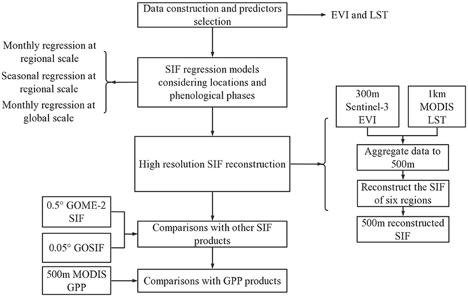
Figure 1. Framework for SIF reconstructions.

2.1. Study area

Six forest and grassland regions, located at low-, mid-, and high-latitude ranges, were selected as follows: The low-latitude forest (LLF; 0°-6°N, 9°-29°E) was near the border of Central Africa and Congo in Africa, where a tropical rainforest climate prevails, with high temperature and rain throughout the year. The mid-latitude forest (MLF; 22°-34°N, 98°-121°E) was in the Qin-Ling region of China, with a subtropical monsoon climate, where the annual average temperature was 15–22°C, and summer (June-August) rainfall accounted for ~50% of yearly precipitation. The high-latitude forest (HLF; 57°-65°N, 36°-58°E) was located in the Kostroma region of Russia, having a sub-frigid coniferous climate and rainfall concentrated in the warm season (July-August). The low-latitude grassland (LLG; 2°-14°N, 22°-48 E) was in Sudan of Africa, with a tropical grassland climate and high temperatures throughout the year and an annual average temperature of ~25°C; here, rainfall was concentrated in June-September, with the other months constituting a long dry season. The mid-latitude grassland (MLG; 36°- 45°N, 105°-122°E) was near the border area between Inner and Outer Mongolia, characterized by a temperate monsoon climate, with high temperatures and rainy summers (July-September) and winters that were cold and dry. The high-latitude grassland (HLG; 45°-53°N, 49°-80°E) was North of Balkhash, where the climate was temperate continental, being hot and humid in summer (July-August), yet cold and dry in winter. The study area is shown in Figure 2.

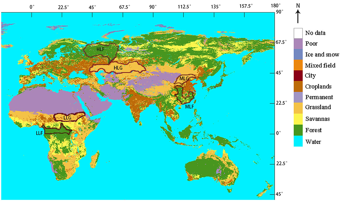
Figure 2. Six forest and grassland regions (areas enclosed by dark red lines). LLF (Low-latitude forest), MLF (Mid-latitude forest), HLF (High-latitude forest), LLG (Low-latitude grassland), MLG (Mid-latitude grassland), and HLG (High-latitude grassland). Land cover information was obtained from MODIS's MCD12C1.

2.2. Data collection

GOME-2 observes the global SIF at a spatial resolution of 0.5°. The spectral signal (650–800 nm) emitted by the photosynthetic center has two peaks of red light (~690 nm) and near-infrared (~740 nm), which can reflect strong fluorescent signals during peaks. We used the SIF values at 740 nm to evaluate the photosynthetic intensities of the six forest and grassland regions. The MODIS MOD13C2 and MOD11C3 data provided the global NDVI, EVI, and LST values once a month at a spatial resolution of 0.05°. As the spatial resolution of GOME-2 SIF data differs from that of MODIS, we first extracted the MODIS data points for the six forest and grassland regions and then aggregated them from 0.05° to 0.5°. For each GOME-2 SIF point with a latitude value of x and longitude value of y, those MODIS pointed within the latitudinal values of (x−0.025x + 0.025) and the longitudinal values of (y−0.025y + 0.025) were collected, to calculate their mean value, and this was used as the final matched value of that GOME-2 SIF point. Accordingly, a low-resolution dataset was generated, which contained the 0.5° GOME-2 SIF data for the six regions and their aggregated 0.5° NDVI, EVI, and LST values, to explore the quantitative relationships between SIF and its predictors.

In addition, Sentinel-3 images were geometrically corrected and cropped accordingly and then used to calculate the 300 m Sentinel-3 EVI values for the six regions using near red, red, and blue bands. Next, 300 m Sentinel-3 EVI data and 1 km MODIS LST from the six regions were resampled using ENVI to obtain the 500 m EVI information. For this resampling, the nearest-neighbor method was adopted to assign the nearest pixel value to the new pixel. Following this, MODIS MOD17A2H data were used to extract the 500 m GPP values for the six regions. Finally, a high-resolution dataset consisting of 500 m EVI, LST, and GPP values was obtained for the subsequent 500 m SIF reconstructions and validation, as shown in Table 1.

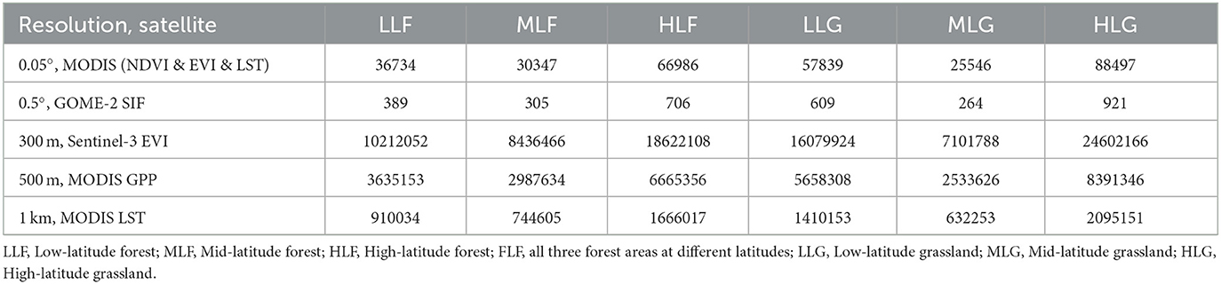
Table 1. Number of data points in the six forest and grassland regions.

2.2.1. SIF data

The global SIF data used in this study were provided by the NASA Aura Validation Data Center (http://avdc.gsfc.nasa.gov/) (Nechita and Chiriloaei, 2018). This consisted of far-red fluorescence (referenced wavelength: 740 nm) obtained from hyperspectral observations of the Global Ozone Monitoring Experiment-2 (GOME-2) instruments onboard the MetOp-A and MetOp-B satellites. We used the MetOp-A data from V28, whose daily observations are aggregated into monthly values, with cloud pollution reduced, resulting in a 0.5° level 3 product. Another SIF product obtained was GOSIF from the Global Ecology Group Data Repository (Li and Xiao, 2019), available from the https://globalecology.unh.edu/data/GOSIF.html.

2.2.2. MODIS data

The MODIS instrument, operating on the Terra and Aqua spacecraft, has a viewing swath width of 2330 km and views the entire surface of the Earth every 1 or 2 days. Three biophysical variables derived from the MODIS instrument were used to reconstruct the GOME-2 SIF in this study. The first two variables were NDVI and EVI, reflecting the green vegetation biomass on the planet's surface, being widely used in Earth monitoring. The reason for this is that NDVI and EVI, as commonly used vegetation indices, are freely available from many meter-level spatial resolution satellites. Both can be obtained from NASA's 0.05° MOD13C2 product and be computed using the following formulas:

where the EVI coefficients for MODIS are L = 1, C₁ = 5, C₂= 7.5, and G = 2.5 (Ma et al., 2020); ρ_NIR is the near-infrared band, ρ_RED is the red band, and ρ_BLUE is the blue band from the MODIS satellites.

The third variable was LST, the radiation temperature produced by the thermal infrared radiation emitted by the land surface. The LST of a given vegetation coverage area is mainly related to the canopy's top, representing the leaf layer having the highest photosynthetic rate. LST is also easier to obtain than other MFs, especially in some urban areas; it can be obtained from MOD11C3 with a 0.05° spatial resolution and MOD11A2 with a 1 km spatial resolution. To verify the reliability of the reconstructed SIF, we used the GPP product derived from MOD17A2H, for which one image is generated every 8 days with a spatial resolution of 500 m. Land use information came from the MCD12C1 product. All the above products can be downloaded from https://ladsweb.modaps.eosdis.nasa.gov/.

2.2.3. Sentinel-3 data

The Sentinel-3 satellite has two payloads: a Water Color Remote Sensing Instrument (OLCI) and a Sea Land Surface Temperature Radiometer (Zhang et al., 2020). OLCI is a push-broom imaging spectrometer that measures the solar radiation reflected by the Earth in 21 spectral bands with a ground-level spatial resolution of 300 m, spanning visible light to near-infrared (400–1020 nm). We used the full-resolution atmospheric radiation top product of OL_1_EFR in OLCI, with a revisitation period of 2 days and a spatial resolution of 300 m. That data product can be downloaded from https://scihub.copernicus.eu/dhus/#/home.

2.3. Variables selection

Light use efficiency (LUE) is a productivity model widely used to estimate GPP, net primary productivity, or crop yield in terrestrial ecosystems at different scales. According to LUE, we first identified explanatory variables that could explain SIF. Similar to the LUE approach for estimating GPP (Pei et al., 2022), SIF can be expressed as follows:

According to the above formula, SIF is proportional to the product of incoming PAR and fAPAR and the efficiency at which absorbed radiation is used in the photosynthesis process (ε_f). Therefore, we considered that vegetation conditions, meteorological conditions, and land cover information could be indispensable factors in predicting SIF. Considering which variables are easier to obtain for this factor, we used LST to characterize meteorological conditions because it can serve as a proxy of thermal stress in predictive models of SIF. Furthermore, we selected different dimensions as well as phenological phases of grassland and forest ecosystems as classification variables to develop the model, aiming to test whether a biome-specific model could improve the accuracy of SIF prediction. Finally, we prioritized EVI or NDVI to characterize vegetation conditions. To select the optimal explanatory variables, we compared the correlations of EVI and NDVI to SIF. Linear regression was applied to the low-resolution datasets in subsection 2.2, and the determined coefficient of determination (R²) and RMSE were used to compare the fit between SIF and its candidate predictors—NDVI and EVI. The above metrics were also used to evaluate the general performance of the SIF reconstruction model. Relative standard deviation (RSD) was used to measure the relative dispersion of data. Finally, the selected optimal predictor variables were applied for model development.

wherey_iis the true value, $\widehat{y}$_i is the predicted value, and $\bar{\mathit{y}}$ denotes the sample average; the term ${\displaystyle \sum _{i=1}^m}{({\widehat{y}}_i-y_i)}^2$ is the error caused by the predicted value, while the term${\displaystyle \sum _{i=1}^m}{(y_i-\bar{y})}^2$is the error caused by the sample average value; $\overline{x}$ is the mean of the sample, n is the total sample size, s is the sample variance, and x_i is a given sample's value.

2.4. Model development

The first step was to establish a linear regression model having the following regression equation:

where x₁ and x₂ are 0.5° EVI and 0.5° LST obtained in subsection 3.1 as the predictors, $\widehat{y}$ is 0.5° GOME-2 SIF as the predicted value, and a, b₁, and b₂ are undetermined parameters; using our generated dataset, the least-squares fitting method was applied to estimate those parameters and then bring them into the regression equation to obtain the prediction model.

The second step was to train the model. First, 75% of the samples were used as the training set (by default), setting aside the remaining 25% to serve as the testing set for the model. Then, using a 10-fold cross-validation method, the data were divided into 10 parts, one of which was designated as the validation set, and the others formed the training set. This was repeated 10 times. In this process, the hyper-parameters were kept constant, and their quality was gauged by the average training loss and average validation loss of the 10 model iterations. Finally, after obtaining a satisfactory hyper-parameter, we used all the data as the training set to obtain an optimal model.

3. Results

3.1. Variables' importance in the model

For forest regions in all three latitudes, relying solely on a greater spatial span did not perform well year-round (Figure 3A). Furthermore, the R² of SIF-EVI was higher than that of SIF-LST from April to August and November and exceeded that of SIF-NDVI from March to December. A similar pattern was found for low, mid, and HLGs, where the R² of SIF-EVI surpassed that of SIF-LST and SIF-NDVI in most months (Figures 3B–D).

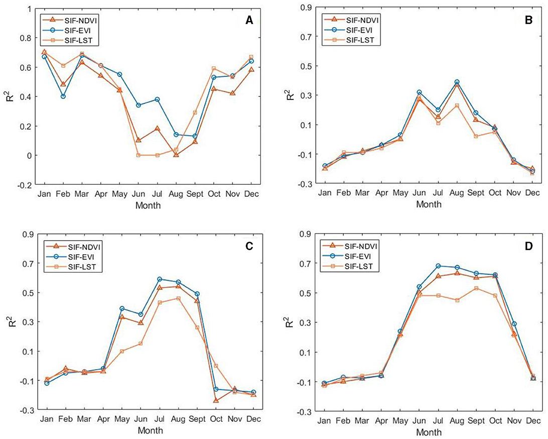
Figure 3. Comparison of correlations between SIF and candidate predictors EVI, NDVI, and LST. (A) Pooling forest regions across low, mid, and high latitudes. (B) High-latitude grassland region. (C) Mid-latitude grassland region. (D) Low-latitude grassland region.

The three factors of NDVI, EVI, and LST can yield four predictor combinations, including “NDVI&LST,” “EVI&LST,” “NDVI&EVI,” and “NDVI&EVI&LST.” Since “NDVI&EVI” was not representative, it is not discussed later as both are related to the photosynthesis of plants. The results showed that EVI and LST used in tandem could achieve the effect of combining all three factors, with the R² of EVI&LST-SIF outperforming that of NDVI&LST-SIF, with a smaller RMSE for EVI&LST-SIF (Figure 4). Therefore, the combination of EVI&LST was selected for the correlation experiment with SIF.

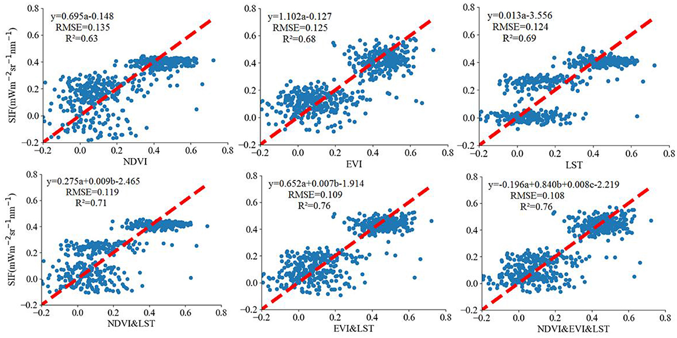
Figure 4. Results of SIF linear regressions from different combinations of NDVI, EVI, and LST in March in three forest regions. The coefficient “a,” “b,” and “c” of the regression equation in this study represents the variables on the horizontal axis.

3.2. Model performance over time and across latitude

First, to examine their temporal performance, we fit monthly linear regressions of SIF as a function of its EVI and LST predictors. These were derived by pooling all data from low-, mid-, and high-latitude forests. This showed that the monthly R² values from June to September were < 0.38, much lower than those in other months where the R² was between 0.55 and 0.76, as shown in Figure 5. Evidently, the mixed data of the three forest regions used for linear regression were not robust for all months of the year.

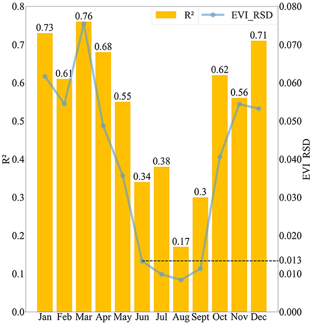
Figure 5. Comparison of the SIF regression models' performance with its predictor EVI's data dispersion. The numbers above the bars indicate the R² values of fitted SIF regression models in forest regions across low, mid, and high latitudes. The blue line indicates the relative standard deviation (RSD) of the EVI.

To investigate linear regression's poor performance from June to September, the following comparisons were made. Given that the EVI data were better correlated with SIF than the LST data (as mentioned in subsection 3.1), the dispersion of EVI data was examined to explain the variation in the SIF linear regression performance over time. The blue dots in Figure 5 show the extent to which the RSD of EVI data varies by month; clearly, the RSD values of EVI data decline steeply after March, bottoming out in August and then rising rapidly. Similar to the RSD of EVI data, the R² values of the SIF linear regression (yellow bars in Figure 5) also fell sharply from March, reached their lowest (worst) in August, and then rose rapidly. The variability of RSD values for EVI was basically consistent with that of the SIF linear regression's R².

The monthly EVI and LST data in June-September, though they came from all three regions corresponding to low-, mid-, and high-latitude forests, still had too narrow value ranges to produce satisfactory SIF regression models. Arguably, June to September is a crucial period for forests to capture carbon through intensive photosynthesis. In the following experiments, we tried to expand the value ranges of SIF and EVI by collecting data over a larger temporal span instead of a spatial span to bolster the linear regression performance. For the high-latitude forest region, the whole year can be divided into the following three stages: a dormant season (December-March), a growing season (April-July), and an aging season (August-November). Each growth stage entails 4 months, and all the 4-month SIF and its predictors' data were gathered together to fit linear regressions. Similarly, for the mid-latitude forest region, linear regressions were conducted on its dormant season (December-February), growing season (March-June), and aging season (July-November) separately. These results are presented in Table 2.

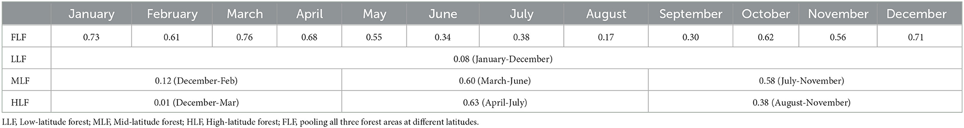
Table 2. The R² values of SIF regression models in forest regions.

For mid- and high-latitude forests, the R² values in their growing seasons (respectively, March-June and April-July) were 0.60 and 0.63, higher than that of either their dormant (mid-latitude forest: December-February, high-latitude forest: December-March) or aging seasons (mid-latitude forest: July-Noemberv, high-latitude forest: August-November). Figure 6 shows how R² and the RSD of EVI data vary over time in mid- and high-latitude forests. Similar to the results seen in Figure 5, a relatively wider value range of SIF and its predictor data could provide a better linear regression performance with a higher R² value. The RSD value of EVI data in the growing season was 0.055 for the high-latitude forest and 0.052 for the mid-latitude forest, both much higher than that of dormant and aging seasons (0.006 and 0.015, respectively) for the high-latitude forest, and likewise the 0.012 and 0.037 in dormant and aging seasons for the mid-latitude forest. Besides, in the growing season, the R² for the high-latitude forest (yellow bar) was 0.63, higher than the 0.60 for the mid-latitude forest (blue bar), whereas, in the dormant and aging seasons, the R² for the high-latitude forest (yellow bar) was 0.01 and 0.38, respectively, both lower than the corresponding 0.12 and 0.58 values for the mid-latitude forest (blue bar).

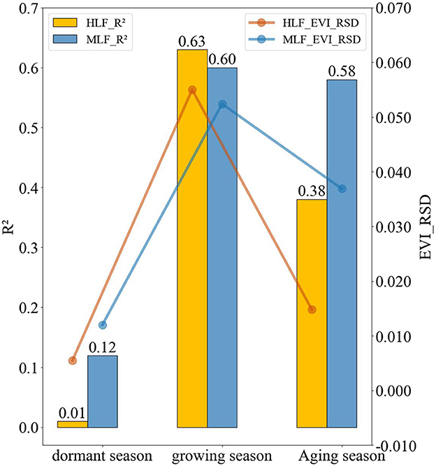
Figure 6. Comparison of the SIF regression models' performance and its predictor EVI's data dispersion in mid- and high-latitude forest regions at different phenological stages. The numbers above the bars indicate the R² values of fitted SIF regression models. The lines indicate the relative standard deviation (RSD) of the EVI data.

Linear regressions were also separately performed for the low-, mid-, and high-latitude grasslands. Table 3 presents their R² values on a monthly basis. Similar to the mid-latitude and high-latitude forests, the grasslands also had better SIF linear regression fits during the growing season but poorer ones during the other months. Specifically, although grass began to grow in the low-latitude region earlier than May, there was no significant increase in EVI due to their consumption by herbivory. From May onward, with a rising temperature and appropriate rainfall, grassland vegetation entered its rapid growth period, and the corresponding EVI values started to increase rapidly, generating relatively larger EVI disparities even within a single month; hence, the RSD of EVI data gradually increased from 0.015 to 0.061 in May to November, with the corresponding R² value improving from 0.22 to 0.65 during this period (Figure 7). A similar phenomenon was also observed in the mid- and high-latitude grassland regions, except that their growing periods were shorter than in the LLG region. Therefore, just like forests, the grasslands were also distinguished by a better SIF linear regression performance during their growing season than in other months. However, unlike forests, grasslands grew rapidly and could generate EVI data with large disparities even within a single month, so a large space or time span was not necessary for robust grassland SIF linear regressions. The following regressions were valuable for further SIF reconstructions: monthly regressions in June-October for low latitude, July-August for mid-latitude, and July for high latitude. Moreover, observations from both grassland and forest regions confirmed that using wider value ranges of EVI data could improve the SIF linear regressions.

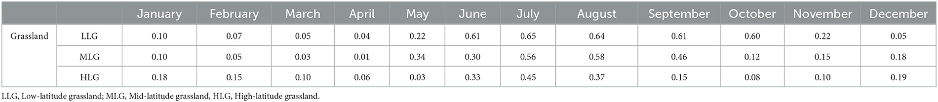
Table 3. The R² value of SIF regression models in grassland regions.

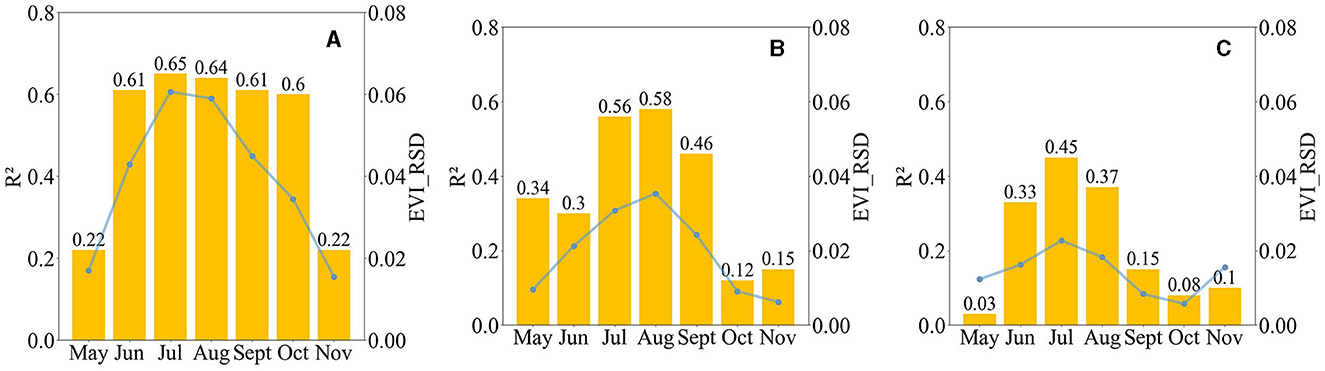
Figure 7. Comparison of the SIF regression models' performance and its predictor EVI's data dispersion in the grassland growing season (May-Nov). (A) In low-latitude grassland; (B) mid-latitude grassland; and (C) high-latitude grassland. The numbers above the bars indicate the R² values of fitted SIF regression models. The lines indicate the relative standard deviation (RSD) of the EVI data.

Overall, the following three data combinations were proposed in this study: monthly regression at a global scale, seasonal regression at a regional scale, and monthly regression at a regional scale (Table 4). For forests, data collected over large spatial spans provided adequate SIF linear regressions because tree leaves have completed their growth globally, but no significant differences were found in their EVI data during the intensive photosynthesis period from June through September (Figure 5; RSD of EVI was ≤0.013). Instead of the commonly used large-space span of global scales, we combined samples over an extended time span of growing seasons to amplify the disparities in EVI data. This revealed significantly improved R² values of SIF regression models in June-September for the mid-latitude forest region and in June-July for the high-latitude forest region. Therefore, the following regressions were valuable for the further reconstruction of SIF: Low-latitude forest from January to May, mid-latitude forest in January and February, and high-latitude forest from January to March, with all three forest regions from October to December recommended for conducting monthly SIF regression models based on EVI and LST at global scales. The mid-latitude forest in March-September and high-latitude forest in April-July were suitable for seasonal regression at regional scales, yet neither a large space nor time span could enhance the SIF regression models for the LLF in June-September and the high-latitude forest in August-September. The monthly regression at regional scales fit the LLG in June-October, the MLG in July-August, and the HLG in July.

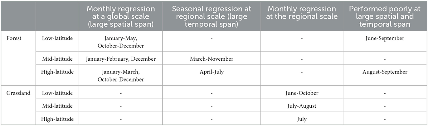
Table 4. Summary of sampling combination methods found suitable for forest and grassland regions.

3.3. Additional research on LLF

First, a relatively wider value range of SIF and its predictor data yielded a good SIF linear regression (as mentioned in subsection 3.2). However, the LLF had a much narrower range of SIF and EVI values, as evinced by Figure 8, which compared how SIF and EVI varied throughout the year. Unlike at mid or high latitudes, the LLF produced an annual EVI value within a much smaller range of variation (0.4~0.6). This was slightly lower in winter and spring and slightly higher in summer and autumn. RSD was used to evaluate the disparity in EVI and SIF data (Table 5). The RSD of EVI was 0.010 for LLF, much lower than 0.063 for the mid-latitude forest or 0.053 for the high-latitude forest. Similarly, the RSD of SIF was 0.037 in the low-latitude forest and likewise lower than 0.188 in the mid-latitude forest and 0.209 in the high-latitude forest.

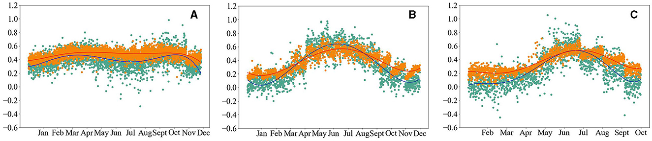
Figure 8. Variation in the EVI and SIF data across months in 2017. (A) Low-latitude forest. (B) Mid-latitude forest. (C) High-latitude forest. Green and orange scatter are the SIF and EVI data, with their fitted regressions curves in blue and red.

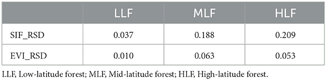
Table 5. The RSD values of SIF and EVI for LLF, MLF, and HLF.

3.4. Comparisons with other SIF products

We further compared the reconstructed SIF dataset with the results of 0.5° GOME-2 SIF and 0.05° GOSIF (Tables 6, 7). Regarding the comparison with GOME-2 SIF, we first aggregated the 500 m reconstructed SIF data to 0.5°. RMSE and R² were then used to evaluate the difference between the aggregate 0.5° SIF and 0.5° GOME-2 SIF data. Figures 9A–K shows the visual comparison of 0.5° GOME-2 SIF data and the 500 m reconstructed SIF data, which prove that the SIF images of forest and grassland have a finer spatial resolution after model reconstruction. The RMSE value of low-, mid-, and high-latitude grasslands was 0.097, 0.099, and 0.098, with an R² of 0.66, 0.51, and 0.62, respectively. For the mid-latitude forest, its RMSE values were 0.146 in March, 0.140 in April, and 0.152 in May; these were significantly better than the 0.446 in June, and the R² value for March-June was 0.70. The Sentinel-3 EVI data used to reconstruct SIF was more sensitive to clouds than the GOME-2 SIF data despite our efforts in searching for EVI images with lower cloud coverage. Specifically, the Sentinel-3 EVI data were more severely cloudy in June than in other months, as shown in the true-color images (Figure 10; the white portions are clouds). These clouds would block the satellite's field of view, seriously affecting their image acquisition and rendering the EVI in the blocked area invalid. The EVI index of bare ground tended to be zero, corresponding to the brown area in Figure 10A. However, due to the decoupling between SIF and EVI caused by other stress factors, the correlation between SIF and EVI was poor. The above two conditions seriously affected the reconstruction results of SIF. Accordingly, the RMSE between the reconstructed SIF data and GOME-2 SIF was significantly higher in June than in the other months. A similar phenomenon also occurred in the high-latitude forest, where RMSE values between the aggregated 0.5° SIF data and 0.5° GOME-2 SIF data were 0.178 in April, 0.167 in May, and 0.138 in July, all better than the 0.440 in June, which was clouded more than in other months, as shown in the true-color image (Figure 10; the white parts are clouds). Evidently, the proposed SIF reconstruction method, which considers a finer latitude differentiation and a reasonable time span and relies on only two predictors, EVI and LST, could provide reliable 500 m SIF. Nonetheless, this method was more sensitive to clouds than SIF satellite products due to its dependence on the vegetation index.

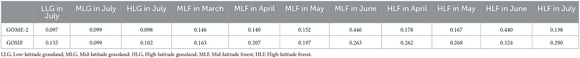
Table 6. The RMSE values between the reconstructed SIF and other SIF products.

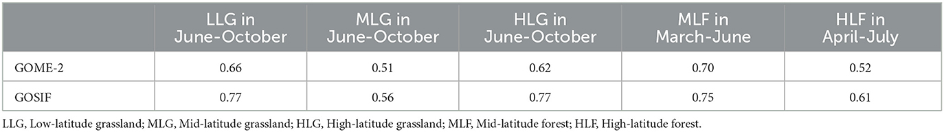
Table 7. The R² values between the reconstructed SIF and other SIF products.

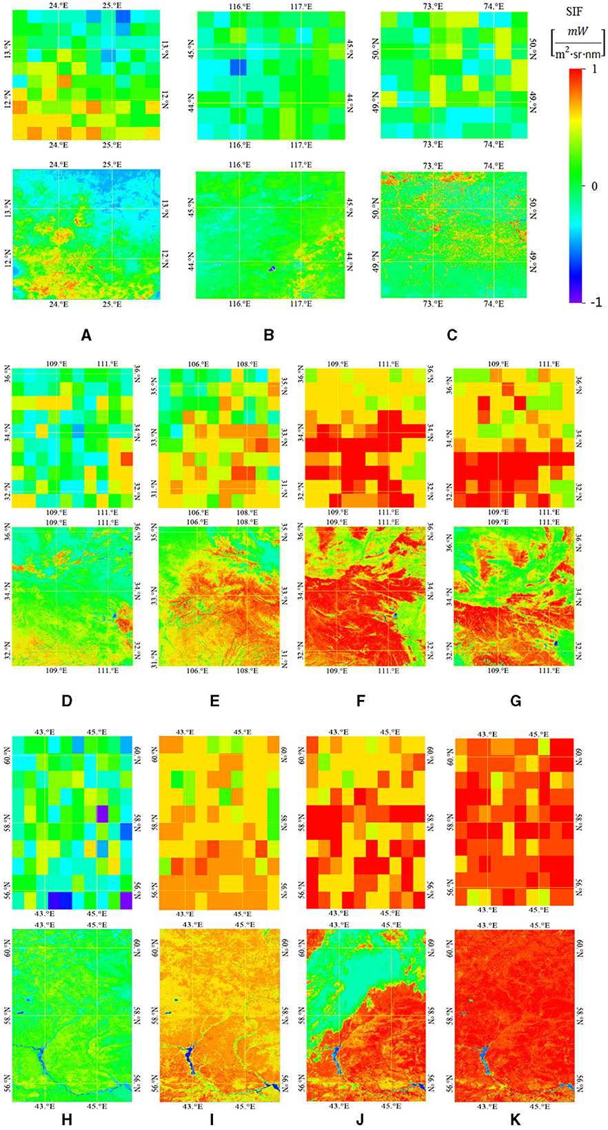
Figure 9. Comparisons of the 0.5° GOME-2 SIF and the 500 m reconstructed SIF in (A–K). (A) Low-latitude grassland in July. (B) Mid-latitude grassland in July. (C) High-latitude grassland in July. (D) Mid-latitude forest in March. (E) Mid-latitude forest in April. (F) Mid-latitude forest in May. (G) Mid-latitude forest in June. (H) High-latitude forest in April. (I) High-latitude forest in May. (J) High-latitude forest in June. (K) High-latitude forest in July.

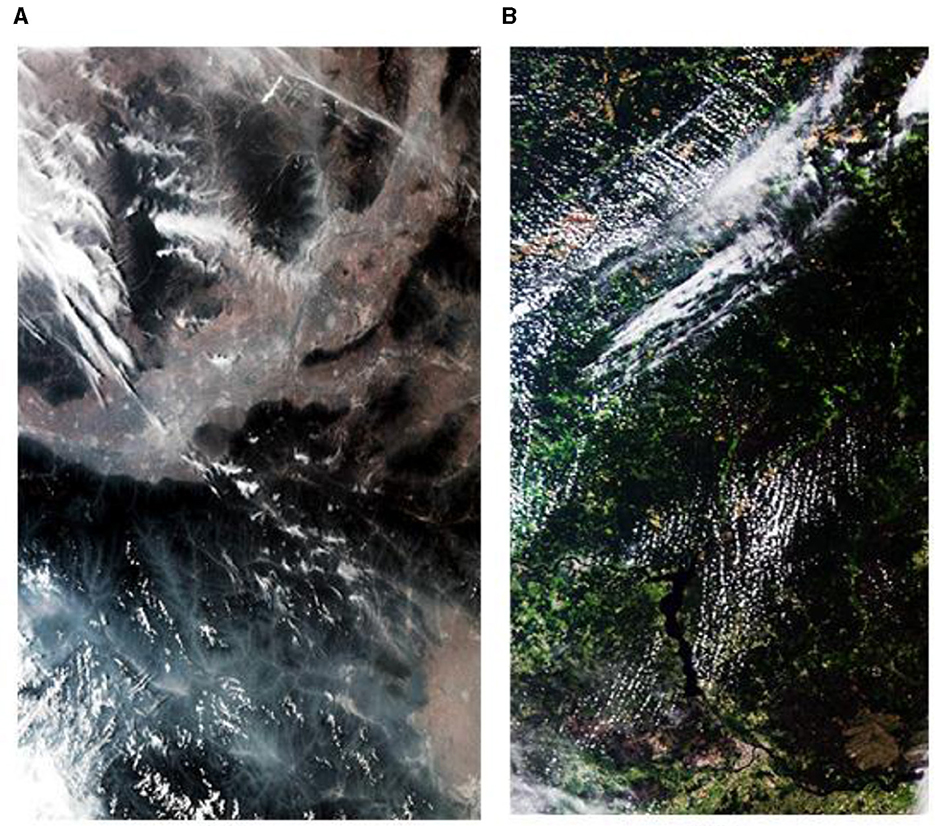
Figure 10. True-color Sentinel-3 EVI images of forest regions. (A) Mid-latitude forest in June 2017. (B) High-latitude forest in June 2017.

For the comparison with GOSIF, we obtained 2017 data from the GOSIF website at a spatial resolution of 0.05° and a temporal resolution of 1 month. The RMSE values fluctuated around 0.118 for grasslands and 0.246 for forests. The R² values reached 0.77 in both high- and low-latitude grassland regions in June-October and 0.75 in the mid-latitude forest region in March-June. Most of these GOSIF-based RMSE and R² values were slightly higher than those of GOME-2 SIF and the reconstructed SIF, and they did not work well when cloud cover was present, such as the high-latitude forests in June. Figures 11A–K shows the visual comparison of 0.05° GOSIF data and the 500 m reconstructed SIF data, which proved that the SIF images of forests and grasslands after undergoing model reconstruction had a high degree of similarity with those of GOSIF.

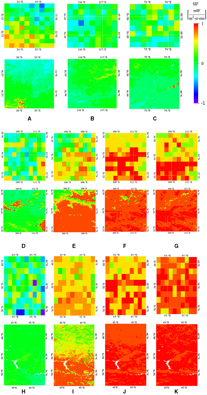
Figure 11. Comparisons of the 0.05° GOSIF and the 500 m reconstructed SIF in (A-K). (A) Low-latitude grassland in July. (B) Mid-latitude grassland in July. (C) High-latitude grassland in July. (D) Mid-latitude forest in March. (E) Mid-latitude forest in April. (F) Mid-latitude forest in May. (G) Mid-latitude forest in June. (H) High-latitude forest in April. (I) High-latitude forest in May. (J) High-latitude forest in June. (K) High-latitude forest in July.

3.5. Comparisons with GPP products

To further evaluate the reconstructed SIF product, we explored the relationship between it and GPP using the latter's estimates from the 500 m resolution MODIS. As Figure 12 shows, the reconstructed SIF product was closely related to GPP. The best R² of 0.97 appeared in the seasonal regression of mid-latitude grassland, and the lowest R² (0.90) came from the forest monthly regressions across low, mid, and high latitudes.

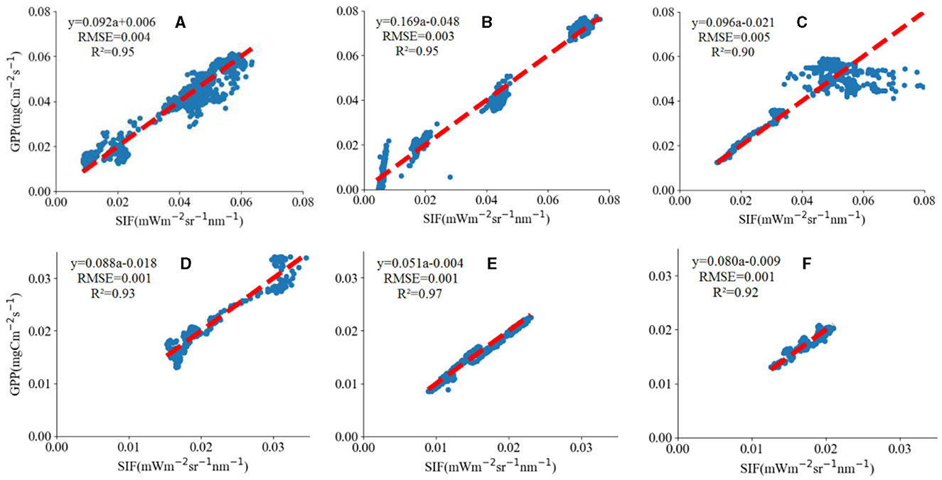
Figure 12. Correlations between the reconstructed SIF and GPP data. (A) Mid-latitude forest in Mar-Jun (B) High-latitude forest in Apr-Jul (C) All three forest regions across low, mid, and high latitude in Feb-Apr (D) Low-latitude grassland in July. (E) Mid-latitude grassland in July. (F) High-latitude grassland in July.

3.6. Interannual variations of coefficients in SIF model

Figure 13 compares the SIF model coefficients of 2017 and 2018. Pearson correlation coefficient (r) (eq. 8) was used to assess interannual variation in the SIF model coefficients, as follows:

where $\overline{x}$ and $\overline{y}$ represent the average value of a set of coefficients, x_i and y_i represent the coefficient value for each month separately. The results revealed that the EVI (LST) coefficients differ between years, even within the same month, especially during the summer. Nevertheless, the EVI (LST) coefficients still exhibited a high interannual correlation: the r was 0.744 for EVI coefficients and 0.820 for LST coefficients in forest regions. In contrast, significant interannual variation was detected in the grassland's EVI (LST) coefficients (Figure 13B), with r being −0.085 for EVI coefficients and 0.752 for LST coefficients. Grasslands were more sensitive to meteorological variation, herbivory (by vertebrates), and human interventions than forests.

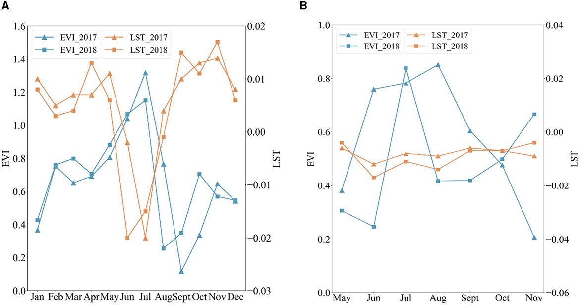
Figure 13. Variation in EVI and LST coefficients by month in the SIF regression models. (A) In forest regions across low, mid, and high latitudes. (B) Low-latitude grassland region. The red and blue lines represent EVI and LST, respectively, in both 2017 (circles) and 2018 (squares).

4. Discussion

4.1. Effects of EVI's RSD on model performance

EVI is less affected by the saturation effect than NDVI and performs better for forests and grasslands at certain stages of the growing season (Sun et al., 2020). For mixed forest areas at three latitudes, in most months of the year, the forests' phenology in low-, mid-, and high-latitude regions differed from each other, and their corresponding EVI also showed a pronounced discrepancy between latitudes and distribution within a wider range. Possible explanations for the changes in the RSD of EVI data are as follows: the high temperature at low latitudes allows its forest vegetation to grow vigorously, while the forests at mid-high latitudes must contend with a low-temperature environment and have few leaves, resulting in a large disparity of EVI values between the forests at low-latitude vs. mid-high latitudes. At mid-high latitudes, the temperature rises gradually from March, and the forests start to grow from then onward, forming dense stands in August; in tandem, their EVI values consequently increase, peaking in August, leading to the declining EVI disparity between the forests at low-latitude vs. mid-high latitudes from March until its trough in August. At mid-high latitudes, vegetation coverage gradually decreases from September onward as the temperature dips, while the LLF remains relatively dense due to the particularity of its tropical rainforest climate; hence, the EVI disparity between low-latitude forest vs. mid-high latitude forests rises again after September. Therefore, from June to September, because the tree leaves at all latitudes have basically completed growing, no obvious differences between latitudes in EVI data are discernable, and the EVI data at all latitudes are concentrated in a relatively smaller range, leading to a poor linear regression result. This explains why the R² values from June to September are lower.

For both mid- and high-latitude forests, the temperature and humidity in the growing season vis-à-vis the dormant or aging season are more suitable for vegetation growth—going from bare trees to those with dense leaves. Accordingly, the corresponding disparities of EVI values in the growing season exceed those of the other two seasons for both mid- and high-latitude forests. The latter has a subtropical coniferous forest climate where the warm period is shorter, and its precipitation falls only in the growing season, leading to green vegetation being sparse in the dormant and aging seasons (Nechita and Chiriloaei, 2018). In contrast, the mid-latitude forest has a subtropical monsoon climate with an annual average temperature of 15°C−22°C and abundant precipitation, so some vegetation coverage persists even during the dormant and aging season (Xia et al., 2019). As a result, the mid-latitude forest in the dominant and aging seasons provides EVI data with larger value ranges than the high-latitude region. Unlike the mid- and high-latitude regions, the low-latitude forest does not feature stark seasonal differences in terms of leaf areas index and photosynthetic intensity due to its tropical rainforest climate with high temperature and rainfall throughout the year (Leigh, 1975), leading to low EVI disparities over time and poor linear regressions of R² = 0.08 (please see subsection 3.2 for details). Therefore, the key to obtaining a sound and meaningful regression lies in using a relatively wider value range of EVI data. Consequently, it is recommended to collect the SIF and its predictors' data over a relatively larger spatial or temporal span to yield datasets with wider value ranges of SIF and its predictors for a more accurate SIF reconstruction.

4.2. Poor performance in LLF

There are two plausible explanations for the poor performance of linear regressions in the LLF region. This forest alone had a much narrower value range of SIF and EVI data, as seen in subsection 3.3. At mid-high latitudes, both SIF and EVI displayed an obvious seasonal cycle—they started to grow from March and peaked in summer given the favorable temperatures, soil moisture conditions, and longer sunshine hours, whereas in autumn (September, October, and November), SIF and EVI began to decline due to a drop in temperature and precipitation, reaching their lowest values in winter (December, January, and February). Unlike mid- or high-latitude regions, the forest at low-latitude produced an annual EVI value within a much smaller range of variation; it was slightly lower in winter and spring and slightly higher in summer and autumn. The RSD values for EVI and SIF were much lower for the LLF than for either the mid-latitude or high-latitude forest.

Another reason for the decoupling of SIF and EVI in LLF is that SIF, as a proxy of photosynthesis, is attributed to phenologically related structural changes (e.g., leaf abscission and leaf aging) as well as biochemical shifts in leaves (e.g., chlorophyll synthesis and degradation) (Chang et al., 2021), but EVI only depends on chlorophyll content, canopy structure, and green leaf area. The LLF region was mostly tropical rainforest with lush vegetation all year round and characterized by seasonal transitions between dry and wet. Under drought conditions—the dry season in the rainforest suggests a period of little, if any, rainfall—photosynthesis decreased in response to less light. On the contrary, the trees' deep roots kept absorbing groundwater during the dry season, enabling their EVI value to remain at a relatively high level, sustaining the lush vegetation of the tropical rainforest.

4.3. Comparisons with other relevant methods

Table 8 lists the predictors and model performance of past SIF-refactoring products. Comparatively, the model performance in this study reached a level on par with recent regional-scale SIF reconstruction products (Bontempo et al., 2020; Guo et al., 2020), i.e., our model R² for high and LLG regions reached 0.77 for the June-October period. In addition, we found that for the mid-latitude forest and HLG, their R² could be increased further when using a more complex algorithm. Compared with recent global-scale SIF reconstruction products (Li and Xiao, 2019; Ma et al., 2020; Gensheimer et al., 2022), the novelty of this study lies in not having to rely on predictors that are difficult to access, namely PAR, FPAR, and MFs. Only two predictors, EVI and LST, are required to reliably predict SIF, and it is easy to access the global rasterized high-spatial-resolution data for both (for instance, EVI data products have a spatial resolution of up to 30 m), enabling SIF to be predicted at a spatial resolution up to 10–100 m.

Table 8. Predictors and research scales used in previous SIF reconstruction studies (R²: coefficient of determination).

5. Conclusion

We proposed a simple method to reconstruct high-resolution SIF relying only on EVI and LST and explored the possibility of different phenological periods and spatial locations to augment the performance of SIF reconstruction models. Undoubtedly, high-resolution (e.g., 30 m) EVI information can now be freely acquired from many satellites, and temperature data are also widely and easily accessible, especially for human habitations. Our experiments show that the performance of SIF reconstruction models could be improved by further increasing the complexity of the algorithm. Our proposed method is, therefore, expected to be useful for reconstructing the SIF of forests and grasslands in and around urban and rural regions to help better evaluate the capacities of those vegetation ecosystems in collecting the carbon emitted by human activity.

Data availability statement

The raw data supporting the conclusions of this article will be made available by the authors, without undue reservation.

Author contributions

PZ: Conceptualization, Investigation, Methodology, Writing—original draft. HLiu: Writing—review and editing. HLi: Data curation, Writing—review and editing. JY: Software, Writing—review and editing. XC: Software, Writing—review and editing. JF: Formal analysis, Writing—review and editing.

Funding

The author(s) declare financial support was received for the research, authorship, and/or publication of this article. This study was supported by the Key Research and Development Plan of Anhui Province (Grant No. 2022l07020017), National Natural Science Foundation of China (Grant No. 61805001), and Natural Science Foundation of Anhui Province (Grant No. 1808085QF218).

Acknowledgments

We appreciate the research paper of Gregory Duveiller, which inspired this study.

Conflict of interest

The authors declare that the research was conducted in the absence of any commercial or financial relationships that could be construed as a potential conflict of interest.

Publisher's note

All claims expressed in this article are solely those of the authors and do not necessarily represent those of their affiliated organizations, or those of the publisher, the editors and the reviewers. Any product that may be evaluated in this article, or claim that may be made by its manufacturer, is not guaranteed or endorsed by the publisher.

References

Bontempo, E., Dalagnol, R., Ponzoni, F., and Valeriano, D. (2020). Adjustments to SIF aid the interpretation of drought responses at the Caatinga of Northeast Brazil. Remote Sens. 12, 3264. doi: 10.3390/rs12193264
Chang, C. Y., Wen, J., Han, J., Kira, O., LeVonne, J., Melkonian, J., et al. (2021). Unpacking the drivers of diurnal dynamics of sun-induced chlorophyll fluorescence (SIF): canopy structure, plant physiology, instruement configuration and retrieval methods. Remote Sens. Environ. 265, 112672. doi: 10.1016/j.rse.2021.112672
Duveiller, G., Filipponi, F., Walther, S., Köhler, P., Frankenberg, C., Guanter, L., et al. (2020). A spatially downscaled sun-induced fluorescence global product for enhanced monitoring of vegetation productivity. Earth Syst. Sci. Data 12, 1101–1116. doi: 10.5194/essd-12-1101-2020
Frankenberg, C., Fisher, J. B., Worden, J., Badgley, G., Saatchi, S. S., Lee, J. E., et al. (2011). New global observations of the terrestrial carbon cycle from GOSAT: patterns of plant fluorescence with gross primary productivity. Geophys. Res. Lett. 3, 1–14. doi: 10.1029/2011GL048738
Gao, H., Liu, S., Lu, W., Smith, A. R., Valbuena, R., Yan, W., et al. (2021). Global analysis of the relationship between reconstructed solar-induced chlorophyll fluorescence (SIF) and gross primary production (GPP). Remote Sens. 13, 2824. doi: 10.3390/rs13142824
Gensheimer, J., Turner, A. J., Köhler, P., Frankenberg, C., and Chen, J. (2022). A convolutional neural network for spatial downscaling of satellite-based solar-induced chlorophyll fluorescence (SIFnet). Biogeosciences 19, 1777–1793. doi: 10.5194/bg-19-1777-2022
Guanter, L., Frankenberg, C., Dudhia, A., Lewis, P. E., Gómez-Dans, J., Kuze, A., et al. (2012). Retrieval and global assessment of terrestrial chlorophyll fluorescence from GOSAT space measurements. Remote Sens. Environ. 121, 236–251. doi: 10.1016/j.rse.2012.02.006
Guo, M., Li, J., Huang, S., and Wen, L. (2020). Feasibility of using MODIS products to simulate sun-induced chlorophyll fluorescence (SIF) in boreal forests. Remote Sens. 12, 680. doi: 10.3390/rs12040680
Joiner, J., Guanter, L., Lindstrot, R., Voigt, M., Vasilkov, A., Middleton, E., et al. (2013). Global monitoring of terrestrial chlorophyll fluorescence from moderate spectral resolution near-infrared satellite measurements: methodology, simulations, and application to GOME-2. Atmos. Meas. Tech. Discuss. 6, 3883–3930. doi: 10.5194/amt-6-2803-2013
Kang, X., Huang, C., Zhang, L., Zhang, Z., and Lv, X. (2022). Down scaling solar-induced chlorophyll fluorescence for field-scale cotton yield estimation by a two-step convolutional neural network. Comput. Electron. Agric. 201, 107260. doi: 10.1016/j.compag.2022.107260
Leigh, E. G. (1975). Structure and climate in tropical rain forest. Ann. Rev. Ecol. Syst. 6, 67–86. doi: 10.1146/annurev.es.06.110175.000435
Li, X., and Xiao, J. (2019). A global, 0.05-degree product of solar-induced chlorophyll fluorescence derived from OCO-2, MODIS, and reanalysis data. Remote Sens. 11, 517. doi: 10.3390/rs11050517
Ma, Y., Liu, L., Chen, R., Du, S., and Liu, X. (2020). Generation of a global spatially continuous TanSat solar-induced chlorophyll fluorescence product by considering the impact of the solar radiation intensity. Remote Sens. 12, 2167. doi: 10.3390/rs12132167
Nechita, C., and Chiriloaei, F. (2018). Interpreting the effect of regional climate fluctuations on Quercus robur L. trees under a temperate continental climate (southern Romania). Dendrobiology 12, 77–89. doi: 10.12657/denbio.079.007
Pei, Y., Dong, J., Zhang, Y., Yuan, W., Doughty, R., Yang, J., et al. (2022). Evolution of light use efficiency models: improvement, uncertainties, and implications. Agric. Forest Meteorol. 317, 108905. doi: 10.1016/j.agrformet.2022.108905
Pierrat, Z., Magney, T., Parazoo, N. C., Grossmann, K., Bowling, D. R., Seibt, U., et al. (2022). Diurnal and seasonal dynamics of solar-induced chlorophyll fluorescence, vegetation indices, and gross primary productivity in the boreal forest. JGR Biogeosci. 127, e2021JG006588. doi: 10.1029/2021JG006588
Sun, X., Wang, M., Li, G., Wang, J., and Fan, Z. (2020). Divergent sensitivities of spaceborne solar-induced chlorophyll fluorescence to drought among different seasons and regions. ISPRS Int. J. Geo-Inf. 9, 542. doi: 10.3390/ijgi9090542
Xia, C., Chen, K., Zhou, J., Mei, J., Liu, Y., Liu, G., et al. (2019). Comparison of precipitation stable isotopes during wet and dry seasons in a subtropical monsoon climate region of China. Appl. Ecol. Environ. Res. 17, 11979–11993. doi: 10.15666/aeer/1705_1197911993
Yao, L., Liu, Y., Yang, D., Cai, Z., Wang, J., Lin, C., et al. (2022). Retrieval of solar-induced chlorophyll fluorescence (SIF) from satellite measurements: comparison of SIF between TanSat and OCO-2. Atmos. Meas. Tech. 15, 2125–2137. doi: 10.5194/amt-15-2125-2022
Keywords: GPP, SIF, EVI, MODIS, Sentinel-3
Citation: Zhang P, Liu H, Li H, Yao J, Chen X and Feng J (2023) Using enhanced vegetation index and land surface temperature to reconstruct the solar-induced chlorophyll fluorescence of forests and grasslands across latitude and phenology. Front. For. Glob. Change 6:1257287. doi: 10.3389/ffgc.2023.1257287
Received: 12 July 2023; Accepted: 21 September 2023;
Published: 20 October 2023.
Edited by:
Mohammad Ibrahim Khalil, University College Dublin, IrelandReviewed by:
Subhanil Guha, National Institute of Technology Raipur, IndiaMuhsan Ehsan, Bahria University, Pakistan
Copyright © 2023 Zhang, Liu, Li, Yao, Chen and Feng. This is an open-access article distributed under the terms of the Creative Commons Attribution License (CC BY). The use, distribution or reproduction in other forums is permitted, provided the original author(s) and the copyright owner(s) are credited and that the original publication in this journal is cited, in accordance with accepted academic practice. No use, distribution or reproduction is permitted which does not comply with these terms.
*Correspondence: Haiqiu Liu, hqliu2018@hotmail.com