A maximum entropy approach to defining geographic bounds on growth and yield model usage
 W. Spencer Peay
 Bronson P. Bullock
  Cristian R. Montes
- Plantation Management Research Cooperative, Warnell School of Forestry and Natural Resources, University of Georgia, Athens, GA, United States
Growth and yield models are essential tools in modern forestry, especially for intensively managed loblolly pine plantations in the southeastern United States. While model developers often have a good idea of where these models should be used with respect to geographic location, determining geographic bounds for model usage can be daunting. Such bounds provide suitable areas where model predictions are likely to behave as expected or identify areas where models may do a poor job of characterizing the growth of a resource. In this research, we adapted a niche model methodology, commonly used to identify suitable spots for species occurrence (maximum entropy), to identify areas for using growth and yield models built from plots established in the Lower Coastal Plain and Piedmont/Upper Coastal Plain in the southeastern United States. The results from this analysis identify areas with similar climatic envelopes and soil properties to the areas where data was collected to fit these growth and yield models. These areas show notable overlap with the areas prescribed for use by the evaluated growth and yield models and support practitioners use of these models throughout these regions. Furthermore, this methodology can be applied to different forest models built using large regional extents as long as climatic and soil values are available for each site.
1. Introduction
Growth and yield models are used as a tool for forest management to estimate future conditions of a given stand based on current and/or past information. When coupled with a cost structure, they are an essential tool for forest management in the southeastern United States (Weiskittel et al., 2011; Burkhart and Tomé, 2012; Burkhart et al., 2019) and elsewhere around the world. These models are developed for a wide array of end users, and each model system may have several different applications based on its intended use. Despite the sometimes vast differences among models, all growth and yield models are similar in that they contain some level of prediction uncertainty. This uncertainty stems from various factors, some of which are related to the data used to fit a model and the local climate or biophysical variables where this data was collected. These factors, sometimes referred to as physiographic or climatic measures (Weiskittel et al., 2011), include variables such as temperature, precipitation, vapor pressure deficit, slope, aspect, nutrient availability, and water availability. Each of these measures, along with many others, can affect the productivity of a forested site (Sampson and Allen, 1999; Coble et al., 2001; Jokela et al., 2004; Weiskittel et al., 2011; Restrepo et al., 2019). However, the mechanisms and the degree to which such factors affect productivity may differ for various sites, species, and regions.
Despite the correlation between productivity and some of the previously listed physiographic, climatic, and edaphic factors, they can be hard to include in a growth and yield system. A major difficulty is to collect or estimate such variables for each plot included in a modeling effort (Weiskittel et al., 2011), and depending on the scale or resolution of the model, it can be computationally inefficient to include such information. One approach model developers can elect to implement is dividing data into differing physiographic regions where these factors are similar; they can then fit different parameters or equations to each region. Examples of this approach are numerous, especially for loblolly pine plantations in the southeastern United States where distinctions are often made between the Piedmont and Coastal Plain physiographic regions (Harrison and Borders, 1996; Borders et al., 2004, 2014; Burkhart et al., 2008; ForesTech International LLC, 2009). When this approach is taken, developers often recommend a model be used in that particular region but make no statement as to whether a model can be applied throughout the entire region with similar levels of uncertainty or the uncertainty associated with using the model outside of a particular region. Thus, it is desirable to determine geographic bounds on growth and yield model usage. A similar problem is faced in species distribution modeling, range mapping, and similar disciplines where presence only and/or presence/absence data can be used in conjunction with some of the biophysical factors mentioned above to estimate the overall range of a species or its probability of occurrence in a particular area using several different techniques (Elith and Leathwick, 2009; Evans et al., 2016).
The past 20–30 years have seen dramatic changes in the modeling of species geographic distributions with the refining of traditional techniques and the application of newer techniques applied from a myriad of fields (Elith and Leathwick, 2009; Elith et al., 2011). One such development has been the use of maximum entropy modeling, a general-purpose machine learning technique that can help researchers to generate predictions or draw inferences from incomplete information such as presence-only data (Phillips et al., 2006; Elith et al., 2011). This approach works by estimating a probability distribution with the highest level of uncertainty, or in essence, estimates the probability distribution that makes the least amount of assumptions about the data and the probability of an event occurring while still satisfying a given set of constraints. One of the most popular tools for maximum entropy modeling is the MaxEnt framework implemented in Phillips et al. (2018). Over the past decade, this software has been commonly used in ecological and wildlife research to model geographic distributions and species' ranges or niche environments (Phillips and Dudík, 2008; Baldwin, 2009; Elith et al., 2011; Merow et al., 2013; Yang et al., 2013). This software has become popular partly due to its ease of use and predictive accuracy (Merow et al., 2013). Despite its use in these similar fields, MaxEnt has seen little use in forestry outside of the typical use to model the spatial distributions of tree species (Kumar and Stohlgren, 2009; Weber, 2011; Yang et al., 2013; Pollock, 2015; Qin et al., 2017).
This research focuses on a novel extension of MaxEnt to determine the geographic bounds of a growth and yield model. The model used to illustrate the methodology corresponds to one developed by the Plantation Management Research Cooperative (PMRC) at the University of Georgia. Using known geographic plot locations, biophysical factors such as temperature, precipitation, and soil properties were used as inputs to describe the niche that populations were growing into. These points and the biophysical data become the “species” of interest. The “probability of occurrence” now offers a pseudo-measure of suitability or uncertainty associated with using this particular growth and yield model in any given area within the study range. This measure of uncertainty is based on the differences in the environmental envelope between an area in question and the areas where data was collected to fit the PMRC 2014 growth and yield model (Borders et al., 2014). Determining suitable areas for model application is important to both model developers and users. It can allow parties to tailor model usage to specific geographic areas where a model may produce the most reliable estimates. Alternatively, identifying areas where a maximum entropy model suggests higher uncertainty levels can help inform developers, users, and forest resource managers where sampling efforts should be concentrated or increased to reduce this uncertainty in future model development.
2. Methods
2.1. Background
2.1.1. Maximum entropy principle
As mentioned previously, maximum entropy modeling uses machine learning algorithms to generate predictions or draw inferences from incomplete information (Phillips et al., 2006, 2017) and is based on the Maximum Entropy Principle first proffered by Jaynes (1957). This principle builds on Laplace's “Principle of Insufficient Reason,” an attempt to define the probability of two or more events based on little to no information. Laplace suggested that equal probabilities be assigned to two events if there is no evidence to think otherwise. The Maximum Entropy Principle builds on the Principle of Insufficient Reason where the probability distribution is derived as the distribution of maximum entropy and is thus only constrained by the supplied information; it is otherwise unaffected by missing information. The full derivation of the entropy of a probability distribution is presented in Jaynes (1957).
2.1.2. MaxEnt application to the proposed problem and associated assumptions
While this proposed use of MaxEnt is seemingly non-traditional, making several essential assumptions reduces the growth and yield model application problem to one that is similar to those currently implementing MaxEnt to model species' distributions. In our case, we assume the locations where data was collected to fit the PMRC 2014 growth and yield model are similar to the recorded presence of a species of interest in other applications. Absences, in this sense, are very hard to verify and are not simply all other locations in the study region where data was not collected. Thus, a presence-only approach, similar to that seen in Munro et al. (2022), was implemented in this research.
We use environmental variables that have been previously reported as having an effect on loblolly pine growth in the southeastern United States to determine areas with similar characteristics to our plot locations (Restrepo et al., 2019). If a specific area returns a high probability of occurrence, we may conclude that the environmental and soils characteristics are similar to those occurring at our “presence” locations, and that the growth and yield model has the potential to characterize growth patterns for the species, assuming the plantation in question is similar to those used to fit the growth and yield model. Users should, of course, keep in mind a particular growth and yield model's intended use and take great care if extrapolating outside what the developers intended.
One major assumption here is that the environmental and soils variables selected for inclusion have an effect on the growth of loblolly pine, this is why great care was taken in selecting the input features. If a variable is unimportant for the growth of loblolly pine, the model may constrain the distribution based on this unimportant variable. Conversely, if a truly important variable is neglected or excluded, we may be somewhat over-confident in the geographic distribution of areas we believe the 2014 Model should be used. Both of these issues could potentially result in unreliable or unrealistic maximum entropy distributions. Additionally, the maximum entropy model predictions are probability based and contain error; when coupled with noisy environmental and soils data, these errors have the potential to compound to produce meaningless results (Pollock, 2015).
2.2. Study area and presence points
The study area encompasses a large portion of the southeastern United States (Figure 1) and makes use of the county centroid coordinates where growth and yield data was collected to fit the PMRC 2014 growth and yield model (Borders et al., 2014). County centroids were used because individual plot coordinates were not recorded. Despite including data from a large portion of the southeastern U.S., the developers of the PMRC 2014 growth and yield model do note that the proposed models are appropriate for second rotation loblolly pine plantations in the Piedmont/Upper Coastal Plain (PUCP) and Lower Coastal Plain (LCP) physiographic regions of Alabama, Georgia, Florida, and South Carolina, despite the fact there were no growth and yield plots located in the LCP of Alabama. Only these four states were evaluated for the LCP variant of the growth and yield model (Figure 1). The study area for this analysis was extended outside of these four states to that seen in Figure 1 for the PUCP simulations because a proportion of the data used to fit these models was collected outside of Alabama, Georgia, Florida, and South Carolina.
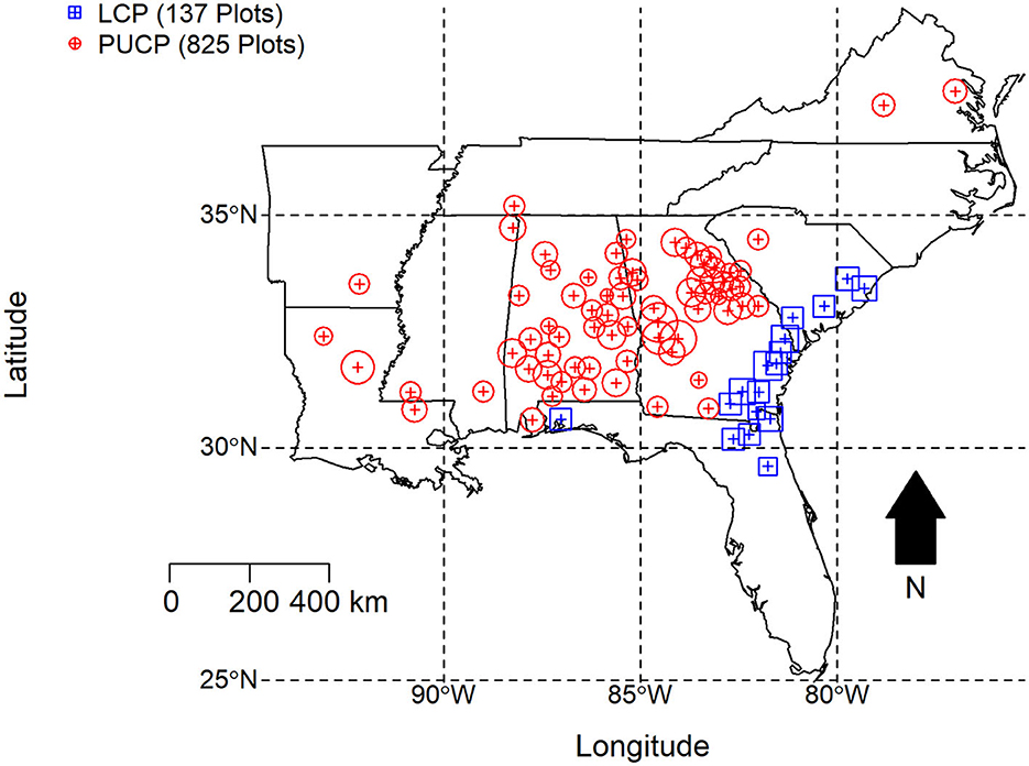
Figure 1. Growth and yield model installation location county centroids used to fit the PMRC 2014 growth and yield model. The area of the surrounding location correlates to the number of plots within that specific county, however only county centroids were used to fit the actual MaxEnt model.
Plots used to fit the PMRC 2014 growth and yield model include both traditional growth and yield installations and control plots from several different PMRC studies including the Coastal Plain Culture/Density Study (CPCD; Zhao et al., 2014) and the Consortium for Accelerated Pine Production Studies (CAPPS; Kinane, 2014). Plots were split into two different physiographic regions, PUCP and LCP. Overall, a total of 825 plots were used to fit the PUCP variant of the 2014 model. These plots are concentrated in Alabama and Georgia but extend as far west as Arkansas/Louisiana and as far north and east as Virginia. A total of 137 control plots were used the fit the LCP variant of the 2014 model. These plots are concentrated within the coastal plain of South Carolina, Georgia, and northeastern Florida; an additional six plots were included from northwestern Florida.
MaxEnt is a correlative modeling technique, hence it required duplicates within location to be removed to ensure that the prediction accuracy is not inflated. To achieve this, duplicate plots were removed from the data set allowing for only one centroid per county to be included. Duplicate removals reduced the total number of available centroid locations to 17 and 71 for the LCP and PUCP, respectively. Euclidean distances between each point in the two individual sets was calculated to assess the potential for spatial autocorrelation between the locations, an issue that results in biased predictions (Anderson, 2015). No occurrence localities were found to be within 20 km of each other so the collection installations were not spatially filtered for the LCP or PUCP sets of points. This threshold is within a range of values defined in similar studies that use MaxEnt to predict the potential distribution of a species or evaluated MaxEnt model tuning and selection criteria (Pearson et al., 2007; Anderson and Gonzalez, 2011; Shcheglovitova and Anderson, 2013; Boria et al., 2014; Radosavljevic and Anderson, 2014).
2.3. Biophysical data
2.3.1. Climatic information
Climatic data from the University of East Anglia's Climatic Research Unit (CRU TS4.01) was used for this analysis alongside PRISM (Parameter-elevation Relationships on Independent Slopes Model) climate data from Oregon State University (PRISM Climate Group, 2015).
2.3.2. CRU climate data
CRU TS4.01 is a gridded climate data set developed using the Climate Anomaly Method (CAM) to interpolate commonly used surface climate variables measured from meteorological stations across the globe into a half-degree, latitude/longitude grid (Harris et al., 2014). The CAM works by calculating a normal (average) across a period of time (typically 1961–1990, referred to as “climatology”) for each weather station that meets the strict inclusion criteria (Jones, 1994; Peterson et al., 1998; Harris et al., 2014). If a normal can be calculated for these 30 years, the station's series is included in the gridding process, and anomalies are calculated by differencing the 1961–1990 normal from the weather station's monthly data values. Two of the anomalies used in this analysis, precipitation and rain days, are calculated on a percent difference basis and do not use the above subtraction rule (Harris et al., 2014). The percent difference anomalies are calculated using a different reference period (1995–2002) and are then converted to the above 1961–1990 normal scale. Triangulated linear interpolation is then used to grid each anomaly at the half-degree resolution. Finally, each anomaly is converted back to an absolute value using one of two formulas depending on if they use the typical subtraction rule (Equation 1) or the percent difference rule (Equation 2):
where x is the absolute value, is the normal (as described above), and xa is the calculated anomaly.
Data for the CRU monthly climate data are primarily supplied by the World Meteorological Organization (WMO) and the National Climatic Data Center (NCDC) within the U.S. National Oceanographic and Atmospheric Administration (Harris et al., 2014). More specifically, data is collected from various data sets provided by the above organizations including: the CLIMAT monthly set (WMO), which pulls data from between 2200 and 2800 weather stations worldwide; the Monthly Climatic Data for the World (MCDW—produced by the NCDC), which collects data from an additional 1,500–2,600 weather stations; and data from the World Weather Records (WWR) in the form of decadal data publications exchanged between National Meteorological Services and the NCDC archive center. The first two sets, CLIMAT and MCDW are updated in near-real time, as mentioned WWR is available in decadal series, which (Harris et al., 2014) notes should theoretically match the monthly sets, but in practice, is cleaner than the monthly sets with fewer missing values and outliers.
CRU variables used in this analysis included minimum temperature (TMN), maximum temperature (TMX), precipitation total (PRE), vapor pressure (VAP), cloud cover (CLD), rain day counts (WET), potential evapotranspiration (PET), and the number of frost day (FRS). Here we offer a brief explanation for how each variable is calculated. However, in-depth explanations for each variable are found in Harris et al. (2014). TMN and TMX were calculated from absolute values of mean temperature and diurnal temperature range. PRE was calculated using the percentage anomalies multiplied by climatology and divided by 100, to which the climatology is added (2). VAP is derived using a calculated, “synthetic” VAP and station observed values for VAP. The synthetic VAP was calculated as a function of TMN. CLD is the cloud percentage cover; it was derived from diurnal temperature range anomalies coupled with CLD anomalies from the CLD station database to create 1995–2002 normal. This value was then adjusted to the 1961–1990 scale, and gridded absolute values were produced using the percent difference method described above. WET is calculated in a similar fashion to VAP, where a synthetic WET value is calculated as a function of precipitation and used in tandem with station-observed WET values to create the gridded data set. WET represents counts of wet days with ≥0.1mm of precipitation. FRS is estimated as a function of mean temperature and diurnal temperature rangeS and then constrained to ensure realistic measures alongside TMN. PET was calculated as a function of the mean temperature, TMN, TMX, VAP, CLD, and fixed wind speed using a variant of the Penman-Monteith equation.
Each monthly variable from the CRU data set was averaged from 1981 to 2010 to create a 30-year normal value that coincides with the 30-year normals from the PRISM data set. Conveniently, measurement dates for most of the data used to fit the PMRC 2014 Model fall within these 30 years.
2.3.3. PRISM climate data
PRISM (Parameter-elevation Relationships on Independent Slopes Model) is described as a knowledge-based system to interpolate climate data (Daly et al., 2008). It uses a regression-based approach along with point data from a large number of weather stations, a digital elevation model (DEM), other sets of data, and a “spatial climate knowledge base” to generate different climatic variables across the coterminous United States. Daly et al. (2008) offers an extensive summary of the methodology used to develop the 1971–2000 normal values for temperature and precipitation, while Daly et al. (2015) expands upon this approach and further describes the development of the 1981–2000 normals for vapor pressure deficit (both minimum and maximum) used in this analysis. PRISM uses a large number of weather station networks to estimate its vapor pressure elements. Because its normals are used for interpolating other climatic variables, they are subjected to intense peer review (PRISM Climate Group, 2015).
Only one climatic variable was taken from the PRISM data set, 30-year normal (1981–2010) average vapor pressure deficit (AVPD). AVPD was calculated by averaging the minimum vapor pressure deficit and maximum vapor pressure deficit normals.
2.3.4. Soils data
Three, easily accessible soil-derived predictors were used in this analysis, bulk density of the fine earth fraction (BD, kg m−3), percent clay (CLAY, percent weight), and percent organic carbon (SOC, percent weight). Bulk density was selected because of its relationship with root growth where it can become limiting once it crosses a certain threshold (Kelting et al., 1999; Will et al., 2002). Percent clay was selected because of its relationship with water (Rawls et al., 2003) and nutrient availability (Sampson et al., 2008). Soil organic carbon was selected based on its relationship with soil organic matter which has notable impacts on physical soil properties as well as chemical and biological composition as well (Johnsen et al., 2013).
Bulk density, percent clay, and soil organic carbon were selected from the data set created by Ramcharan et al. (2018) using a point data/machine learning approach to predict soil properties across the United States at seven different depths (0, 5, 15, 30, 60, 100, and 200 cm). Training data for this project was collected from three sources, the National Cooperative Soil Survey (NCSS) Characterization Database, the National Soil Information System (NASIS), and the Rapid Carbon Assessment (RaCA) Project. Data from these sources were used with various environmental covariates to develop 100 × 100 m predictive soil maps using two machine learning methods for classification, random forests, and gradient boosting. For the purpose of this analysis, the first four depths (0, 5, 15, and 30 cm) were combined to create an average bulk density to 30 cm depth (BD30), average percent clay to 30 cm depth (CLAY30), and an average percent organic carbon to 30 cm depth (SOC30). The 30 cm depth threshold was selected based on studies about loblolly pine rooting depth (Mou et al., 1995; Parker and Van Lear, 1996). For the reader's convenience, a table of commonly used abbreviations is listed below (Table 1).
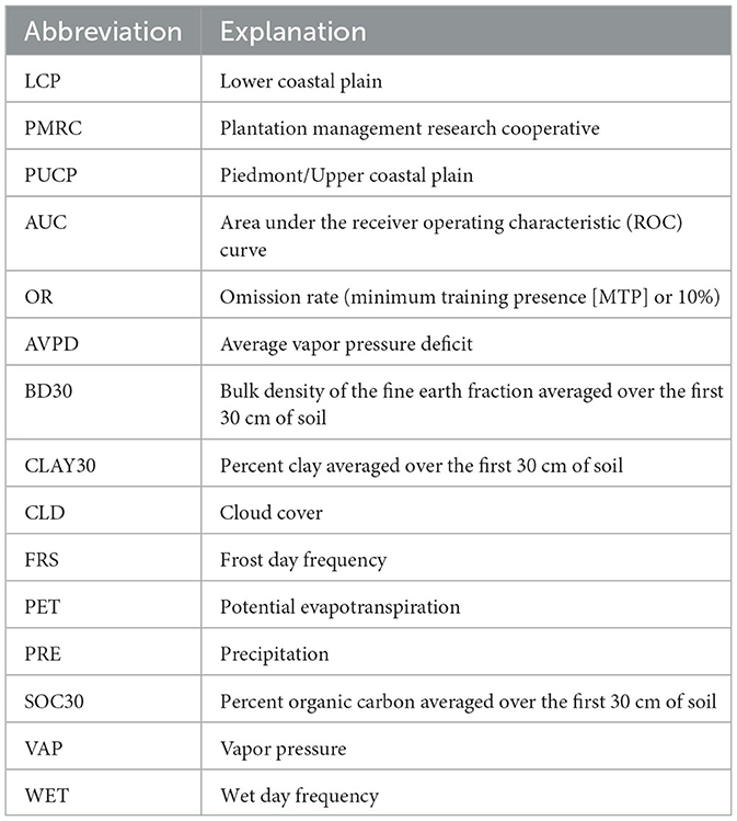
Table 1. Table of common abbreviations used throughout the paper.
2.3.5. Combining the climatic and soils data layers
Each set of predictors was first projected using the World Global Mercator—Spherical Mercator. This projection system was used to ensure that each cell was the same size across the entire study region as the half-degree resolution of the gridded climate data changes sizes with differing degrees of latitude. After reprojecting both data sets, the CRU climatic data (half-degree resolution), PRISM data (0.8 km resolution), and the soils data (initially at the 0.1 km resolution) were re-sampled to a 1 × 1 km resolution using bilinear interpolation. This was done because MaxEnt requires all predictors to have the same resolution. Bilinear interpolation was used for both data sets and produced reasonable smoothed surfaces, especially for the gridded climate data (Wang et al., 2006).
Each individual variable was then cropped and masked to the appropriate study areas previously described. The LCP variant of the model only included biophysical factors from Alabama, Florida, Georgia, and South Carolina. The PUCP variant included biophysical factors from the entire region shown in Figure 1. This is important because it also determines the landscape over which the evaluation background points are drawn.
Pearson's Correlation Coefficient (r) was used to examine the correlation between predictor variables. Though MaxEnt is equipped to handle highly correlated predictors (Elith et al., 2011; Merow et al., 2013), variables with correlation coefficients ≥ 0.90 were excluded from the model. Correlation coefficients for the original set of predictors are presented in Table 2. After evaluating correlation coefficients, the minimum temperature and maximum temperature were dropped from the analysis. These two variables were dropped because the number of frost days closely resembles the spatial patterns of both the minimum and maximum temperatures and because potential evapotranspiration includes average temperature in its calculation. Summary statistics for each potential predictor are presented in Table 3. All work in this section was completed using the raster package version 2.6–7 (Hijmans, 2017) in Microsoft R Open statistical software version 3.5.0 (Microsoft R Core Team, 2017).
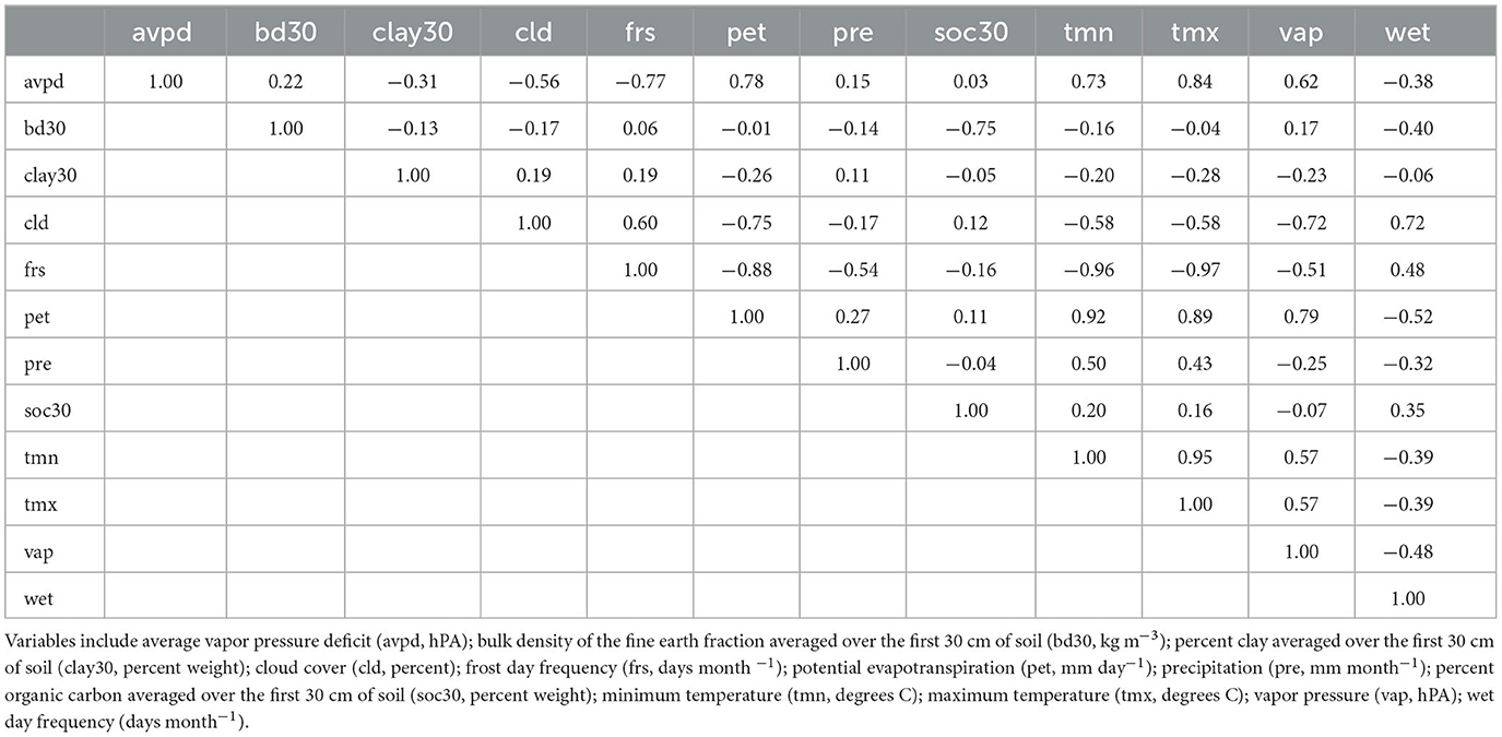
Table 2. Pearson Correlation Coefficients (r) for 12 environmental and soils variables.
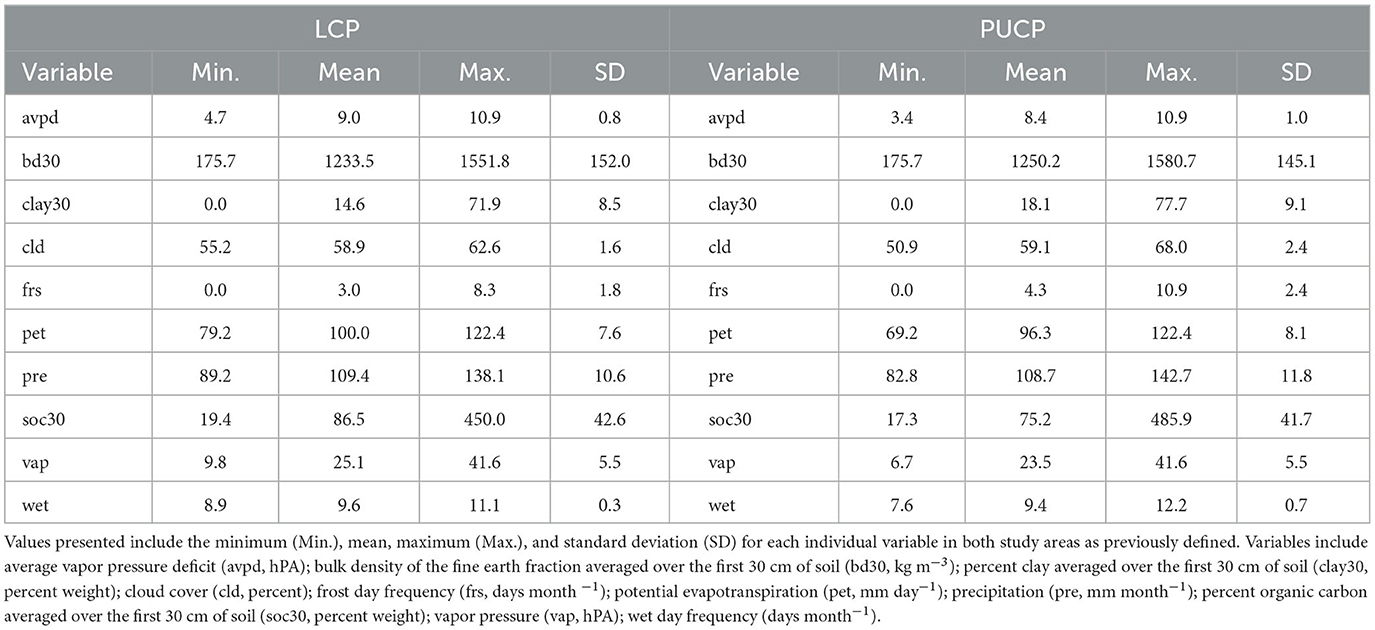
Table 3. Thirty year normal (1981–2010) climatic and soil variables used for the MaxEnt model for the Lower Coastal Plain (LCP) and Piedmont/Upper Coastal Plain (PUCP).
2.4. Maximum entropy models
Each maximum entropy model was trained using the MaxEnt algorithm version 3.4.1 (Phillips et al., 2018) in the dismo package version 1.1–4 (Hijmans et al., 2017) in Microsoft R Open statistical software version 3.5.0 (Microsoft R Core Team, 2017). The default model settings were used for the regularization multiplier (β = 1), convergence threshold, 10−5, maximum number of iterations, 500, and random background points used in the evaluation, 10,000. Feature types were included in the model based on the software's default rules relating to the number of provided presence points and included linear (L), quadratic (Q), and hinge (H) classes—product and threshold feature types were not included in this analysis. It is important to note that background points for the LCP simulations were drawn from only Alabama, Florida, Georgia, and South Carolina; background points from the PUCP simulations were drawn from the entire region depicted in Figure 1.
A detailed explanation of the software and all equations referenced in this section can be found in Dudík et al. (2004), Phillips et al. (2006), and Phillips et al. (2017). The Maxent software (Phillips et al., 2018) uses the principle described in the previous section along with a deterministic, sequential-update algorithm to estimate a probability distribution by determining the distribution of maximum entropy with respect to a set of constraining features (Dudík et al., 2004; Phillips et al., 2006). Applied to presence-only data, a user-specified study area is supplied to the software in the form of a pixelated or rasterized landscape along with recorded presence points and covariates such as environmental, soils, and physiographic data; the software then generates the maximum entropy distribution and overlays it across the pixels of the study area (Phillips et al., 2006). The entropy of the approximated distribution is written as:
where π represents the unknown, target distribution and represents its approximation over a finite set of pixels L. L represents the entire, user-defined landscape, and is composed of individual elements or points x.
The following represents an unconditional maximum entropy model and presents it through a machine learning framework. Though less common than conditional models in machine learning, the unconditional method must be used here due to a lack of absence data (Phillips et al., 2006). It should be noted that there are several papers that attempt to describe Maxent in a statistical framework that is much more similar to that seen in the statistical and ecological modeling literature (Elith et al., 2011; Merow et al., 2013) though these explanations are not presented here.
The Maxent software estimates the target probability distribution by imposing a set of constraints on the unknown probability distribution, π, through the use of features (transformed environmental variables, soils variables, etc.), fj, on L. Here, fj assigns a real value, fj(x) to all points x in L; the expectation of this feature under π is symbolized using π[fj]. Such expectations can be approximated by sampling from L, drawing xn number of points, independently. The probability distribution of maximum entropy is then defined as the approximated distribution, , with the constraint all features, fj, have the same mean under written as:
where the empirical mean of fj is expressed as and represents the uniform distribution on the sample points. This expectation is somewhat unrealistic and results in over-fit models as empirical feature means typically do not equal true feature means. The solution to this issue is addressed below.
A dual characterization of may also be defined using principles from mathematical optimization theory and convex duality (Della Pietra et al., 1997; Phillips et al., 2006; Elith et al., 2011). Considering probability distributions of the following form:
where λ is a vector of n feature weights, f is a vector of all real features, and Zλ ensures that qλ equals 1. This type of distribution is formally classified as a Gibbs distribution. Convex duality proves that the maximum entropy distribution, is equivalent to the qλ distribution that maximizes the likelihood of the m sample points, or minimizes the negative log likelihood of the sample points, described as the log loss function and written as:
or,
Relaxing the constraint in Equation (4) using a regularization multiplier allows the means under to vary slightly from the empirical mean (Dudík et al., 2004; Phillips et al., 2006). Doing so changes Equation (4) to:
where βj are some constants. Relaxing the constraint in Equation (4) also changes the log loss function from Equation (2.4) to a regularized log loss function of the form:
the second term here is a penalty and forces Maxent to focus on the most important features thus penalizing features with minimal contribution to the model. The goal of regularization here is to reduce model complexity to ensure that the model is not overly specific (Elith et al., 2011). Maxent uses a form of regularization known as l1-regularization that results in the reduction of overall terms in a model (Phillips et al., 2006; Elith et al., 2011), thus lowering its overall complexity and producing sparse models (James et al., 2013). Using the above loss function, Maxent starts from the uniform probability distribution and iteratively adjusts the weights to minimize the log loss function in order to compute the maximum entropy probability distribution.
The above formulation is equivalent to maximizing the likelihood of a parametric exponential distribution (Phillips et al., 2017). A recent evaluation of this formulation found that the same exact model can be derived from an inhomogeneous Poisson process (IPP) (Aarts et al., 2012; Fithian and Hastie, 2013; Renner and Warton, 2013; Phillips et al., 2017). Phillips et al. (2017) discusses the implications of this finding for modeling in great detail. For the purpose of this thesis, the most important implication is that the “raw” model output can now be interpreted as a model of relative abundance and can be transformed using a complimentary log-log (cloglog) transformation. This transformation is deemed appropriate because the predicted mean abundance in any given cell across the user defined landscape is modeled as a Poisson variable:
according to the Poisson distribution and as stated in Phillips et al. (2017), the probability of presence is therefore:
The above is a Bernoulli generalized model with a cloglog link function (Phillips et al., 2017). The largest caveat here is that the presence points are independent. This assumption should hold true for this analysis, although it is frequently violated in other studies relating to wildlife species based on sampling designs, etc., (Fithian et al., 2015; Renner et al., 2015). The cloglog transformation of the Maxent estimates is then:
where H represents the entropy, H = −Eλ[ln(pλ)], and pλ is the probability distribution. As previously mentioned this further extension of Maxent and its description as an IPP are discussed at great length in Phillips et al. (2017).
The models for each physiographic region were trained using a different occurrence partitioning method. The LCP model was fit using a jackknife technique (k−1 jackknife); this partitioning method is suitable for small data sets (Pearson et al., 2007; Kumar and Stohlgren, 2009; Shcheglovitova and Anderson, 2013) and was selected because of the small number of occurrence localities for this region. For the LCP, 17 different models were fit using 16 occurrence localities; the 17th locality was withheld and used as a test point to assess the model's performance. Thus, 17 different predictions were computed and then combined. The PUCP model was fit using the more traditional k-fold cross-validation, in this case five-fold cross-validation. Once again, model predictions were combined for all 5 models. Neither method considers the potential spatial autocorrelation between testing and training localities because none of the data collection locations were within 20 km of each other.
The area under the receiver operator curve (AUC) metric was used to assess the ability of both models as classifiers and is a rank-based, non-parametric measure of how well a model can distinguish presence points from random background points (Fielding and Bell, 1997; Phillips et al., 2006, 2017). This threshold-independent measure has an upper bound of 1 (Fielding and Bell, 1997) and considers both the sensitivity (probability of correct classification, P) and the specificity (probability of incorrect classification, 1-P) of a model; the AUC value's interpretation is, therefore, the probability that a model can correctly classify a random occurrence or a random background point (Phillips et al., 2006). An AUC value of 0.5 is no better than a random guess. A model producing a value of 0.75 is considered an adequate model (Graham and Hijmans, 2006; Pollock, 2015), though this threshold is somewhat arbitrary and is subject to change given a user's specific objectives. Two types of AUC values were evaluated, both AUCtrain, calculated using the training points, and AUCtest, calculated using the occurrence localities withheld from the training set for testing. Both AUC metrics were averaged across the k iterations; each was evaluated because AUCtrain is typically inflated for models with many parameters (Warren and Seifert, 2011). Because each model was fit to a different geographic extent, the LCP and PUCP model's AUC values are not comparable (Peterson et al., 2011), and the author acknowledges that AUC does not asses the overall fit of a model (Lobo et al., 2008; Peterson et al., 2011; Muscarella et al., 2014).
In an attempt to quantify overfitting, three different metrics were evaluated. All three were calculated following the procedures described in Muscarella et al. (2014). The first is the threshold-independent, average difference AUC metric (AUCdiff), calculated as the average difference between AUCtrain and AUCtest across all k folds (Warren and Seifert, 2011; Boria et al., 2014; Muscarella et al., 2014; Radosavljevic and Anderson, 2014). This metric is based on the premise that overly complex models should fit training data well but not necessarily testing data. Therefore, models with high AUCdiff values are positively correlated with overfitting. The other two methods are threshold-dependent metrics; the minimum training presence omission rate (ORMTP) and the 10% training omission rate (OR10; Pearson et al., 2007; Boria et al., 2014; Muscarella et al., 2014; Radosavljevic and Anderson, 2014). Omission rates are the proportion of testing locations incorrectly predicted when converted to a 0, 1 binary scale (Boria et al., 2014). The minimum training threshold sets the threshold value at the lowest prediction value for a training locality; if a locality in the test data set yields a prediction above this threshold it is identified as “suitable,” and assigned a value of 1 (Radosavljevic and Anderson, 2014). The omission rate is the proportion of testing locations with values below this threshold. The 10% threshold is similar except that the threshold value is set at whatever omits the 10% of training sites with the lowest predicted values. Lower omission rates typically express high model performance. Omission rates greater than the theoretical expected values are possibly subject to overfitting (Shcheglovitova and Anderson, 2013; Muscarella et al., 2014; Radosavljevic and Anderson, 2014).
3. Results
The MaxEnt model for the LCP had an AUCtrain value of 0.9524, and the average AUCtest across all jackknife simulations was 0.9080 with a corrected variance estimate of 0.0989 (Table 4). This variance is corrected for the non-independence of testing data across the jackknife simulations using the method described in Shao and Wu (1989) and discussed in Shcheglovitova and Anderson (2013) and Muscarella et al. (2014). AUCdiff for this model was 0.0547 with a corrected variance estimate of 0.0860. The minimum training presence threshold omission rate for this model was 0.2353, while the 10% training presence threshold omission rate for this model was 0.3529. These two values are higher than the expected theoretical values, implying that the LCP model might suffer from overfitting.
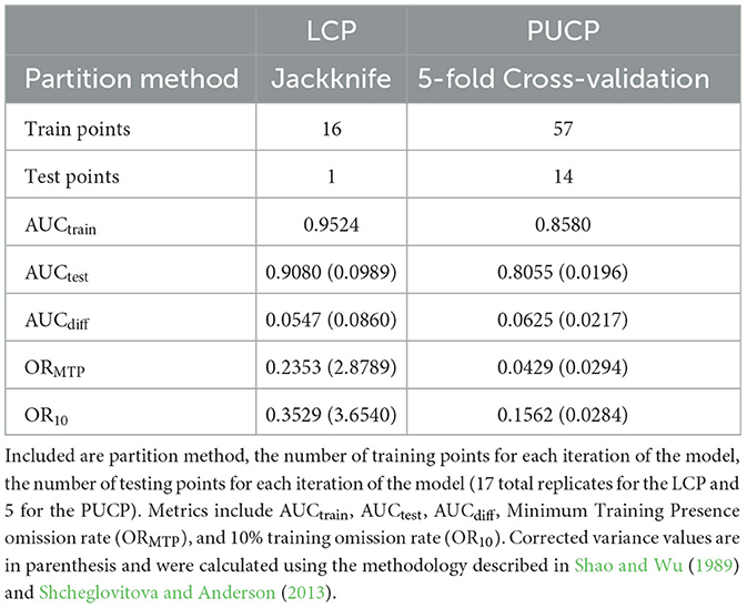
Table 4. Model information for each region (LCP and PUCP).
The estimated MaxEnt model for the LCP variant of the 2014 model utilized the soil organic carbon, percent clay, frost day frequency, cloud cover, precipitation, bulk density, average vapor pressure deficit, and wet day frequency predictors. Bulk density, precipitation, average vapor pressure deficit, and wet day frequency contributed <1% to the model. Potential evapotranspiration and vapor pressure were not used. The highest contributing variable for this model, as ranked by percent contribution, was soil organic carbon. Percent contribution and permutation importance for each predictor are presented in Table 5. The percent contribution is a heuristic estimate determined by the increase in gain to the model with respect to each individual variable (Baldwin, 2009). To determine the permutation importance the values for each variable are permuted randomly and the model is reevaluated using the new data, the drop in AUCtrain is calculated as a percent (Phillips et al., 2017). While they reveal pertinent information, especially the overall rank, these contributions can be heavily influenced by highly correlated variables and depend on the path the algorithm takes to the final solution. Because of this, the MaxEnt jackknife analysis for each variable included in the model was also evaluated. Results of the jackknife test of variable importance concur with those of the percent contribution values and are presented in Figure 2. This test revealed that the environmental variable that contains the most helpful information for the distribution is soil organic carbon because it increases the overall model gain when used by itself (blue bars in Figure 2). This same variable also results in the highest decrease in gain when omitted from the model, meaning it contains information not present in the other nine predictors (green bars in Figure 2). Thus, leaving this variable out notably changes the MaxEnt predictions (Pollock, 2015).
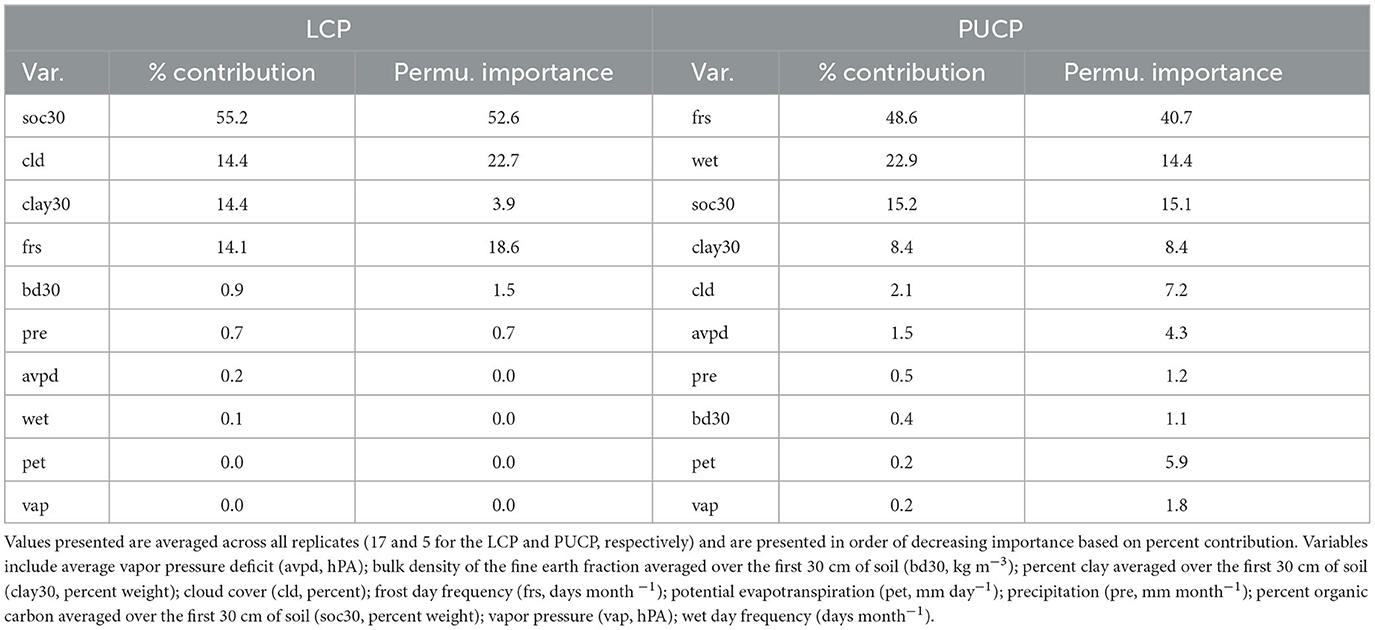
Table 5. Percent (%) contribution and permutation (Permu.) importance for each variable (Var.) in the MaxEnt model for each region.
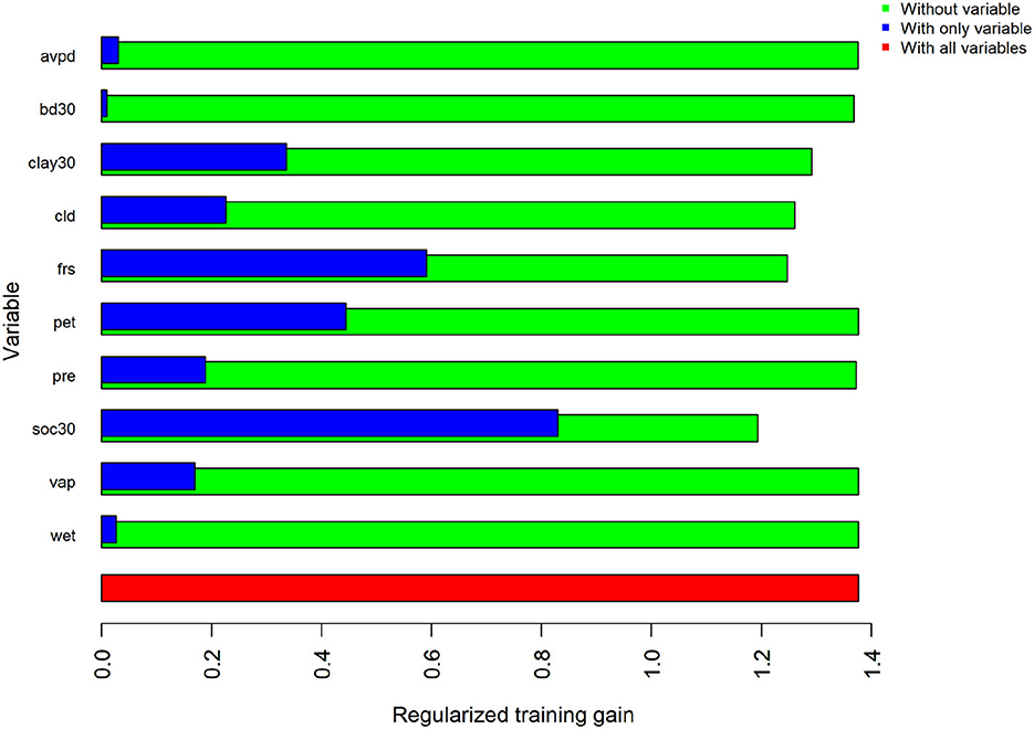
Figure 2. Results of the jackknife test of variable importance for regularized training gain in the LCP. Values shown are averages across all 17 replicates.
The MaxEnt model for the PUCP had an AUCtrain value of 0.8580, and the average AUCtest across all 5 replicates was 0.8055 with a corrected variance estimate of 0.0196 (Table 4). AUCdiff for this model was 0.0625 with a corrected variance estimate of 0.0217. The minimum training presence threshold omission rate for the PUCP model was 0.0429, while the 10% training presence threshold omission rate for this model was 0.1562.
The estimated MaxEnt model for the PUCP variant of the 2014 model utilized all ten available predictor variables; precipitation, bulk density, potential evapotranspiration, and vapor pressure all contributed <1%. Percent clay, cloud cover, and average vapor pressure deficit contributed <10%. The highest contributing variable for this model, as ranked by percent contribution, was the number of frost days. Percent contribution and permutation importance for each predictor are presented in Table 5. Once again, the jackknife test of variable importance was also evaluated for the PUCP model. Results from this test are illustrated in Figure 3. These results agree with the results of the percent contribution results. The variable that results in the highest gain when used by itself is the frost day frequency, conversely, it decreases the gain the most when excluded from the model.
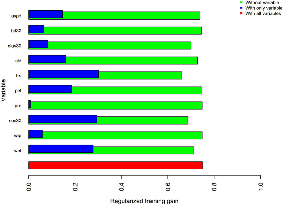
Figure 3. Results of the jackknife test of variable importance for regularized training gain in the PUCP. Values shown are averages across all five replicates.
Finally, complementary log-log (cloglog) prediction maps based on the selected models are illustrated for both regions in Figures 4, 5. As previously described, this transformation of the raw output values represents the “probability of occurrence” for that particular cell (Phillips et al., 2017), or for this particular use of MaxEnt it represents our level of confidence that the PMRC 2014 growth and yield model has the potential to characterize the growth that loblolly pine plantations correctly could experience across the given landscape. Warm-colored regions represent areas with similar environmental and soil characteristics to those at the occurrence localities.
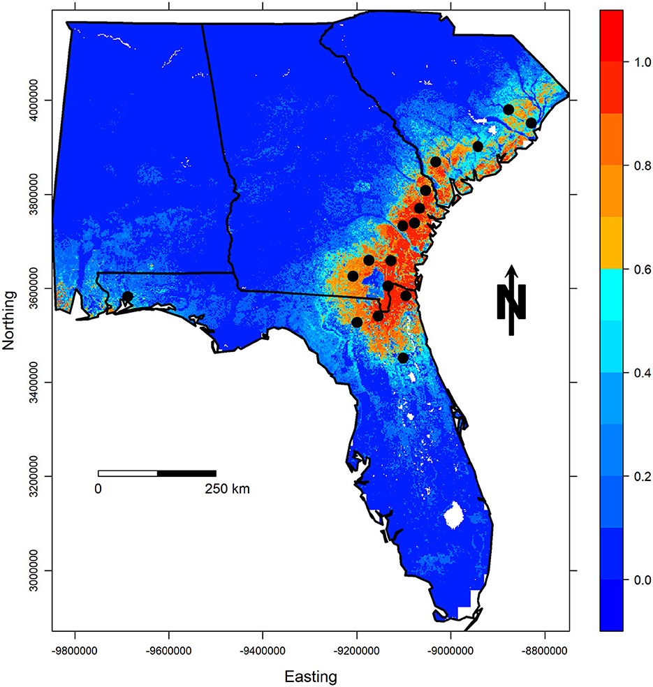
Figure 4. Cloglog probability of occurrence predictions for the best LCP model. Occurrence localities (county centroids) are shown in black.
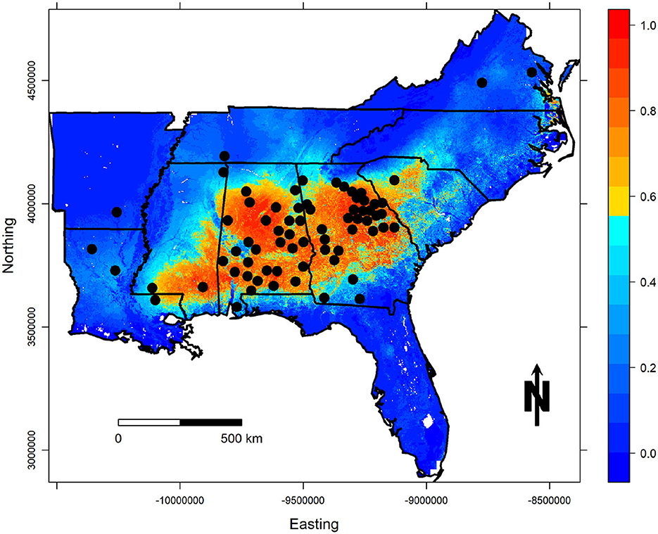
Figure 5. Cloglog probability of occurrence predictions for the best PUCP model. Occurrence localities (county centroids) are shown in black.
4. Discussion
Analyzing the output predictions for each individual model (Figures 4, 5) both seem to provide adequate predictions for the respective regions of the PMRC 2014 model. Unlike other approaches that typically label growth and yield models suitable for use in wide physiographic areas simply based on where data was collected to fit a growth and yield model, this technique provides explicit estimates of uncertainty for any location within the specified region. Users can then extract these estimates to determine how suitable the PMRC 2014 model might be for a given area allowing them to make better informed decisions based on their model predictions and projections.
The LCP model shows that many areas across the lower coastal plain of Georgia and parts of North Florida are very similar to the areas where data was collected to fit the model. Observers also note that the model is isolating the Okefenokee Swamp in South Georgia, which shows a very low probability of occurrence, a trend we would expect to see. Upon further investigation, this area has likely been omitted due to its notably different soil organic carbon levels in comparison with the rest of the region. Interestingly, the northern portion of the South Carolina LCP shows lower predicted suitability meaning that one or some of the environmental variables or an interaction between them is different from the other regions showing higher predicted values. Further evaluation of PMRC 2014 model predictions and projections should be conducted for this area to determine if any discrepancies exist in model predictions compared to growth data from this region. Another region that should be investigated is the southwestern portion of Florida and Alabama where despite being very small, there are some areas that show high suitability predictions. These locations have similar soil organic carbon values, cloud cover, frost day frequencies as the areas used to fit the model. Again, more work should be done to determine the validity of PMRC model predictions in these areas that are well outside the area described for this model's use.
The PUCP MaxEnt model shows high predicted values across the PUCP of Alabama, Georgia, and the upstate of South Carolina, despite the fact that only one installation in South Carolina was used to fit the PUCP variant of the PMRC 2014 model. The model also shows high predicted values for the southern Upper Coastal Plain of eastern Mississippi and some very small areas along the coast of southeastern Virginia and northeastern North Carolina; areas not prescribed for application in the model publication, but that have similar frost day frequencies and seasonal temperatures as the areas where data was collected to fit the PMRC PUCP model. The model shows low predicted values for the Ridge and Valley, Blue Ridge, and Appalachian Plateau physiographic region of Georgia; it also shows low predicted values for the Highland Rim and parts of the Cumberland Plateau in Alabama. The black-belt region and a majority of Louisiana and Arkansas were also identified as having low predicted values. These trends are expected and also make biological sense with respect to how loblolly pine plantations would be expected to grow differently in each of these regions (Hasenauer et al., 1994; Gallagher et al., 2019) based on their differing geologic formations, climates, and many other factors that influence growth.
AUC values for both models were above the previously described threshold of 0.75 at 0.9080 and 0.8055 for the LCP and PUCP models, respectively. Though the use of AUC to evaluate models has been argued both for and against, it does at least provide some measure of a model's overall ability as a classifier. The fact that both models returned average AUC values above the threshold supports the rationality behind each model (Pollock, 2015).
Results from both models show different conclusions with respect to overfitting. The LCP model, despite having a relatively high AUCtest value and a low AUCdiff value, appears to suffer from overfitting based on the ORMTP and OR10 metrics (Table 4). Both of these values are well above the theoretically expected values of 0.00 and 0.10 for the ORMTP and OR10 metrics, respectively. Were the regularization multiplier to be increased above the default value, these omission rates would likely drop as the model constraints would be loosened, however, no attempt was made to increase the regularization multiplier because of the context of use for the results from this maximum entropy model. In this case, an overfit model simply represents a conservative estimate of the areas we feel the PMRC 2014 model could be applied.
Unlike the LCP model, the PUCP model does not suggest overfitting with a low AUCdiff value and omission rate values close to the theoretical expectations (Table 4). The PUCP model also shows much lower levels of variability when compared with the LCP model for all four metrics evaluated in this study, this is likely in part due to the higher number of training localities available to fit the PUCP MaxEnt model.
The variables with the most significant impact for each model, as determined from both the percent contribution values (Table 5) and the jackknife contribution tests (Figures 2, 3), make biological sense when thinking about environmental and soils factors that influence the growth of loblolly pine in the southeastern United States. This is important because if a variable significantly contributes to a model, it likely contains differences across the region not found in the other predictor variables. Thus, ideally, these variables should have known importance for, or be related to a variable of importance for the species being evaluated.
In this case, both models found the soil organic carbon and frost day frequency predictors important in determining the maximum entropy distribution. SOC is directly related to soil organic matter (SOM), which helps to shape soil structure, chemistry, and biology (Johnsen et al., 2013) and is related to several important factors and processes in forest soils that can influence and regulate growth (Binkley and Fisher, 2013). These functions include water storage capacity (Rawls et al., 2003; Binkley and Fisher, 2013) along with nutrient pooling and cycling. It is also related to a site's drainage class. Frost day frequency follows a very similar geographic pattern to a minimum temperature which relates to growing season length and many physiologic processes that affect the growth of loblolly pine in the Southern United States (Nedlo et al., 2009).
Additionally, the LCP model found both the percent clay and cloud cover predictor variables to be important. Clay content can affect and influence many soil properties that affect loblolly pine, either directly or through complex interactions with many other soil factors. These processes and properties are related to soil chemistry (Binkley and Fisher, 2013), structure (Allen et al., 1990; Parker and Van Lear, 1996; Carlson et al., 2006), nutrient holding capacity (Fox et al., 2007), water storage capacity (Willett and Bilan, 1990), and many others. The cloud cover percentage variable is calculated using the diurnal temperature range alongside observed sun hours (Harris et al., 2014). While a bit less intuitive, this variable is related to solar radiation intensity and availability at Earth's surface (Matuszko, 2012) and thus the amount of solar radiation available for use by living organisms as photosynthetically active radiation (Cannell, 1989).
Similarly, the PUCP model also included percent clay, however, it also notably incorporated the wet day frequency predictor variable. The wet day frequency predictor variable shows the overall frequency of precipitation on a monthly basis (average days month−1 yr −1). When analyzed in conjunction with the precipitation layer used here, one can draw inferences about the intensity of overall rainfall events by comparing the wet day frequency and average precipitation for a given area. While this variable may have no seemingly direct link with loblolly pine, rainfall frequency, and intensity can affect a site's hydrological characteristics (Amatya et al., 2000; Amatya and Skaggs, 2001) such as excess water storage and soil saturation levels. The intensity of rainfall events may also influence nutrient cycling as well (Schreiber et al., 1990).
5. Conclusion
The work presented here uses a novel approach for defining the geographic bounds on growth and yield model usage based on different biophysical variables at the locations where data was collected to fit the model and across an area of interest. Using MaxEnt models for both the LCP and PUCP variants of the PMRC 2014 growth and yield model, this approach is able to better define geographic bounds on where we feel confident in the potential of the PMRC 2014 model to correctly characterize the growth experienced by loblolly pine plantations. This of course depends on these plantations being similar to those used to fit the model with respect to factors such as genetic material and silvicultural regimes.
The regularization multipliers were not adjusted for either model, hence the estimated ranges presented here represent conservative estimates of where the models should be used, especially for the LCP variant because its evaluation metrics suggest some level of overfitting. If an area falls outside of the predicted ranges presented here, it does not necessarily mean the PMRC 2014 model would not produce accurate growth predictions and projections for these areas as well, it simply means the predictor variables included in this work differ from those where data was collected to fit the models. Of course, regardless of the confidence one has in their growth and yield models, users should continually evaluate model outputs to ensure the most appropriate growth and yield model is being used for any area.
Further work needs to be completed to improve the tuning of MaxEnt models for this specific use. Additionally, a large-scale evaluation of PMRC 2014 growth and yield model predictions in areas the MaxEnt models are predicting as suitable vs. areas with lower prediction values could further validate the results of these MaxEnt models. Users may also use current and future environmental variables to project the areas suitable for PMRC model usage in the future. Adding in this temporal component could prove very useful for future management decisions and model deployment.
Data availability statement
The data analyzed in this study is subject to the following licenses/restrictions: The exact locations of the growth and yield plots are proprietary; however, county level information has been provided. Additionally, the climatic and soils datasets are publicly available and how to access these datasets is described in the article. Requests to access these datasets should be directed to WP, spencer.peay@uga.edu.
Author contributions
WP: conceptualization, methodology, validation, analysis, visualization, writing—original draft, and writing—review and editing. BB: conceptualization, methodology, validation, analysis, supervision, project administration, writing—review and editing, and funding acquisition. CM: conceptualization, methodology, validation, analysis, and writing—review and editing. All authors contributed to the article and approved the submitted version.
Funding
This work was provided by the Plantation Management Research Cooperative at the University of Georgia.
Acknowledgments
The authors would like to thank the Plantation Management Research Cooperative and its associated members.
Conflict of interest
The authors declare that the research was conducted in the absence of any commercial or financial relationships that could be construed as a potential conflict of interest.
Publisher's note
All claims expressed in this article are solely those of the authors and do not necessarily represent those of their affiliated organizations, or those of the publisher, the editors and the reviewers. Any product that may be evaluated in this article, or claim that may be made by its manufacturer, is not guaranteed or endorsed by the publisher.
References
Aarts, G., Fieberg, J., and Matthiopoulos, J. (2012). Comparative interpretation of count, presence-absence and point methods for species distribution models. Methods Ecol. Evol. 3, 177–187. doi: 10.1111/j.2041-210X.2011.00141.x
Allen, H. L., Dougherty, P. M., and Campbell, R. G. (1990). Manipulation of water and nutrients - practice and opportunity in southern U.S. pine forests. For. Ecol. Manage. 30, 437–453. doi: 10.1016/0378-1127(90)90153-3
Amatya, D. M., Gregory, J. D., and Skaggs, R. W. (2000). Effects of controlled drainage on storm event hydrology in a loblolly pine plantation. J. Am. Water Resour. Assoc. 36, 175–190. doi: 10.1111/j.1752-1688.2000.tb04258.x
Amatya, D. M., and Skaggs, R. W. (2001). Hydrologic modeling of a drained pine plantation on poorly drained soils. For. Sci. 47, 103–114.
Anderson, R. P. (2015). Modeling niches and distributions: It's not just “Click, Click, Click”. Biogeografia 8, 11–16.
Anderson, R. P., and Gonzalez, I. (2011). Species-specific tuning increases robustness to sampling bias in models of species distributions: an implementation with Maxent. Ecol. Model. 222, 2796–2811. doi: 10.1016/j.ecolmodel.2011.04.011
Baldwin, R. A. (2009). Use of maximum entropy modeling in wildlife research. Entropy 11, 854–866. doi: 10.3390/e11040854
Borders, B. E., Harrison, W. M., Shiver, B. D., and Daniels, R. F. (2014). Growth and Yield Models for Second/Third Rotation Loblolly Pine Plantations in the Piedmont/Upper Coastal Plain and Lower Coastal Plain of the Southeastern. U.S. Technical report. Athens, GA: University of Georgia.
Borders, B. E., Harrison, W. M., Zhang, Y., Shiver, B. D., Clutter, M., Cieszewski, C., et al. (2004). Growth and Yield Models for Second Rotation Loblolly Pine Plantations in the Piedmont/Upper Coastal Plain and Lower Coastal Plain of the southeastern U.S. - 2004. PMRC Technical Report, 63.
Boria, R. A., Olson, L. E., Goodman, S. M., and Anderson, R. P. (2014). Spatial filtering to reduce sampling bias can improve the performance of ecological niche models. Ecol. Model. 275, 73–77. doi: 10.1016/j.ecolmodel.2013.12.012
Burkhart, H. E., Amateis, R. L., Westfall, J. A., and Daniels, R. F. (2008). PTAEDA4.0: Simulation of Individual Tree Growth, Stand Development and Economic Evaluation in Loblolly Pine Plantations. Technical report, Forest Modeling Research Cooperative, Virginia Polytechnic Institute and State University, Blacksburg, VA.
Burkhart, H. E., Avery, T. E., and Bullock, B. P. (2019). Forest Measurements, 6th Edn. Long Grove, IL: Waveland Press.
Burkhart, H. E., and Tomé, M. (2012). Modeling Forest Trees and Stands. New York, NY: Springer. doi: 10.1007/978-90-481-3170-9
Cannell, M. (1989). Physiological basis of wood production: a review. Scand. J. For. Res. 4, 459–490. doi: 10.1080/02827588909382582
Carlson, C. A., Fox, T. R., Colbert, S. R., Kelting, D. L., Allen, H. L., and Albaugh, T. J. (2006). Growth and survival of Pinus taeda in response to surface and subsurface tillage in the southeastern United States. For. Ecol. Manage. 234, 209–217. doi: 10.1016/j.foreco.2006.07.002
Coble, D. W., Milner, K. S., and Marshall, J. D. (2001). Above- and below-ground production of trees and other vegetation on contrasting aspects in western Montana: a case study. For. Ecol. Manage. 142, 231–241. doi: 10.1016/S0378-1127(00)00353-4
Daly, C., Halbleib, M., Smith, J. I., Gibson, W. P., Doggett, M. K., Taylor, G. H., et al. (2008). Physiographically sensitive mapping of climatological temperature and precipitation across the coterminous United States. Int. J. Climatol. 28, 2031–2064. doi: 10.1002/joc.1688
Daly, C., Smith, J. I., and Olson, K. V. (2015). Mapping atmospheric moisture climatologies across the conterminous United States. PLoS ONE 10:e141140. doi: 10.1371/journal.pone.0141140
Della Pietra, S., Della Pietra, V., and Lafferty, J. (1997). Inducing features of random fields. IEEE Trans. Pattern Anal. Mach. Intell. 19, 380–393. doi: 10.1109/34.588021
Dudík, M., Phillips, S. J., and Schapire, R. E. (2004). “Performance guarantees for regularized maximum entropy density estimation,” in 17th annual Conference on Computational Learning Theory, 15.
Elith, J., and Leathwick, J. R. (2009). Species distribution models: ecological explanation and prediction across space and time. Annu. Rev. Ecol. Evol. Syst. 40, 677–697. doi: 10.1146/annurev.ecolsys.110308.120159
Elith, J., Phillips, S. J., Hastie, T., Dudík, M., Chee, Y. E., and Yates, C. J. (2011). A statistical explanation of MaxEnt for ecologists. Divers. Distrib. 17, 43–57. doi: 10.1111/j.1472-4642.2010.00725.x
Evans, M. E., Merow, C., Record, S., McMahon, S. M., and Enquist, B. J. (2016). Towards process-based range modeling of many species. Trends Ecol. Evol. 31, 860–871. doi: 10.1016/j.tree.2016.08.005
Fielding, A. H., and Bell, J. F. (1997). A review of methods for the assessment of prediction errors in conservation presece/absence models. Environ. Conserv. 24, 38–49. doi: 10.1017/S0376892997000088
Fithian, W., Elith, J., Hastie, T., and Keith, D. A. (2015). Bias correction in species distribution models: pooling survey and collection data for multiple species. Methods Ecol. Evol. 6, 424–438. doi: 10.1111/2041-210X.12242
Fithian, W., and Hastie, T. (2013). Finite-sample equivalence in statistical models for presence-only data. Ann. Appl. Stat. 7, 1917–1939. doi: 10.1214/13-AOAS667
ForesTech International LLC (2009). SiMS 2009 Suite of Software Products - Growth Model Documentation. ForesTech International LLC.
Fox, T. R., Jokela, E. J., and Allen, H. L. (2007). The development of pine plantation silviculture in the southern United States. J. For. 105, 337–347.
Gallagher, D. A., Bullock, B. P., Montes, C. R., and Kane, M. B. (2019). Whole stand volume and green weight equations for loblolly pine in the western Gulf Region of the United States through age 15. For. Sci. 2019:fxy068. doi: 10.1093/forsci/fxy068
Graham, C. H., and Hijmans, R. J. (2006). A comparison of methods for mapping species ranges and species richness. Glob. Ecol. Biogeogr. 15, 578–587. doi: 10.1111/j.1466-8238.2006.00257.x
Harris, I., Jones, P. D., Osborn, T. J., and Lister, D. H. (2014). Updated high-resolution grids of monthly climatic observations - the CRU TS3.10 dataset. Int. J. Climatol. 34, 623–642. doi: 10.1002/joc.3711
Harrison, W. M., and Borders, B. E. (1996). Yield Prediction and Growth Projection for Site-Prepared Loblolly Pine Plantations in the Carolinas, Georgia, Alabama and Florida. PMRC Technical Report. Athens, GA: University of Georgia.
Hasenauer, H., Burkhart, H. E., and Sterba, H. (1994). Variation in potential volume yield of loblolly pine plantations. For. Sci. 40, 162–176.
Hijmans, R. J., Phillips, S. J., Leathwick, J. R., and Elith, J. (2017). dismo: Species Distribution Modeling. R Package Version 1.1-4.
James, G., Witten, D., Hastie, T., and Tibshirani, R. (2013). An Introduction to Statistical Learning With Applications in R. New York, NY: Springer Texts in Statistics. doi: 10.1007/978-1-4614-7138-7
Jaynes, E. T. (1957). Information theory and statistical mechanics. Phys. Rev. 106, 620–630. doi: 10.1103/PhysRev.106.620
Johnsen, K. H., Samuelson, L. J., Sanchez, F. G., and Eaton, R. J. (2013). Soil carbon and nitrogen content and stabilization in mid-rotation, intensively managed sweetgum and loblolly pine stands. For. Ecol. Manage. 302, 144–153. doi: 10.1016/j.foreco.2013.03.016
Jokela, E. J., Dougherty, P. M., and Martin, T. A. (2004). Production dynamics of intensively managed loblolly pine stands in the southern United States: a synthesis of seven long-term experiments. For. Ecol. Manage. 192, 117–130. doi: 10.1016/j.foreco.2004.01.007
Jones, P. D. (1994). Hemispheric surface air temperature variations: a reanalysis and an update to 1993. J. Clim. 7, 1794–1802. doi: 10.1175/1520-0442(1994)007<1794:HSATVA>2.0.CO;2
Kelting, D. L., Burger, J. A., Patterson, S. C., Aust, W. M., Miwa, M., and Trettin, C. C. (1999). Soil quality assessment in domesticated forests - A southern pine example. For. Ecol. Manage. 122, 167–185. doi: 10.1016/S0378-1127(99)00040-7
Kinane, S. M. (2014). Consortium for accelerated pine production studies (CAPPS) 25 years of intensive loblolly pine plantation management (Master's thesis). University of Georgia, Athens, GA, United States.
Kumar, S., and Stohlgren, T. J. (2009). Maxent modeling for predicting suitable habitat for threatened and endangered tree Canacomyrica monticola in New Caledonia. J. Ecol. Nat. Environ. 1, 94–98.
Lobo, J. M., Jiménez-valverde, A., and Real, R. (2008). AUC: a misleading measure of the performance of predictive distribution models. Glob. Ecol. Biogeogr. 17, 145–151. doi: 10.1111/j.1466-8238.2007.00358.x
Matuszko, D. (2012). Influence of the extent and genera of cloud cover on solar radiation intensity. Int. J. Climatol. 32, 2403–2414. doi: 10.1002/joc.2432
Merow, C., Smith, M. J., and Silander, J. A. (2013). A practical guide to MaxEnt for modeling species' distributions: what it does, and why inputs and settings matter. Ecography 36, 1058–1069. doi: 10.1111/j.1600-0587.2013.07872.x
Mou, P., Jones, R. H., Mitchell, R. J., and Zutter, B. (1995). Spatial distribution of roots in sweetgum and loblolly pine monocultures and relations with above-ground biomass and soil nutrients. Br. Ecol. Soc. 9, 689–699. doi: 10.2307/2390162
Munro, H. L., Montes, C. R., Gandhi, K. J., and Poisson, M. A. (2022). A comparison of presence-only analytical techniques and their application in forest pest modeling. Ecol. Inform. 68:101525. doi: 10.1016/j.ecoinf.2021.101525
Muscarella, R., Galante, P. J., Soley-Guardia, M., Boria, R. A., Kass, J. M., Uriarte, M., et al. (2014). ENMeval: an R package for conducting spatially independent evaluations and estimating optimal model complexity for Maxent ecological niche models. Methods Ecol. Evol. 5, 1198–1205. doi: 10.1111/2041-210X.12261
Nedlo, J. E., Martin, T. A., Vose, J. M., and Teskey, R. O. (2009). Growing season temperatures limit growth of loblolly pine (Pinus taeda L.) seedlings across a wide geographic transect. Trees 23, 751–759. doi: 10.1007/s00468-009-0317-0
Parker, M. M., and Van Lear, D. H. (1996). Soil heterogeneity and root distribution of mature loblolly pine stands in piedmont soils. Soil Sci. Soc. Am. J. 60, 1920–1925. doi: 10.2136/sssaj1996.03615995006000060043x
Pearson, R. G., Raxworthy, C. J., Nakamura, M., and Townsend Peterson, A. (2007). Predicting species distributions from small numbers of occurrence records: a test case using cryptic geckos in Madagascar. J. Biogeogr. 34, 102–117. doi: 10.1111/j.1365-2699.2006.01594.x
Peterson, A. T., Soberon, J., Pearson, R. G., Anderson, R. P., Martinez-Meyer, E., Nakamura, M., et al. (2011). Ecological Niches and Geographic Distributions, Vol. 49. Princeton, NJ: Princeton University Press. doi: 10.23943/princeton/9780691136868.003.0003
Peterson, T. C., Karl, T. R., Jamason, P. F., Knight, R., and Easterling, D. R. (1998). First difference method: maximizing station density for the calculation of long-term global temperature change. J. Geophys. Res. Atmos. 103, 25967–25974. doi: 10.1029/98JD01168
Phillips, S. J., Anderson, R. P., Dudík, M., Schapire, R. E., and Blair, M. E. (2017). Opening the black box: an open-source release of Maxent. Ecography 40, 887–893. doi: 10.1111/ecog.03049
Phillips, S. J., Anderson, R. P., and Schapire, R. E. (2006). Maximum entropy modeling of species geographic distributions. Ecol. Model. 190, 231–259. doi: 10.1016/j.ecolmodel.2005.03.026
Phillips, S. J., and Dudík, M.. (2008). Modeling of species distribution with Maxent: new extensions and a comprehensive evalutation. Ecograpy 31, 161–175. doi: 10.1111/j.0906-7590.2008.5203.x
Phillips, S. J., Dudík, M., and Schapire, R. E. (2018). Maxent Software for Modeling Species Niches and Distributions (Version 3.4.1).
Pollock, J. J. (2015). A Maxent-based model for identifying local-scale tree species richness patch boundaries in the Lake Tahoe Basin of California and Nevada (Master's thesis). University of Southern California, Los Angeles, CA, United States.
PRISM Climate Group (2015). Descriptions of PRISM Spatial Climate Datasets for the Conterminous United States. Technical report, PRISM Climate Group.
Qin, A., Liu, B., Guo, Q., Bussmann, R. W., Ma, F., Jian, Z., et al. (2017). Maxent modeling for predicting impacts of climate change on the potential distribution of Thuja sutchuenensis Franch. An extremely endangered conifer from southwestern China. Glob. Ecol. Conserv. 10, 139–146. doi: 10.1016/j.gecco.2017.02.004
Radosavljevic, A., and Anderson, R. P. (2014). Making better Maxent models of species distributions: complexity, overfitting and evaluation. J. Biogeogr. 41, 629–643. doi: 10.1111/jbi.12227
Ramcharan, A., Hengl, T., Nauman, T., Brungard, C., Waltman, S., Wills, S., et al. (2018). Soil property and class maps of the conterminous United States at 100-meter spatial resolution. Soil Sci. Soc. Am. J. 82, 186–201. doi: 10.2136/sssaj2017.04.0122
Rawls, W. J., Pachepsky, Y. A., Ritchie, J. C., Sobecki, T. M., and Bloodworth, H. (2003). Effect of soil organic carbon on soil water retention. Geoderma 116, 61–76. doi: 10.1016/S0016-7061(03)00094-6
Renner, I. W., Elith, J., Baddeley, A., Fithian, W., Hastie, T., Phillips, S. J., et al. (2015). Point process models for presence-only analysis. Methods Ecol. Evol. 6, 366–379. doi: 10.1111/2041-210X.12352
Renner, I. W., and Warton, D. I. (2013). Equivalence of MAXENT and Poisson Point Process models for species distribution modeling in ecology. Biometrics 69, 274–281. doi: 10.1111/j.1541-0420.2012.01824.x
Restrepo, H. I., Bullock, B. P., and Montes, C. R. (2019). Growth and yield drivers of loblolly pine in the southeastern U.S.: a meta-analysis. For. Ecol. Manage. 435, 205–218. doi: 10.1016/j.foreco.2018.12.007
Sampson, D. A., and Allen, H. L. (1999). Regional influences of soil available water-holding capacity and climate, and leaf area index on simulated loblolly pine productivity. For. Ecol. Manage. 124, 1–12. doi: 10.1016/S0378-1127(99)00054-7
Sampson, D. A., Wynne, R. H., and Seiler, J. R. (2008). Edaphic and climate effects on forest stand development, net primary production, and net ecosystem productivity simulated for Coastal Plain loblolly pine in Virginia. J. Geophys. Res. 113, 1–14. doi: 10.1029/2006JG000270
Schreiber, J. D., Duffy, P. D., and McDowell, L. L. (1990). Nutrient leaching of a loblolly pine forest floor by simulated I. rainfall intensity effects. For. Sci. 36, 765–776.
Shao, J., and Wu, C. F. J. (1989). A general theory for jackknife variance estimation. Ann. Stat. 17, 1176–1197. doi: 10.1214/aos/1176347263
Shcheglovitova, M., and Anderson, R. P. (2013). Estimating optimal complexity for ecological niche models: a jackknife approach for species with small sample sizes. Ecol. Model. 269, 9–17. doi: 10.1016/j.ecolmodel.2013.08.011
Wang, T., Hamann, A., Spittlehouse, D. L., and Aitken, S. N. (2006). Development of scale-free climate data for western Canada for use in resource management. Int. J. Climatol. 26, 383–397. doi: 10.1002/joc.1247
Warren, D. L., and Seifert, S. N. (2011). Ecological niche modeling in Maxent: the importance of model complexity and the performance of model selection criteria. Ecol. Appl. 21, 335–342. doi: 10.1890/10-1171.1
Weber, T. C. (2011). Maximum entropy modeling of mature hardwood forest distribution in four U.S. States. For. Ecol. Manage. 261, 779–788. doi: 10.1016/j.foreco.2010.12.009
Weiskittel, A. R., Hann, D. W., Kershaw, J. A., and Vanclay, J. K. (2011). Forest Growth and Yield Modeling, 1st Edn. Hoboken, NJ: Wiley. doi: 10.1002/9781119998518
Will, R. E., Wheeler, M. J., Markewitz, D., Jacobson, M. A., and Shirley, A. M. (2002). II. Early loblolly pine stand response to tillage on the Piedmont and Upper Coastal Plain of Georgia: tree allometry, foliar nitrogen concentration, soil bulk density, soil moisture, and soil nitrogen status. Southern J. Appl. For. 26, 190–196. doi: 10.1093/sjaf/26.4.190
Willett, R. L., and Bilan, M. V. (1990). “Soil properties relating to height growth of loblolly pine on four major soil series in East Texas,” in Sixth Biennial Southern Silvicultural Research Conference (Memphis, TN), 458–469.
Yang, X. Q., Kushwaha, S. P., Saran, S., Xu, J., and Roy, P. S. (2013). Maxent modeling for predicting the potential distribution of medicinal plant, Justicia adhatoda L. in Lesser Himalayan foothills. Ecol. Eng. 51, 83–87. doi: 10.1016/j.ecoleng.2012.12.004
Keywords: maximum entropy (MaxEnt), growth and yield, geographic boundaries, southeastern United States, loblolly pine
Citation: Peay WS, Bullock BP and Montes CR (2023) A maximum entropy approach to defining geographic bounds on growth and yield model usage. Front. For. Glob. Change 6:1215713. doi: 10.3389/ffgc.2023.1215713
Received: 02 May 2023; Accepted: 25 September 2023;
Published: 10 October 2023.
Edited by:
Felipe Bravo, Universidad de Valladolid, SpainReviewed by:
Patrick Green, Virginia Tech, United StatesHans Pretzsch, Technical University of Munich, Germany
Copyright © 2023 Peay, Bullock and Montes. This is an open-access article distributed under the terms of the Creative Commons Attribution License (CC BY). The use, distribution or reproduction in other forums is permitted, provided the original author(s) and the copyright owner(s) are credited and that the original publication in this journal is cited, in accordance with accepted academic practice. No use, distribution or reproduction is permitted which does not comply with these terms.
*Correspondence: W. Spencer Peay, spencer.peay@uga.edu