Local adaptation, phenotypic plasticity, and species coexistence

1. Introduction

Spatial variation in the direction and strength of natural selection may often lead to eco-evolutionary dynamics. Local selection for the optimum phenotype could be hindered not only by gene flow but also from competitive interactions with other species; interactions which, in turn, could also be affected by the dual processes of gene flow and divergent selection (Hendry, 2017). Furthermore, theoretical models have shown that phenotypic plasticity, the ability of organisms to express different phenotypes depending on environmental conditions (Bradshaw, 1965; Schlichting, 1986), readily evolves when selective conditions are variable, whether in time or space (Hendry, 2017; Pfennig, 2021). In particular, spatial environmental variation where selection favors different phenotypes in each environment facilitates the evolution of adaptive phenotypic plasticity given some movement between environments (Via and Lande, 1985; Gomulkiewicz and Kirkpatrick, 1992; Scheiner, 1998). Since phenotypic plasticity occurs within an ecological context—e.g., a normal or helmet morph in water fleas depending on the absence or presence of predators (Agrawal et al., 1999), or quorum sensing in bacteria according to surrounding bacterial cell density (Miller and Bassler, 2001)—much current interest focuses on how variation in phenotypic plasticity can affect the dynamics of interacting populations or species (Fischer et al., 2014; Turcotte and Levine, 2016; Pérez-Ramos et al., 2019; Muthukrishnan et al., 2020; Start, 2020; Gómez-Llano et al., 2021).

Classical theory predicts that interspecific competition may select for traits that stabilize niche differences, weakening competitive interactions and therefore promoting species coexistence (Macarthur and Levins, 1967; Slatkin, 1980; Doebeli, 1996). However, recent work shows that ecological niche differentiation is not a requirement for species coexistence, and ecologically equivalent species can coexist when behaviors associated with reproductive interactions and sexual selection affect species demography in a frequency-dependent way (Gómez-Llano et al., 2021). On the other hand, the effect of phenotypic plasticity on species coexistence has been mainly framed within the classic context, in the sense that plasticity for ecologically relevant traits can eventually stabilize niche differentiation (Turcotte and Levine, 2016). Our aim here is to tackle the following question: does phenotypic plasticity affect species coexistence to the point that a competitively inferior plastic species can coexist with a competitively superior non-plastic one in the absence of niche differences? Specifically, we consider the following thought experiment: take an ecological model and contrast the community dynamics with or without intraspecific expressed variation for plasticity. When and why does variation change the dynamics? (Bolnick et al., 2011).

Here, we develop a computational model to investigate the effect of phenotypic plasticity on species' coexistence. We assume a density-compensating process which controls the size of the population (i.e., density-dependent population growth), coupled with a density- and frequency-independent viability selection for a local optimum that can be attained by adaptive phenotypic plasticity. We ran individual-based stochastic simulations using a two-dimensional landscape composed of spatially uncorrelated or autocorrelated environmental patches. We assumed two species: a competitively superior non-plastic species 1, that will always displace a second, phenotypically plastic species 2, in a single patch as well as in a two-dimensional landscape, with migration between patches but without environmental heterogeneity, which is temporally constant (i.e., when each patch has the same environmental value at each time step that defines the optimum phenotype). We mainly focus on the scenario where the two species are placed in a single random patch of a spatially heterogeneous and empty landscape, and thereafter are allowed to expand their ranges without being subjected to a competition-colonization trade-off (a well-studied mechanism for species diversity maintenance; Hastings, 1980; Calcagno et al., 2006; Muthukrishnan et al., 2020). Individuals of both species migrate to adjacent patches with the same probability per generation and have the same competitive strategies (i.e., the same absolute intra- and interspecific competition coefficients all over the patches) across the spatially varying landscape, but those patches with the highest average fitness contribute the most individuals (hard selection; Christiansen, 1975). A brief digression: here we refer to fitness in the evolutionary context of population genetics, and not as the average competitive ability as used in the framework of “modern coexistence theory” (Barabás et al., 2018). Intuition suggests that expressing phenotypic plasticity will enhance local adaptation (Scheiner, 1998, 2013), which could give some fitness advantage to the ecologically inferior plastic species and facilitate coexistence. Quantitative numerical results as well as qualitative analytical arguments support this intuition. In particular, we show that both species coexist in most patches provided the variance of the optimum phenotypes across patches and the migration probability are sufficiently large. This conclusion holds true even when plasticity was to a certain extent costly.

2. Model

Here, we describe an eco-evolutionary scenario to investigate the possibility of coexistence between two species when the ecological competition matrix violates the mutual invasibility condition for any given patch.

2.1. Spatial setting

We constructed an individual-based model to simulate a metapopulation of two multi-locus, haploid species that occupy discrete patches located on a 2-dimensional grid of linear length L and toroidal shape (a doughnut) to avoid edge effects. Each patch on the grid is characterized by an environmental value $E_i,i=1,\dots ,L^2$, which are random variables distributed by the multivariate normal distribution:

where $E^T=(E_1,\dots ,E_{L^2})$ and ${\mu }^T=({\mu }_1,\dots ,{\mu }_{L^2})$ is a vector whose elements are the expected values of the environmental values, i.e., E(E_i) = μ_i. Here, Σ is the covariance matrix whose elements are ${\Sigma }_{ij}=\sqrt{{\sigma }_i^2{\sigma }_j^2}{\rho }_{ij}$ where ${\sigma }_i^2$ is the variance of the environmental value at patch i and ρ_ij is the correlation between the environmental values at patches i and j, which we choose to depend on the Euclidian distance d_ij between those patches. Explicitly, we set ${\rho }_{ij}={\rho }^{d_{ij}}$ where ρ∈[0, 1] is the correlation between the environmental values of patches for which d_ij = 1. Of course, d_ij = 1 is the smallest distance between any two patches in the grid. We note that the correlation decreases exponentially with the distance between patches, i.e., ρ_ij = exp(−d_ij/ξ) where ξ = 1/|ln ρ| is the correlation length of the environment.

A word is in order about the calculation of the Euclidean distance d between two points (i₁, i₂) and (j₁, j₂) in a rectangular grid with cyclic boundary conditions (toroid). Let us assume that the open grid is L₁×L₂, i.e., that there are L₁ patches in the horizontal direction and L₂ in the vertical direction (L₁ = L₂ = L for the grid considered in this paper), so that i₁, j₁ = 1, …, L₁ and i₂, j₂ = 1, …, L₂. The horizontal and vertical distances between these points are given by the equations d_h = min (|j₁−i₁|, L₁−|j₁−i₁|) and d_v = min (|j₂−i₂|, L₂−|j₂−i₂|), from where we can readily calculate the Euclidean distance, viz., $d=\sqrt{d_h^2+d_v^2}$ .

To avoid a profusion of parameters we assume that the patches are statistically identical, i.e., μ_i = μ and ${\sigma }_i^2={\sigma }_e^2$ for i = 1, …, L². With this assumption we can set μ = 0 without loss of generality, since a different choice of μ would amount to a uniform shift on the environmental values and so it would be inconsequential. Although we set ${\sigma }_e^2=2$ in most of our simulations, we have also analyzed the effect of ${\sigma }_e^2$ on species' coexistence. We note that for ρ = 0 the environmental values E_i are statistically independent normal random variables with mean zero and variance ${\sigma }_e^2$. Most of our analysis will focus on the uncorrelated environment, but we have also analyzed the possibility of coexistence in environmentally autocorrelated landscapes (i.e., ρ>0). As a brief technical note, we mention that in the case the matrix Σ is symmetric and positive definite we can readily produce samples of the random vector E by setting E = μ+Σ^½X where ${\text{X}}^T=(X_1,\dots ,X_{L^2})$ is a random vector whose components are statistically independent standard normal random variables (Wasserman, 2004). The main difficulty here is the calculation of the square root of the matrix Σ, which can be done using its spectral decomposition.

2.2. Viability selection

Following Scheiner et al. (2020), the phenotype Z_i of an individual located at patch i at the time of development was determined by 40 haploid loci as

where R_k are the allelic values at the m_r = 20 non-plastic or rigid loci (i.e., loci whose phenotypic expression does not ontogenetically react to the environmental value), P_k are the allelic values at the m_p = 20 plastic loci (their phenotypic expression depends on external environmental cues that influence development) and ϵ is a normally distributed environmental effect with mean 0 and variance σ_ϵ = 1/10. Here, b is the plasticity parameter that takes on the value b = 0 for the non-plastic species (species 1) and b = 1 for the plastic species (species 2). There is no lack of generality in this choice because the allelic values P_k (and R_k as well) are real-valued variables and so any other choice of the plasticity parameter can be reset to b = 1 by a proper rescaling of P_k.

The initial allelic values for all loci were also independently drawn from a normal distribution with mean 0 and variance 1/10. Hence, the sum of allelic effects for each set of loci is a normal random variable of mean 0 and variance 20/10 = 2, which matches our typical choice for the variance of the environmental values, viz., ${\sigma }_e^2=2$. For a given genotype, the phenotype Z_i at patch i is a linear function of the environment value E_i and so $\sum _{k=1}^{m_r}{R}_k$ is the intercept and $b\sum _{k=1}^{m_p}{P}_k$ is the slope (Scheiner, 2013; Scheiner et al., 2020). In the initial setup, the expected values of these quantities are zero.

Selection is only for viability, and the survival probability of an individual at patch i depends on its phenotype and the cost of plasticity. Here, we assume a Gaussian fitness model (Scheiner et al., 2020):

where E_i is the optimum phenotype that coincides with the patch's environmental value (i.e., stabilizing selection with a moving optimum), w² is inversely proportional to the strength of stabilizing selection and c≥0 determines the cost of plasticity. Here, we set w² = 1 without loss of generality. In fact, we can easily eliminate the parameter w² from the model by rescaling the adaptive non-plastic allele values $R_k^{\prime }=R_k/w$ and the patches environmental values $E_i^{\prime }=E_i/w$. The adaptive plastic allele values P_k do not change. Since $E_i~N(0,{\sigma }_e^2)$, we have $E_i^{\prime }~N(0,{\sigma }_e^2/w^2)$. Hence, the effect of w² is simply a rescaling of the variance of the patches environmental values ${\sigma }_e^2$. In other words, increasing the strength of selection (i.e., decreasing w²) is equivalent to increasing ${\sigma }_e^2$ and hence to increasing the roughness of the landscape. Equation (3) includes maintenance costs of plasticity (DeWitt et al., 1998) because there is a proportional reduction in survival when c>0 even if plasticity is not expressed as it is the case for species 1. However, in this paper we assume that individuals belonging to species 1 do not carry plastic alleles, so effectively b = 0 and c = 0 for them.

We note that there are no intra and interspecific interactions during the viability selection process, whose net effect is to decrease the population of both species. After passing the viability selection process, the surviving individuals compete among themselves to repopulate their patch, as described next.

2.3. Ecological competition

We assume that when the two species occupy the same patch they interact and there is interference or scramble competition. Given the species abundances N_1i and N_2i in patch i = 1, …, L² after viability selection, the total number of offspring $N_{1i}^{\prime }$ and $N_{2i}^{\prime }$ produced by the individuals of each species is determined by Ricker's equations (Ricker, 1954):

where e^r is the maximum growth rate in a low-density population, K_max is the carrying capacity of each species when alone (assuming a₁₁ = a₂₂ = 1), and a_ij is the per capita effect of species j on species i (Godfray et al., 1991). For simplicity, here we assume that both species have the same maximum growth rate and equilibrium population size when alone in a patch.

In the absence of migration, so the individuals are confined to their birth patches, we consider the scenario where the non-plastic species (i.e., species 1) outcompetes the plastic species (i.e., species 2). This scenario is achieved by setting r∈(0, 2), a₂₁>a₁₁ and a₁₂<a₂₂. Furthermore, since we do not want to distinguish between the two species when only one species is present in the metapopulation, we set a₁₁ = a₂₂ = 1. To investigate the possibility of species coexistence (or lack thereof) when the ecologically inferior species 2 displays plasticity we set a₂₁ = 3/2, a₁₂ = 1/2 and r = 0.6 in our simulations. Assuming a relatively large r is reasonable in the case of expanding species as, e.g., insects (Frazier et al., 2006) and plants (Appendix in Franco and Silvertown, 2004). We emphasize that our choice for the competition matrix a excludes the possibility of mutual invasion, which is a standard requisite for species coexistence (Pásztor et al., 2006). In fact, since a₂₁ = 3/2>1 = a₁₁ species 1 can invade a resident population of individuals of species 2 at equilibrium, but since a₁₂ = 1/2 < 1 = a₂₂ species 2 cannot invade a resident population of individuals of species 1 at equilibrium. It is instructive to note that det(a) = 1/4>0, so our competition matrix offers a counterexample to the fallacious statement that det(a)>0 implies negative frequency dependence (i.e. rare advantage) and hence ensures mutual invasibility (TBox 9.1 in Pásztor et al., 2006).

We note that Ricker equations (4a) and (4b) yield real values for the number of offspring of each species in patch i = 1, …, L² and, in fact, the conditions that guarantee the superiority of species 1 over species 2 presented above for the single-patch situation are valid only when species numbers or abundances N_1i and N_2i are real variables. It turns out that transforming those real variables into integer variables that are necessary for our individual-based simulations may produce spurious results, such as permanence of a few individuals of species 2 in patches dominated by individuals of species 1 or the stability of patches dominated by individuals of species 2 against the invasion of a few individuals of species 1. Here, we circumvent this difficulty by taking the ceiling function in Equation (4a) (i.e., the least integer greater than or equal to $N_{1i}^{\prime }$) and the floor function in Equation (4b) (i.e., the greatest integer less than or equal to $N_{2i}^{\prime }$), which biases the competition in favor of species 1. In fact, this procedure impairs considerably the ability of species 2 to colonize a vacant patch i even when there is no competition (i.e., N_1i = 0) because a single founder of species 2 cannot produce more than one offspring for our choice of growth rate (r = 0.6). For instance, if there is a single adult individual of species 2 in an otherwise empty patch i (i.e., N_2i = 1 and N_1i = 0), then Equation (4b) yields $N_{2i}^{\prime }<{\mathrm{\text{e}}}^r\approx 1.8$. Since floor(1.8) = 1, a single founder of species 2 cannot populate a vacant patch. This effect is mitigated when the migration rate is large since in this case there is a good chance that several individuals of species 2 migrate together to the same patch. However, this is actually a convenient scenario for our purposes since the more ecologically impaired species 2 is, the more remarkable the finding that plasticity can guarantee its permanence in the metapopulation.

In addition, we set K_max as a hard upper bound to the number of offspring $N_{1i}^{\prime }$ and $N_{2i}^{\prime }$ in patch i. In other words, whenever $N_{li}^{\prime }>K_{max}$ we set $N_{li}^{\prime }=K_{max}$ for l = 1, 2. This procedure is actually inconsequential because the populations at each patch approach the support capacity K_max from below because of our choice of the growth rate (viz., r = 0.6). For Ricker's growth equation, overshooting and the possibility of limit cycles happens for r>2 only (see, e.g., Franco and Fontanari, 2017). In the Supplementary material, we present several instances of the time evolution of the species abundances that support our claim that N_li<K_max for l = 1, 2.

2.4. Reproduction

The ecological competition procedure described above determines the number of offspring of each species $N_{1i}^{\prime }$ and $N_{2i}^{\prime }$ in patch i = 1, …, L². We re-emphasize that although Equations (4a) and (4b) produce real values for the species abundances, we take the integer values of those abundances using the floor and ceiling functions with the care to bias the competition in favor of species 1 (see Section 2.3). Now we need to specify the phenotypes of the $N_{1i}^{\prime }$ offspring of species 1 and of the $N_{2i}^{\prime }$ offspring of species 2 in patch i. We assume that the individuals that passed the viability selection sieve reproduce asexually (see Supplementary Section 7 for a brief discussion of the effect of recombination) and that the mother of each offspring is chosen randomly, with replacement, among the survivors. We recall that the numbers of surviving individuals of species 1 and species 2 in patch i are N_1i and N_2i, respectively, and that all survivors have the same probability of being chosen as mothers regardless of their fitness. Hence, selection works at the level of survival (viability selection) only and not at the level of the (genetic) differences of reproduction of survivors. In this way the reproductive output reflects the ecological dynamics and not the population composition at each generation.

The differences between mother and offspring are due solely to mutations in the m_r non-plastic loci and in the m_p plastic loci, which were implemented as follows. Each allele of the offspring can mutate with probability u_r or u_p depending on whether it is a non-plastic or a plastic allele. (Here, we assume u_r = u_p = 5/1, 000, which gives a genome-wide mutation rate U = 0.2.) Once a mutation occurs, say at the plastic locus k, we add a normal random variable ξ of mean zero and variance 1/100 to the existing allelic value which then becomes P_k+ξ. This is Kimura's continuum-of-alleles model (Kimura, 1965). As usual, generations were discrete and non-overlapping. During the development of an individual in a particular patch, we ignored any potential influence of parental phenotypes as, e.g., transgenerational plasticity (Uller, 2008).

In sum, the offspring generation of species l = 1, 2 in patch i is obtained by selecting with replacement $N_{li}^{\prime }$ individuals from the N_li survivors of the selection sieve. The selected survivors are referred to as mothers. The phenotype differences between offspring and mothers are the mutations in the non-plastic and plastic loci.

2.5. Migration

Each individual within each patch can migrate to one of the eight surrounding patches (Moore neighborhood) with probability p_mig, and its destination is equally likely to be any of the eight patches. We were careful in keeping track migrant and non-migrant individuals that remained in their natal patch (Hassell et al., 1995). The flow of migrants between patches takes place simultaneously and it may result in some patches becoming empty or exceeding the carrying capacity. After arriving at their destination patches, the migrants as well as the residents of those patches pass the viability selection sieve as described in Section 2.2. Again, some patches may become empty at this stage.

2.6. Metapopulation dynamics

As originally defined by Levins (1969), metapopulation dynamics consists of the extinction and colonization of local populations. Early models analogous to Levins' showed that two competitors could coexist globally even if coexistence was impossible in a single patch (Levin, 1974; Slatkin, 1974; Nee and May, 1992). However, here we do not impose a random extinction probability; only local adaptation and gene flow may interact to promote genetic variation and coexistence in the metapopulation. Actually, real metapopulations may contain local populations that never go extinct (Schoener and Spiller, 1987). A cautionary note: Kawecki and Ebert (2004, p. 1232) rightly pointed out that “local adaptation is about genetic differentiation”, but warned to minimize non-genetic effects such as plasticity (thus considering it a “nuisance parameter”) when studying local adaptation. However, at the metapopulation level studied here the total phenotypic variation for plastic species 2 is the result of the variation in the reaction norm intercepts (first term on the right side of Equation 2) and slopes (second term on the right side of Equation 2), both of which have a genetic basis (Scheiner, 1993; Sommer, 2020). Therefore, local adaptation is better understood as how close the mean phenotype matches the patch's environmental optimum value.

In this paper we consider only an expanding population scenario. More pointedly, the initial population was located on a randomly selected patch of the 2-dimensional grid at carrying capacity K_max for the two species, each at equal frequency (i.e., K_max/2 individuals from each species), and all other patches were empty. We recall that the carrying capacity of the metapopulation is $K_{max}{L}^2$ individuals, so there is plenty of room for expansion from this initial setup. For each species independently, there was an equilibration period of 2,000 generations at the seed patch before the colonization of the empty patches started. We initialize the allelic values R_k, k = 1, …, m_r and P_k, k = 1, …, m_p in Equation (2) for each individual as described before. In the equilibration period the two species evolve independently in the seed patch, i.e., there is no interspecific (as well as intraspecific) competition since after viability selection one guarantees that there will be exactly K_max/2 offspring of each species. Thus, Equations (4a) and (4b) are not used in the equilibration period. In sum, during equilibration viability selection decreases the population of each species by eliminating the less fit individuals and reproduction resets the population of the seed patch to its original size.

After the equilibration period, the colonization of empty patches starts. The order of events is migration, phenotype determination, viability selection, ecological competition and reproduction. The sequence of these five events comprises one generation. Note that this sequence of events guarantees that a given individual undergoes the processes of selection, competition and reproduction within the same patch and that only their offspring have the possibility to migrate to neighboring patches.

A word is in order about the ecology that our model describes. Consider a particular patch, say patch i, at a moment just after migration, so its population consists of the offspring that stayed in patch i and those that migrated to patch i. We recall that the model assumes that only the offspring migrate. To reach the reproductive age, these offspring must pass the selection sieve in patch i. Those who passed this sieve become adults: they are the survivors, which amount to N_1i individuals of species 1 and N_2i individuals of species 2. The survivors compete among themselves in patch i to secure the resources to support their potential offspring. This competition is described in a coarse-grained manner by Equations (4a) and (4b), which output the number of offspring that each species can give rise to and sustain in patch i, viz., $N_{1i}^{\prime }$ and $N_{2i}^{\prime }$. At this point, we could argue that the survivors produce an infinite number of offspring but only $N_{1i}^{\prime }+N_{2i}^{\prime }$ of them survive because of resources limitation. Alternatively, we could argue that the survivors produce exactly the number of offspring determined by Equations (4a) and (4b). This last interpretation is the one adopted in population dynamics (Godfray et al., 1991; Pásztor et al., 2006), from where we have borrowed those Ricker-like equations. In any case, assuming one or the other scenario would not affect the outcomes. Next, the mothers of the $N_{1i}^{\prime }+N_{2i}^{\prime }$ offspring are chosen randomly with replacement among the survivors of each species. Behind the coarse-grained approach is the assumption that adults of the same species are indistinguishable with respect to their competitive and reproductive abilities. Finally, each offspring decides if it will stay in patch i or move to one of the neighboring patches.

2.7. Computer simulations

Individual-based simulations were independently implemented in Fortran and in MATLAB (2020) algebra environment using tools supplied by the Statistics Toolbox. Simulation results were double-checked by different authors to avoid any potential error. The results presented here are based in the Fortran code because it has speed advantages over MATLAB. The variable parameters were: L (landscape dimensionality), ${\sigma }_e^2$ (variance of the environmental values E_i), ρ (environmental correlation), K_max (patch's carrying capacity), c (plasticity cost), and p_mig (migration probability). For each set of conditions, we run 1,000 independent simulations (a random landscape for each simulation). The metapopulation dynamics was run for at most 2,100 generations and we used the last 100 generations to average over the quantities of interest (e.g., the abundance of each species) in the equilibrium regime. If one of the two species fixed before that upper limit, we halted the dynamics. Otherwise, we considered that coexistence was achieved. However, in the study of the single-species metapopulation dynamics all runs reached the upper limit of 2,100 generations. In the Supplementary material, we present many instances of the time evolution of both species (e.g., Supplementary Figure 12), which show that the running time of 2, 000 generations is sufficient to guarantee that the metapopulation dynamics reaches the equilibrium regime.

Since the quantities used to characterize coexistence at equilibrium are averages over patches (typically L² = 400), last generations of the colonization stage (100) and runs (typically 500 runs result in coexistence), the number of samples used to estimate their mean values is very large, resulting in error bars smaller than the sizes of the symbols used in the figures. However, in order to assess the variability of the equilibrium variables described next, in Supplementary Section 8, we offer a variety of scatter plots for selected values of the model parameters.

2.8. Equilibrium variables

In this paper we aim at the characterization of the metapopulation in the equilibrium regime, defined as the regime between generations t = 2, 000 and t = 2, 100. In the Supplementary material, we present results for the time evolution of both species in a variety of scenarios, but here we consider the equilibrium regime only. We focus on the following four variables.

• The mean relative abundances of each species, which we denote by 〈〈n_l〉〉 for l = 1, 2. These are the natural variables to describe the metapopulation at equilibrium. For p_mig>0, 〈〈n_l〉〉 is measured by averaging the number of individuals of species l (just after viability selection) over all patches during the last 100 generations of the 2,100 generations runs. The result is then divided by the number of patches (L²) and by the patch's carrying capacity (K_max). The same procedure applies for p_mig = 0, except that we must omit the division by the number of patches since the population cannot leave the seed patch in this case. The final result is then averaged over the independent runs. We represent all those averages by a double brackets notation. In the Supplementary material, we introduce a single bracket notation to discuss results for single runs. We note that all patches are considered in the computation of the mean relative abundances, regardless of whether they are empty, contain a single species or contain both species.

• The fraction of runs Γ for which there is coexistence at generation 2, 100. This quantity essentially measures the fraction of runs for which species 2 is not extinct, since even for rugged environments and large migration probabilities, species 1 is rarely extinct. For a run to result in coexistence it is enough that both species are present in the metapopulation at t = 2, 100. Hence, Γ offers no information whatsoever on the nature of the coexistence, i.e., whether the two species coexist within a same patch or inhabit different patches. We stress that there is no averaging procedure involved in the evaluation of Γ.

• The mean fraction of patches 〈〈Π〉〉 that carry both species for the runs that led to coexistence. For each run, an average is calculated over the last 100 generations of the run and then the result is averaged over runs. Hence, the double brackets notation. Clearly, 〈〈Π〉〉 offers valuable information on the nature of coexistence. Values of 〈〈Π〉〉 close to 1 indicate that most patches harbor both species, whereas values of 〈〈Π〉〉 close to 0 indicate that coexistence may take place in only a few patches due perhaps to their extreme environmental values that prevent their colonization by species 1. We refer to the former type of coexistence as within-patch coexistence and to the latter type as among-patch coexistence. The variable 〈〈Π〉〉 allows us to distinguish between these two types. We advance that within-patch coexistence is predominant at intermediate values of the migration probability p_mig and of the environment roughness ${\sigma }_e^2$, whereas among-patch coexistence becomes more important at low and high levels of those parameters.

To facilitate the interpretation of these variables, in Supplementary Section 3, we offer snapshots of the grid where the abundances the two species in each patch is shown in a color scale.

3. Results

3.1. Single-species metapopulation dynamics

As the uncertain heterogeneous environment poses an adaptive challenge to both species through the viability selection sieve, it is instructive to study the metapopulation dynamics separately for each species before considering the competition between them. In addition, for the runs that do not result in coexistence, the equilibrium of the metapopulation is described by the single-species dynamics. As before, the initial single-species population was located on a randomly selected patch of the 2-dimensional grid at carrying capacity K_max and there was an equilibration period of 2,000 generations before the individuals were allowed to migrate to the neighboring patches.

3.1.1. Non-plastic species

Let us consider first the dynamics of the non-plastic species 1, which is obtained by setting b = 0 in Equation (2), c = 0 in Equation (3), and N_2i = 0 in Equations (4a) and (4b).

The effects of the migration probability and environmental correlation on the mean relative abundance of species 1 are summarized in Figure 1. There is a steady decrease of 〈〈n₁〉〉 with increasing p_mig, which is clearly a consequence of the difficulty of the non-plastic species to adapt to the heterogeneous patches. This happens in part because some lineage branches of a migrant individual (ancestor) have not enough time to adapt to their local environment since the individuals are forced to migrate to neighboring patches. However, some lineage branches are likely to stay and to adapt to their local environment. But a fraction of the population of these well-adapted lineages are continually transferred to patches where they are poorly adapted and the individuals have little chances of surviving and hence of sending offspring back to the patch of their ancestors. In that sense, migration produces an effective fitness independent culling of individuals of species 1. This problem is mitigated when the environment is highly correlated, i.e., the environmental values at neighboring patches are likely to be very similar, and disappears altogether for a homogeneous environment (ρ = 1). The finding that the non-plastic species reaches only a fraction of the maximal patch occupancy is key to explaining coexistence in our model: the dashed horizontal line in Figure 1 indicates the population density below which the non-plastic species cannot prevent the invasion of the plastic species, as will be shown in Section 3.2.2.

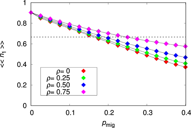
Figure 1. Mean relative abundance of the non-plastic species 〈〈n₁〉〉 for the single-species metapopulation dynamics as function of the migration probability p_mig for the environmental correlation ρ = 0, 0.25, 0.5, and 0.75, as indicated. The other parameters are L = 20, K_max = 100 and ${\sigma }_e^2=2$. The lines connecting the symbols are guides to the eye. The dashed horizontal line is 〈〈n₁〉〉= 1/a₂₁ = 2/3.

In the case the population is confined to the seed patch (i.e., for p_mig = 0) we find 〈〈n₁〉〉≈0.9. The adaptation is not perfect due to the noise ϵ in Equation (2) and to the non-zero genome-wide mutation probability U. (We note that since the genome of species 1 is determined by the m_r = 20 non-plastic alleles R_k only, and since each allele has probability u_r = 5/1, 000 of mutating we have U = 0.1.) Of course, this reduction in fitness caused by mutations is the well-known mutational load effect (Crow, 1958). It is instructive to quantify the effect of ϵ on the survival probability of an individual of species 1 carrying the optimal phenotype in the seed patch i. In this case, $Z_i^{opt}=E_i+ϵ$ and so $W_i^{opt}={\mathrm{\text{e}}}^{-{ϵ}^2/2}$. Recalling that ϵ~N(0, σ_ϵ), the expected survival probability of the optimal phenotype is

which yields $E(W_i^{opt})\approx 0.95$ for ${\sigma }_{ϵ}^2=1/10$.

The probability of metapopulation extinction was essentially zero for species 1, except for large values of the migration probability (i.e., p_mig>0.35). For instance, for p_mig = 0.4 we find that only 8 out of the 1, 000 runs resulted in extinction for ρ = 0, whereas no extinction was observed for ρ = 0.75. In Supplementary Section 1, we discuss the adaptation process of species 1 with emphasis on the time dependence of the sum of the non-plastic allelic values $\sum _k{R}_k$ and to the mean fitness of the population.

3.1.2. Plastic species

We turn now to the dynamics of the plastic species 2, which is obtained by setting b = 1 in Equation (2), and N_1i = 0 in Equations (4a) and (4b). The setup is the same as described in the study of the non-plastic species.

Figure 2 shows that the migration probability and the environmental correlation have no effect on the relative abundance of the plastic species 2 in the case plasticity is costless (c = 0). This unexciting finding is actually important because it validates our modeling of the plastic species. In fact, a plastic species should thrive equally well in all patches (hence the unresponsiveness to changes on p_mig), regardless of the environment (hence the unresponsiveness to ρ), as observed in Figure 2. In addition, these results already illustrate the fitness advantage of the plastic species 2 over the non-plastic species 1, specially for large migration probability. Here, we use the relative abundance of the species after viability selection as a proxy for the fitness of the species. Of course, adaptation of species 2 mainly happens via the contribution of the plastic components P_k to the mean optimum phenotype and this is achieved by setting the non-plastic components R_k as close to zero as possible. In Supplementary Section 2, we offer a study of the adaptation process of species 2 with emphasis on the time dependence of the sum of both non-plastic $\sum _k{R}_k$ and plastic $\sum _k{P}_k$ allelic values as well as of the mean fitness of the population. We note that for p_mig = 0, we find 〈〈n₂〉〉≈0.87, which indicates that species 2 is slightly less well-adapted to the environment of the seed patch than species 1. The probable reason for this is that the genome-wide mutation probability for species 2 is twice that of species 1.

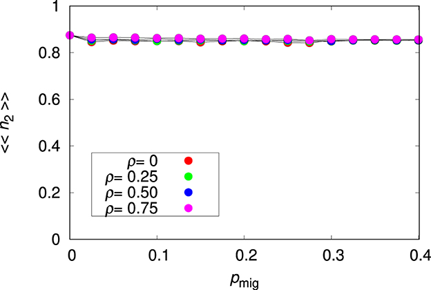
Figure 2. Mean relative abundance of the plastic species 〈〈n₂〉〉 for the single-species metapopulation dynamics as function of the migration probability p_mig for the environmental correlation ρ = 0, 0.25, 0.5, and 0.75, as indicated, and plasticity cost c = 0. The other parameters are L = 20, K_max = 100 and ${\sigma }_e^2=2$. The lines connecting the symbols are guides to the eye.

The invariance of 〈〈n₂〉〉 to changes in p_mig and ρ does not hold when there is a cost to plasticity (i.e., c>0), as shown in Figure 3. This is expected because introducing a cost to plasticity makes species 2 less plastic and hence more similar to species 1. In fact, in order to maximize survival for large c, the allelic values P_k must tend to zero, thus reducing the influence of the penalty term in Equation (3). Of course, setting the values of the plastic alleles to zero is equivalent to turning species 2 into a non-plastic species (see Supplementary Figure 6). For p_mig = 0 and c>0 the optimal phenotype is R_k = E_i, ∀k and P_k = 0, ∀k where i the seed patch. This result can be obtained by the direct maximization of W_i, given in Equation (3), with respect to R_k and P_k. For p_mig>0, there is a trade-off between R_k and P_k: for small c it is advantageous to explore plasticity (see Figures 1, 2), whereas for large c it is advantageous to turn off the plastic alleles. Although in the latter case species 2 becomes essentially a non-plastic species, we note that 〈〈n₂〉〉 is slightly below 〈〈n₁〉〉 because of the practical impossibility to keep P_k close to zero due to the persistent perturbations produced by the mutation process.

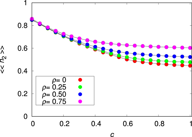
Figure 3. Mean relative abundance of the plastic species 〈〈n₂〉〉 for the single-species metapopulation dynamics as function of the plasticity cost c for the environmental correlation ρ = 0, 0.25, 0.5, and 0.75, as indicated, and migration probability p_mig = 0.3. The other parameters are L = 20, K_max = 100 and ${\sigma }_e^2=2$. The lines connecting the symbols are guides to the eye.

We advance that, somewhat surprisingly, the plasticity cost will be crucial to the interpretation of the results of the interspecies competition in our model. In fact, as already mentioned without evidence, if the relative abundance of species 1 in a given patch is less than some threshold value, the resident species cannot prevent the invasion of (and the consequent coexistence with) a competitively inferior species. However, we will show next that control of the fitness of species 2 using the parameter c (see Figure 3) indicates that successful invasion requires the invading species to be very well-adapted to the patchy environment.

In time, we say that a species is competitively inferior if it cannot invade a resident population of the other species in a single-patch scenario (i.e., for p_mig = 0). In that sense, competitive superiority or inferiority is completely determined by the competition matrix a introduced in Section 2.3. Also, by fitness of a species we mean the relative abundance of the species after viability selection, which is given by averaging the survival probability, Equation (3), over individuals, patches, and generations at equilibrium.

3.2. Two-species metapopulation dynamics

We consider now the general setup where the two species are first let to reach equilibrium independently of each other in the seed patch and then are allowed to compete and migrate to the neighboring patches. Of course, the focus here is on the runs that led to coexistence since the runs that do not lead to coexistence were already fully characterized in the previous subsection.

Figure 4 summarizes the effects of the environment on the probability that a run results in coexistence, which is measured by Γ (Figure 4A), and on the fraction of patches that harbor the two species, which is measured by 〈〈Π〉〉 (Figure 4B). To a good approximation the effect of the environment is represented by the single variable ${\sigma }_e^2(1-\rho )$, which means that ρ can be absorbed in ${\sigma }_e^2$ and we can study the uncorrelated landscape only without loss of generality. In other words, increasing the correlation between patches is equivalent to decreasing the variance of environmental values in an uncorrelated landscape. The important message from Figure 4 is that the plastic species 2 is extinct in a quasi-homogeneous or smooth environment (i.e., for ${\sigma }_e^2(1-\rho )\approx 0$). We note that in this region there are no data for 〈〈Π〉〉 because no run resulted in coexistence.

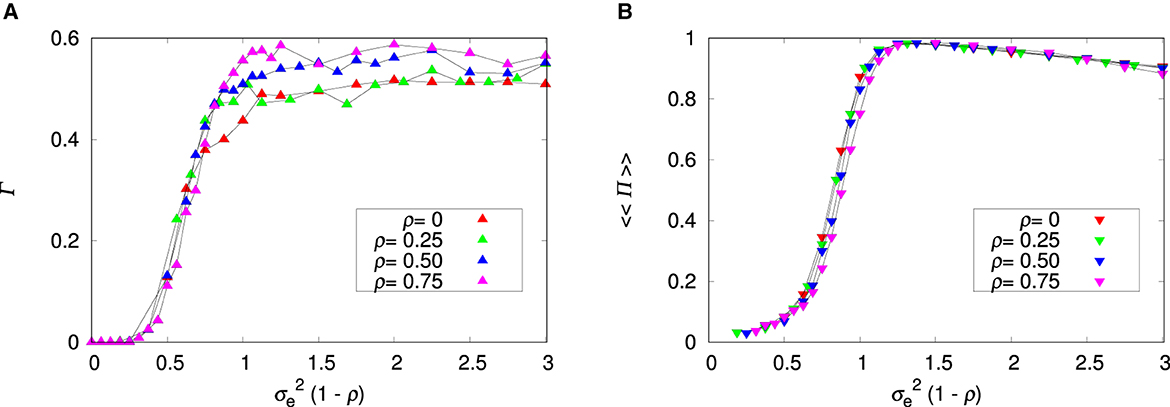
Figure 4. Influence of the variance of environmental values ${\sigma }_e^2$ and patch's environmental correlation ρ on species coexistence. (A) Fraction of runs that led to species coexistence. (B) Fraction of patches where there is species coexistence. The parameters are L = 20, K_max = 100, c = 0, and p_mig = 0.3. The lines connecting the symbols are guides to the eye.

Interestingly, increase of the environment roughness has only a limited effect on the probability of coexistence Γ, which quickly levels out and remains unaffected by further changes on ${\sigma }_e^2$ (Figure 4A). The probability that a patch exhibits coexistence 〈〈Π〉〉 displays a more interesting behavior (Figure 4B). For smooth environments, most patches are occupied by species 1 only, but as the environment roughness increases, those patches begin to harbor both species. The slow decrease of 〈〈Π〉〉 we observe for large ${\sigma }_e^2$ is due to the appearance of patches occupied by species 2 only (see Supplementary Figures 9–11).

Figure 5 shows the environmental effect on the relative abundances of both species. For smooth environments, species 2 is present in a few patches only (Figure 4B) and so its relative abundance 〈〈n₂〉〉 must necessarily be small, even if its density is high in the patches where it is present. In fact, the relative abundances are informative only when 〈〈Π〉〉≈1, in which case they represent the proportions of each species within a patch. The low density of species 1 for rugged environments is an indication that there may be patches occupied by species 2 only, which supports our explanation for the decreasing of 〈〈Π〉〉 for increasing ${\sigma }_e^2$. We recall that within-patch coexistence can happen only if the density of species 1 is below the threshold 1/a₂₁ = 2/3, which is indicated by the dashed horizontal line in Figure 5A. Otherwise, we can observe among-patch coexistence only, in which species 2 occupies patches characterized by extreme environment values that are not suitable to species 1.

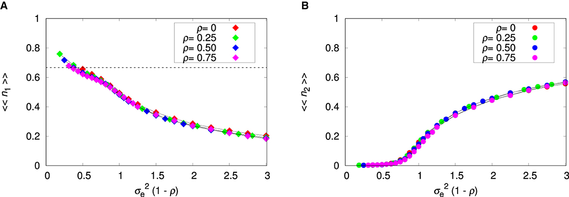
Figure 5. Influence of the variance of environmental values ${\sigma }_e^2$ and patch's environmental correlation ρ on the mean relative abundances. (A) Non-plastic species 1. (B) Plastic species 2. The parameters are L = 20, K_max = 100, c = 0, and p_mig = 0.3. The lines connecting the symbols are guides to the eye. The dashed horizontal line is 〈〈n₁〉〉 = 1/a₂₁ = 2/3.

Figure 6 shows the effect of migration on species coexistence for an uncorrelated landscape (ρ = 0). Increasing the migration probability p_mig has an effect similar to increasing the environment ruggedness. As pointed out in our study of the single-species dynamics, migration affects the adaptation of species 1 but has little to none influence on the adaptation of species 2 when phenotypic plasticity is non-costly. Hence, the increase of the abundance of species 2 with increasing p_mig shown in the figure is a result of the effect of migration on the abundance of species 1 which in turn affects species 2 in the ecological competition stage.

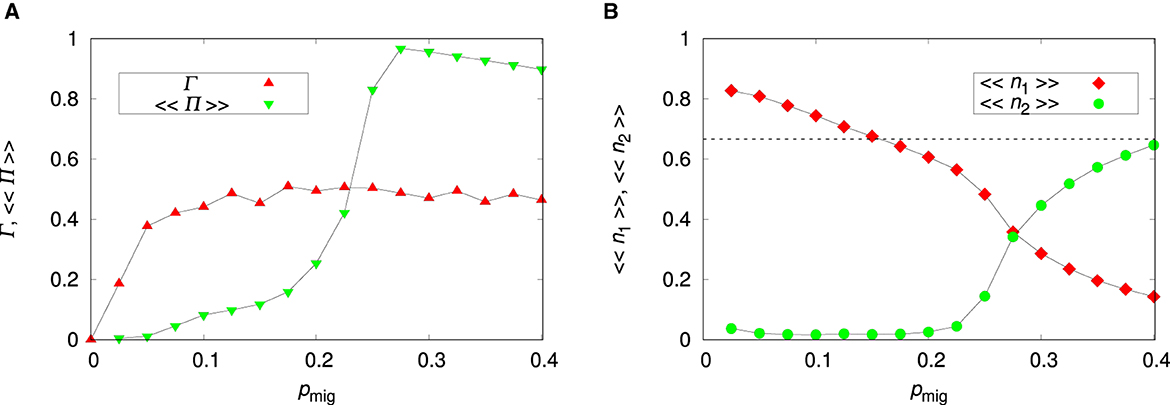
Figure 6. Influence of the migration probability p_mig on species coexistence for the uncorrelated environment. (A) Probability of coexistence Γ and probability of coexistence within a patch 〈〈Π〉〉. (B) Mean relative abundances of the non-plastic species 〈〈n₁〉〉 and of the plastic species 〈〈n₂〉〉. The parameters are L = 20, K_max = 100, c = 0, ${\sigma }_e^2=2$ and ρ = 0. The lines connecting the symbols are guides to the eye. The dashed horizontal line is 〈〈n₁〉〉 = 1/a₂₁ = 2/3.

The parameters ${\sigma }_e^2$, ρ and p_mig influence mainly the adaptation of the non-plastic species 1. The plasticity cost c, however, affects the plastic species 2 only and Figure 7 shows its effect on species coexistence. For the migration probability considered (p_mig = 0.3), species 1 cannot prevent invasion (and, consequently, coexistence) but for large c species 2 cannot take advantage of the maladaptation of species 1. We note that it is the presence of species 1 that drives species 2 to extinction, since species 2 alone can thrive for large c by turning off the plastic alleles (Figure 3). The data missing for c = 0.4 is because none of the runs resulted in coexistence.

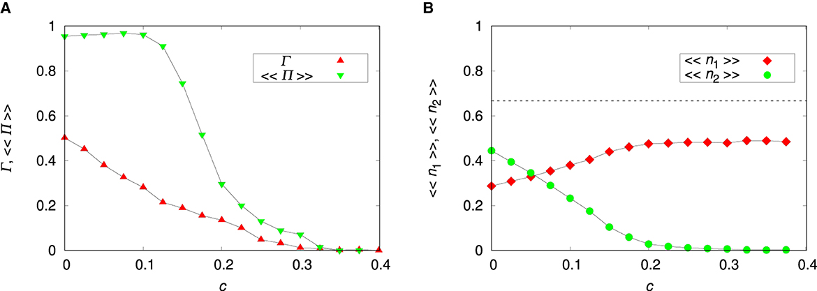
Figure 7. Influence of the plasticity cost c on species coexistence for the uncorrelated environment. (A) Probability of coexistence Γ and probability of coexistence within a patch 〈〈Π〉〉. (B) Mean relative abundances of the non-plastic species 〈〈n₁〉〉 and of the plastic species 〈〈n₂〉〉. The parameters are L = 20, K_max = 100, p_mig = 0.3, ${\sigma }_e^2=2$, and ρ = 0. The lines connecting the symbols are guides to the eye. The dashed horizontal line is 〈〈n₁〉〉 = 1/a₂₁ = 2/3.

3.2.1. Remarks on the simulation halting time, grid size, carrying capacity, and recombination

In our study, we assume that a running time of 2, 000 generations is sufficient to proclaim that the metapopulation dynamics reached equilibrium and hence that coexistence was achieved. Equilibrium population abundances are then evaluated by running the simulations for additional 100 generations when the relevant quantities are stored for averaging purposes. In Supplementary Figure 12, we show the time dependence of the relative abundances of both species for typical runs that led to coexistence. The results support our assumption that a halting time of 2, 000 generations is adequate to guarantee the equilibration of the metapopulation. Moreover, the dynamics reveals a most interesting feature of our model: the abundance of plastic species 2 increases much faster than its rival's in the initial generations, so species 2 rapidly colonizes almost the entire environment before it is partly or completely displaced by the non-plastic species 1 (see also Supplementary Figure 9).

Our analysis is restricted to a fixed grid size of linear length L = 20 and patch carrying capacity K_max = 100, which results in a very large carrying capacity for the metapopulation (viz., $L^2{K}_{max}=40,000$). Nevertheless, in the Supplementary material, we present the results for different choices of L and K_max. In particular, we show that there is practically no difference between the results for L = 15 and L = 20 (Supplementary Figures 13, 14), which indicates that our choice L = 20 for the linear dimension of the grid gives a good approximation to the limit of an infinitely large grid. The probability of coexistence Γ and the fraction of patches that harbor the two species 〈〈Π〉〉 increase with patch's carrying capacity K_max (Supplementary Figure 15), but the mean relative abundances of both species rapidly converge to their asymptotic values (Supplementary Figure 16), i.e., the values for K_max → ∞. Since in the case of costless plasticity it is the mean relative abundance of species 1 that determines whether within-patch coexistence can take place, these findings indicate that our choice of the grid size and patch carrying capacity probably describes very well the behavior of a very large population in a very large grid.

A limitation of our model is the assumption of asexual reproduction. Nearly all invasive species are sexual and, in the case of plants, highly selfing or clonal which is not the same as being strictly asexual. However, the simulations of asexual populations are much faster and easier to implement and reproduce than for the sexual populations, hence our option for that reproduction mode. In the Supplementary material, we offer some results for sexual species (Supplementary Figure 17). Recombination favors the non-plastic species 1 in the competition with the plastic species 2. In addition, for low and high mutation probabilities the sexual populations reach equilibrium faster than the asexual populations. But, as expected, the main conclusion of the paper is not affected by the reproduction mode: there is a regime of among-patch coexistence that happens for low migration probabilities that is due to the existence of patches that have too extreme environments for the non-plastic species, and a regime of within-patch coexistence that happens for intermediate migration probabilities, where the species coexist within most patches.

3.2.2. Simple argument for coexistence

Although our extensive simulations point rather unequivocally to the possibility of coexistence of the two species in a heterogeneous environment, here we offer analytical evidence for that finding. The aim is not only to dismiss suspicion that the observed coexistence is an artifact of our simulations but to complement the simulation results. Since the species at extinction risk—the plastic species 2—can thrive very well when alone in the patchy environment, the key to coexistence is the ecological competition stage (Section 2.3), so let us look at it more carefully.

First and foremost, we note that Equations (4a) and (4b) are not recursion equations. In fact, the quantities N_1i and N_2i that appear in their right-hand sides are the numbers of survivors of each species in patch i after viability selection, whereas the quantities $N_{1i}^{\prime }$ and $N_{2i}^{\prime }$ that appear in their left-hand sides are the numbers of offspring they bring forth. But only a fraction of these offspring will survive the selection sieve (and hence become adults) and this culling effect is not included in Equations (4a) and (4b). Let us assume that the metapopulation is at equilibrium (see, e.g., Supplementary Figure 12). The number of survivors of both species $N_{1i}^{eq}$ and $N_{2i}^{eq}$ at a given patch i must satisfy the condition

for the survival of species 2, and the condition

for the survival of species 1. These are necessary conditions for survival of each species in patch i as they ensure that the number of offspring will be greater than the number of survivors. (We recall that the number of survivors in a given generation is only a fraction of the number of offspring in the previous generation.) Inequality (6) can be rewritten as

which makes evident the impossibility of an equilibrium scenario where species 2 is present in patch i and $N_{1i}^{eq}/K_{max}>1/a_{21}$. Hence, increase of the entry a₂₁ decreases the chances of survival of species 2 and hence of coexistence. This is the reason we draw a line at 〈〈n₁〉〉 = 1/a₂₁ = 2/3 in the graphs for the relative abundance of species 1: the line delimits the regions where within-patch coexistence is possible. Note that a similar analysis for inequality (7) indicates that species 1 is extinct in patch i if $N_{2i}^{eq}/K_{max}>1/a_{12}=2$, a condition that is never satisfied in our simulations since N_2i and N_1i are less than K_max by construction. Therefore, within-patch coexistence is a possible outcome of the metapopulation dynamics, provided species 1 is locally maladapted in most patches, which is indeed the case for relatively large migration probabilities and environment variances.

However, Figure 7B exhibits a scenario where inequality (6) is satisfied and yet species 2 is extinct. Hence, condition (6) is necessary for survival of species 2, but it is not sufficient. In fact, a necessary and sufficient condition is that the production of offspring compensates the population decrease due to viability selection. For instance, assume that the number of offspring is twice the number of survivors, so condition (6) is satisfied, but that viability selection reduces the population to 1/4 of its size. Starting with 100 survivors, we get 200 offspring, then 50 survivors, then 100 offspring, then 25 survivors, and so on until extinction. This is the situation depicted in Figure 7B for high plasticity costs. A similar argument can explain the possibility of extinction of species 1 as well, despite the fact that inequality (7) is always satisfied. Unfortunately, we cannot express this necessary and sufficient condition in a simple mathematical formula because it involves the viability selection process and hence information on the individuals' phenotypes. This point highlights that to take advantage of the unfitness of species 1 in the rugged environment, species 2 must be well-adapted to it, hence the relevance of plasticity in our model.

Finally, we note that increase of the parameter r that governs the growth of both species in Equations (4a) and (4b) can be disastrous to species 2. The reason is that, other things being equal, $N_{1i}^{eq}$ increases with r so that the condition $N_{1i}^{eq}/K_{max}>1/a_{21}$ that prevents the growth of species 2 can be more easily fulfilled. Of course, the increase in the number of offspring of species 1 resulting from increasing r can be compensated by increasing the environment variance ${\sigma }_e^2$, which reduces their chances of survival.

4. Discussion

Our results challenge predictions from classical ecological theory by showing that a competitively superior species cannot always displace an inferior competitor in absence of niche differentiation and in a standard scenario of density- and frequency-independent viability selection. This conclusion obviously assumes that the ecologically inferior species 2 displays high levels of adaptive phenotypic plasticity (“any plasticity that allows individuals to have higher fitness in the new environment than it would were it not plastic”; Ghalambor et al., 2007, p. 396) and that plasticity can evolve quickly, which means that it harbors abundant genetic variation.

It has been conjectured that greater plasticity is a key mechanism underlying the success of invasive species (Baker, 1965), an idea that has some positive support in plants (Davidson et al., 2011) although there are counterexamples (Godoy et al., 2011). These inconsistent findings could be explained because adaptive plasticity might be a transient state during the invasion of new environments and thereafter disappear due to selection on the intersection of the reaction norm and eventual reduction of the slope, a process often referred to as “genetic assimilation” (Lande, 2009, 2015). The problem with this scenario is that for genetic assimilation to happen a very long time seems to be required if plasticity costs are low (Scheiner and Levis, 2021). In our case, with non-costly phenotypic plasticity the adaptation of species 2 during the colonization stage happens through phenotypic plasticity, i.e., the contribution of the rigid loci in Equation (2) to the adapted phenotype is negligible. In the Supplementary material, we test this scenario by assuming that no further migration takes place after the colonization period and find that genetic evolution remained largely irrelevant and no genetic assimilation was detected (see Supplementary Figure 4). The reason is that the increase in average fitness was very low to impose any selection on the intersection of the reaction norm (see Supplementary Figure 5). However, a different result is observed with costly plasticity, where adaptation after the colonization period results in a strong selective pressure to silence the contribution of the plastic alleles; i.e., genetic assimilation (see Supplementary Figure 6). In any case, whether or not an initial greater plasticity during the colonization process confers higher fitness is more contentious, though Davidson et al. (2011) consider that it is plausible.

Perhaps more controversial is the model's assumption that there is always plenty of genetic variation for plasticity so that populations will be able to adequately track the environment more closely. For instance, there seems to be limited ability for plasticity in thermal tolerance of ectotherms (over 90% of all animals), which should rely on behavioral thermoregulation to avoid overheating risk (Gunderson and Stillman, 2015; see also Sunday et al., 2014; Arnold et al., 2019). Although at spatial scales there is ample information on the genetic evolution of latitudinal clines for thermal-related traits (e.g., Hoffmann et al., 2002; Sgrò et al., 2010; Wallace et al., 2014; Castañeda et al., 2015), widely distributed Drosophila species do not seem to show higher plasticity for thermal tolerance than those from restricted areas, being their distributions more closely linked to species-specific differences in thermal tolerance limits (Overgaard et al., 2011). However, these conclusions are problematic because they were based on inferences that might grossly underestimate the population consequences of thermal plasticity. Thus, Rezende et al. (2020) have uncovered a dramatic effect of thermal acclimation in Drosophila, with warm-acclimated flies being able to increase the window for reproduction by nearly 1 month from mid-spring to early summer when compared with their cold-acclimated counterparts. In summary, answers to the important question of why adaptive plasticity is not more commonly observed should consider the heritability of plasticity (generally lower than trait heritability; Scheiner, 1993), the interactions among different traits (e.g., temperature-dependent trade-offs between fitness traits; Svensson et al., 2020), the reliability of habitat-specific cues (Tufto, 2000), and ecological constraints (Valladares et al., 2007; Scheiner, 2013; Snell-Rood and Ehlman, 2021).

We have focused in the situation where both species can simultaneously expand their range, which might not be an unrealistic scenario as range expansions have always occurred in the history of most species (Excoffier et al., 2009), and we are currently witnessing how species' range edges are expanding polewards in response to global warming (Mason et al., 2015). The important message here is that a successful invading species does not necessarily need to be ecologically superior to the resident one, it only needs to display some level of not much costly adaptive phenotypic plasticity under environmental conditions that usually vary across space and over time (Yeh and Price, 2004; Richards et al., 2006). Since empirical evidence indicates that costs of plasticity are infrequent or small (Murren et al., 2015), the former conclusion seems to be robust.

Finally, we can only speculate about the empirical relevance of our model. A recent empirical study reports that plasticity can enhance species coexistence by swiftly changing species' traits in response to a shift in the competitive environment, which was however assumed to be constant (Hess et al., 2022). It might be interesting to comment on Amarasekare's work on parasitoid coexistence in a spatially structured host–multiparasitoid community (Amarasekare, 2000a,b). The two parasitoid species she studied show asymmetric competition in the laboratory with one species being potentially capable of displacing the other, but both species can coexist in some metapopulations even though the two parasitoids have overlapping niches and compete for a shared limiting resource. She tested whether coexistence could happen via a trade-off between competitive ability and a higher dispersal of the inferior competitor, which could find patches where the superior competitor was absent. Her data showed that this was not the case, but pointed to local interactions as, e.g., density-dependent processes that could ameliorate antagonistic interactions in her study system. However, she did not estimate whether the fitness of egg parasitoids in the patches was differentially altered in the two species depending on the environmental conditions (e.g., temperature) at which individuals developed (Boivin, 2010). In other words, could phenotypic plasticity have played any role in explaining Amarasekare's findings? We do not know, but perhaps this is a hypothesis that has some merit.

Data availability statement

The original contributions presented in the study are included in the article/Supplementary material, further inquiries can be directed to the corresponding author.

Author contributions

JF and MS developed the concept of the study, were responsible for coding the simulations and model analyses (with input from MM), and wrote the original draft. MM revised the draft. All authors edited and revised the final draft. All authors contributed to the article and approved the submitted version.

Funding

JF was supported in part by Grant No. 2020/03041-3, Fundação de Amparo à Pesquisa do Estado de São Paulo (FAPESP) and by Grant No. 305620/2021-5, Conselho Nacional de Desenvolvimento Científico e Tecnológico (CNPq). MM was financed through the cE3c Unit FCT funding project UIDB/BIA/00329/2020. MS was funded by Grants PID2021-127107NB-I00 from Ministerio de Ciencia e Innovación (Spain), 2021 SGR 00526 from Generalitat de Catalunya, and the Distinguished Guest Scientists Fellowship Programme of the Hungarian Academy of Sciences (https://mta.hu).

Acknowledgments

This work benefited from discussions and insightful comments from Erol Akçay, Benjamin M. Bolker, Harold P. de Vladar, Eörs Szathmáry, Sam Scheiner, and Laurence Mueller.

Conflict of interest

The authors declare that the research was conducted in the absence of any commercial or financial relationships that could be construed as a potential conflict of interest.

Publisher's note

All claims expressed in this article are solely those of the authors and do not necessarily represent those of their affiliated organizations, or those of the publisher, the editors and the reviewers. Any product that may be evaluated in this article, or claim that may be made by its manufacturer, is not guaranteed or endorsed by the publisher.

Supplementary material

The Supplementary Material for this article can be found online at: https://www.frontiersin.org/articles/10.3389/fevo.2023.1077374/full#supplementary-material

References

Agrawal, A. A., Laforsch, C., and Tollrian, R. (1999). Transgenerational induction of defences in animals and plants. Nature 401, 60–63.
Amarasekare, P. (2000a). Coexistence of competing parasitoids on a patchily distributed host: local vs. spatial mechanisms. Ecology 81, 1286–1296. doi: 10.1890/0012-9658(2000)081[1286:COCPOA]2.0.CO;2
Amarasekare, P. (2000b). Spatial dynamics in a host-multiparasitoid community. J. Anim. Ecol. 69, 201–213. doi: 10.1046/j.1365-2656.2000.00378.x
Arnold, P. A., Nicotra, A. B., and Kruuk, L. E. (2019). Sparse evidence for selection on phenotypic plasticity in response to temperature. Philos. Trans. R. Soc. Lond. B Biol. Sci. 374, 20180185. doi: 10.1098/rstb.2018.0185
Baker, H. G. (1965). “Characteristics and modes of origin of weeds,” in The Genetics of Colonizing Species, eds G. L. Stebbins and H. G. Baker (New York, NY: Academic Press Inc.), 147–172.
Barabás, G., D'Andrea, R., and Stump, S. M. (2018). Chesson's coexistence theory. Ecol. Monogr. 88, 277–303. doi: 10.1002/ecm.1302
Boivin, G. (2010). Phenotypic plasticity and fitness in egg parasitoids. Neotrop. Entomol. 39, 457–463. doi: 10.1590/S1519-566X2010000400001
Bolnick, D. I., Amarasekare, P., Araújo, M. S., Bürger, R., Levine, J. M., Novak, M., et al. (2011). Why intraspecific trait variation matters in community ecology. Trends Ecol. Evol. 26, 183–192. doi: 10.1016/j.tree.2011.01.009
Bradshaw, A. D. (1965). Evolutionary significance of phenotypic plasticity in plants. Adv. Genet. 13, 115–155.
Calcagno, V., Mouquet, N., Jarne, P., and David, P. (2006). Coexistence in a metacommunity: the competition-colonization trade-off is not dead. Ecol. Lett. 9, 897–907. doi: 10.1111/j.1461-0248.2006.00930.x
Castañeda, L. E., Rezende, E. L., and Santos, M. (2015). Heat tolerance in drosophila subobscura along a latitudinal gradient: contrasting patterns between plastic and genetic responses. Evolution 69, 2721–2734. doi: 10.1111/evo.12757
Christiansen, F. B. (1975). Hard and soft selection in a subdivided population. Am. Nat. 109, 11–16.
Crow, J. F. (1958). Some possibilities for measuring selection intensities in man. Hum. Biol. 30, 1–13.
Davidson, A. M., Jennions, M., and Nicotra, A. B. (2011). Do invasive species show higher phenotypic plasticity than native species and, if so, is it adaptive? a meta-analysis. Ecol. Lett. 14, 419–431. doi: 10.1111/j.1461-0248.2011.01596.x
DeWitt, T. J., Sih, A., and Wilson, D. S. (1998). Costs and limits of phenotypic plasticity. Trends Ecol. Evol. 13, 77–81.
Doebeli, M. (1996). An explicit genetic model for ecological character displacement. Ecology 77, 510–520.
Excoffier, L., Foll, M., and Petit, R. J. (2009). Genetic consequences of range expansions. Annu. Rev. Ecol. Evol. Syst. 40, 481–501. doi: 10.1146/annurev.ecolsys.39.110707.173414
Fischer, B. B., Kwiatkowski, M., Ackermann, M., Krismer, J., Roffler, S., Suter, M. J. F., et al. (2014). Phenotypic plasticity influences the eco- evolutionary dynamics of a predator-prey system. Ecology 95, 3080–3092. doi: 10.1890/14-0116.1
Franco, C., and Fontanari, J. F. (2017). The spatial dynamics of ecosystem engineers. Math. Biosci. 292, 76–85. doi: 10.1016/j.mbs.2017.08.002
Franco, M., and Silvertown, J. (2004). Comparative demography of plants based upon elasticities of vital rates. Ecology 85, 531–538. doi: 10.1890/02-0651
Frazier, M. R., Huey, R. B., and Berrigan, D. (2006). Thermodynamics constrains the evolution of insect population growth rates: “warmer is better”. Am. Nat. 168, 512–520. doi: 10.1086/506977
Ghalambor, C. K., McKay, J. K., Carroll, S. P., and Reznick, D. N. (2007). Adaptive versus non-adaptive phenotypic plasticity and the potential for contemporary adaptation in new environments. Funct. Ecol. 21, 394–407. doi: 10.1111/j.1365-2435.2007.01283.x
Godfray, H. C. J., Cook, L. M., and Hasell, M. P. (1991). “Population dynamics, natural selection and chaos,” in Genes in Ecology, eds R. T. Berry, T. J. Crawford, and G. M. Hewitt (Oxford: Blackwell Scientific Publications), 55–86.
Godoy, O., Valladares, F., and Castro-Díez, P. (2011). Multispecies comparison reveals that invasive and native plants differ in their traits but not in their plasticity. Funct. Ecol. 25, 1248–1259. doi: 10.1111/j.1365-2435.2011.01886.x
Gómez-Llano, M., Germain, R. M., Kyogoku, D., McPeek, M. A., and Siepielski, A. M. (2021). When ecology fails: how reproductive interactions promote species coexistence. Trends Ecol. Evol. 36, 610–622. doi: 10.1016/j.tree.2021.03.003
Gomulkiewicz, R., and Kirkpatrick, M. (1992). Quantitative genetics and the evolution of reaction norms. Evolution 46, 390–411.
Gunderson, A. R., and Stillman, J. H. (2015). Plasticity in thermal tolerance has limited potential to buffer ectotherms from global warming. Proc. R. Soc. B 282, 20150401. doi: 10.1098/rspb.2015.0401
Hassell, M. P., Miramontes, O., Rohani, P., and May, R. M. (1995). Appropriate formulations for dispersal in spatially structured models: comments on bascompte and solé. J. Anim. Ecol. 64, 662–664.
Hastings, A. (1980). Disturbance, coexistence, history, and competition for space. Theor. Popul. Biol. 18, 363–373.
Hess, C., Levine, J. M., Turcotte, M. M., and Hart, S. P. (2022). Phenotypic plasticity promotes species coexistence. Nat. Ecol. Evol. 6, 1256–1261. doi: 10.1038/s41559-022-01826-8
Hoffmann, A. A., Anderson, A., and Hallas, R. (2002). Opposing clines for high and low temperature resistance in drosophila melanogaster. Ecol. Lett. 5, 614–618. doi: 10.1046/j.1461-0248.2002.00367.x
Kawecki, T. J., and Ebert, D. (2004). Conceptual issues in local adaptation. Ecol. Lett. 7, 1225–1241. doi: 10.1111/j.1461-0248.2004.00684.x
Kimura, M. (1965). A stochastic model concerning the maintenance of genetic variability in quantitative characters. Proc. Natl. Acad. Sci. U.S.A. 54, 731–736.
Lande, R. (2009). Adaptation to an extraordinary environment by evolution of phenotypic plasticity and genetic assimilation. J. Evol. Biol. 22, 1435–1446. doi: 10.1111/j.1420-9101.2009.01754.x
Lande, R. (2015). Evolution of phenotypic plasticity in colonizing species. Mol. Ecol. 24, 2038–2045. doi: 10.1111/mec.13037
Levins, R. (1969). Some demographic and genetic consequences of environmental heterogeneity for biological control. Bull. Entomol. Soc. Am. 15, 237–240.
Macarthur, R. H., and Levins, R. (1967). The limiting similarity, convergence, and divergence of coexisting species. Am. Nat. 101, 377–385.
Mason, S. C., Palmer, G., Fox, R., Gillings, S., Hill, J. K., Thomas, C. D., et al. (2015). Geographical range margins of many taxonomic groups continue to shift polewards. Biol. J. Linnean Soc. 115, 586–597. doi: 10.1111/bij.12574
Miller, M. B., and Bassler, B. L. (2001). Quorum sensing in bacteria. Annu. Rev. Microbiol. 55, 165–199. doi: 10.1146/annurev.micro.55.1.165
Murren, C. J., Auld, J. R., Callahan, H., Ghalambor, C. K., Handelsman, C. A., Heskel, M. A., et al. (2015). Constraints on the evolution of phenotypic plasticity: limits and costs of phenotype and plasticity. Heredity 115, 293–301. doi: 10.1038/hdy.2015.8
Muthukrishnan, R., Sullivan, L. L., Shaw, A. K., and Forester, J. D. (2020). Trait plasticity alters the range of possible coexistence conditions in a competition-colonisation trade-off. Ecol. Lett. 23, 791–799. doi: 10.1111/ele.13477
Nee, S., and May, R. M. (1992). Dynamics of metapopulations: habitat destruction and competitive coexistence. J. Anim. Ecol. 61, 37–40.
Overgaard, J., Kristensen, T. N., Mitchell, K. A., and Hoffmann, A. A. (2011). Thermal tolerance in widespread and tropical drosophila species: does phenotypic plasticity increase with latitude? Am. Nat. 178, S80–S96. doi: 10.1086/661780
Pásztor, L., Botta-Dukát, Z., Magyar, G., Czárán, T., and Meszéna, G. (2006). Theory-Based Ecology: A Darwinian Approach. Oxford: Oxford University Press.
Pérez-Ramos, I. M., Matías, L., Gómez-Aparicio, L., and Godoy, Ó. (2019). Functional traits and phenotypic plasticity modulate species coexistence across contrasting climatic conditions. Nat. Commun. 10, 2555. doi: 10.1038/s41467-019-10453-0
Pfennig, D. W. (2021). “Key questions about phenotypic plasticity,” in Phenotypic Plasticity and Evolution: Causes, Consequences, Controversies, ed D. W. Pfennig (Boca Raton, FL: CRC Press), 55–88.
Rezende, E. L., Bozinovic, F., Szilágyi, A., and Santos, M. (2020). Predicting temperature mortality and selection in natural drosophila populations. Science 369, 1242–1245. doi: 10.1126/science.aba9287
Richards, C. L., Bossdorf, O., Muth, N. Z., Gurevitch, J., and Pigliucci, M. (2006). Jack of all trades, master of some? On the role of phenotypic plasticity in plant invasions. Ecol. Lett. 9, 981–993. doi: 10.1111/j.1461-0248.2006.00950.x
Scheiner, S. M. (1993). Genetics and evolution of phenotypic plasticity. Annu. Rev. Ecol. Evol. Syst. 24, 35–68.
Scheiner, S. M. (1998). The genetics of phenotypic plasticity. VII. Evolution in a spatially-structured environment. J. Evol. Biol. 11, 303–320.
Scheiner, S. M. (2013). The genetics of phenotypic plasticity. XII. Temporal and spatial heterogeneity. Ecol. Evol. 3, 4596–4609. doi: 10.1002/ece3.792
Scheiner, S. M., Barfield, M., and Holt, R. D. (2020). The genetics of phenotypic plasticity. XVII. Response to climate change. Evol. Appl. 13, 388–399. doi: 10.1111/eva.12876
Scheiner, S. M., and Levis, N. A. (2021). “The loss of phenotypic plasticity via natural selection: genetic assimilation,” in Phenotypic Plasticity and Evolution: Causes, Consequences, Controversies, ed D. W. Pfennig (Boca Raton, FL: CRC Press), 161–181.
Schlichting, C. D. (1986). The evolution of phenotypic plasticity in plants. Annu. Rev. Ecol. Evol. Syst. 17, 667–693.
Schoener, T. W., and Spiller, D. A. (1987). High population persistence in a system with high turnover. Nature 330, 474–477.
Sgrò, C. M., Overgaard, J., Kristensen, T. N., Mitchell, K. A., Cockerell, F. E., and Hoffmann, A. A. (2010). A comprehensive assessment of geographic variation in heat tolerance and hardening capacity in populations of drosophila melanogaster from eastern australia. J. Evol. Biol. 23, 2484–2493. doi: 10.1111/j.1420-9101.2010.02110.x
Snell-Rood, E. C., and Ehlman, S. M. (2021). “Ecology and evolution of plasticity,” in Phenotypic Plasticity and Evolution: Causes, Consequences, Controversies, ed D. W. Pfennig (Boca Raton, FL: CRC Press), 139–160.
Sommer, R. J. (2020). Phenotypic plasticity: from theory and genetics to current and future challenges. Genetics 215, 1–13. doi: 10.1534/genetics.120.303163
Start, D. (2020). Phenotypic plasticity and community composition interactively shape trophic interactions. Oikos 129, 1163–1173. doi: 10.1111/oik.07194
Sunday, J. M., Bates, A. E., Kearney, M. R., Colwell, R. K., Dulvy, N. K., Longino, J. T., et al. (2014). Thermal-safety margins and the necessity of thermoregulatory behavior across latitude and elevation. Proc. Natl. Acad. Sci. U.S.A. 111, 5610–5615. doi: 10.1073/pnas.1316145111
Svensson, E. I., Gomez-Llano, M., and Waller, J. T. (2020). Selection on phenotypic plasticity favors thermal canalization. Proc. Natl. Acad. Sci. U.S.A. 117, 29767–29774. doi: 10.1073/pnas.2012454117
Tufto, J. (2000). The evolution of plasticity and nonplastic spatial and temporal adaptations in the presence of imperfect environmental cues. Am. Nat. 156, 121–130. doi: 10.1086/303381
Turcotte, M. M., and Levine, J. M. (2016). Phenotypic plasticity and species coexistence. Trends Ecol. Evol. 31, 803–813. doi: 10.1016/j.tree.2016.07.013
Uller, T. (2008). Developmental plasticity and the evolution of parental effects. Trends Ecol. Evol. 23, 432–438. doi: 10.1016/j.tree.2008.04.005
Valladares, F., Gianoli, E., and Gómez, J. M. (2007). Ecological limits to plant phenotypic plasticity. N. Phytol. 176, 749–763. doi: 10.1111/j.1469-8137.2007.02275.x
Via, S., and Lande, R. (1985). Genotype-environment interaction and the evolution of phenotypic plasticity. Evolution 39, 505–522.
Wallace, G. T., Kim, T. L., and Neufeld, C. J. (2014). Interpopulational variation in the cold tolerance of a broadly distributed marine copepod. Conserv. Physiol. 2, cou041. doi: 10.1093/conphys/cou041
Wasserman, L. (2004). All of Statistics: A Concise Course in Statistical Inference. New York, NY: Springer.
Keywords: adaptive plasticity, competitive interactions, eco-evolutionary dynamics, gene flow, spatial correlation
Citation: Fontanari JF, Matos M and Santos M (2023) Local adaptation, phenotypic plasticity, and species coexistence. Front. Ecol. Evol. 11:1077374. doi: 10.3389/fevo.2023.1077374
Received: 22 October 2022; Accepted: 26 April 2023;
Published: 15 May 2023.
Edited by:
Donald DeAngelis, United States Geological Survey (USGS), United States Department of the Interior, United StatesReviewed by:
Samuel Scheiner, National Science Foundation (NSF), United StatesLaurence Mueller, University of California, Irvine, United States
Copyright © 2023 Fontanari, Matos and Santos. This is an open-access article distributed under the terms of the Creative Commons Attribution License (CC BY). The use, distribution or reproduction in other forums is permitted, provided the original author(s) and the copyright owner(s) are credited and that the original publication in this journal is cited, in accordance with accepted academic practice. No use, distribution or reproduction is permitted which does not comply with these terms.
*Correspondence: Mauro Santos, mauro.santos@uab.es