Aerial abundance estimates for two sympatric dolphin species at a regional scale using distance sampling and density surface modeling

Introduction

Monitoring wildlife populations over scales relevant to management is a key challenge in conservation decision-making, particularly for species that occur at low densities across large geographic ranges. Coastal dolphins represent a key example of this challenge. Coastal dolphins provide a number of important ecosystem services (e.g., as top order predators of fish they store and transport nutrients and contaminants, regulate fish stocks through consumption and are prey themselves to other marine predators (Wells et al., 2004) and have high social and cultural value (Allen, 2014). In Australia, the three dolphin species present within coastal waters include the snubfin dolphin (Orcaella heinsohni), Australian humpback dolphin (Sousa sahulensis) (hereafter “humpback dolphin”) and Indo-Pacific bottlenose dolphin (Tursiops aduncus) (hereafter “bottlenose dolphin”), with the humpback and snubfin dolphins considered tropical species and the bottlenose dolphin present in both tropical and temperate habitats. The snubfin dolphin distribution is restricted to the Kimberley region in Western Australia, although vagrants are occasionally sighted at lower latitudes (Allen et al., 2012; Bouchet et al., 2021) whilst the distribution for both the bottlenose and humpback dolphins includes the lower latitudes of the Pilbara region in Western Australia. Therefore, this study focused on the latter two species rather than the former.

The humpback dolphin was uplisted from Data Deficient to Vulnerable in 2017 by the International Union for Conservation of Nature (IUCN), because of an inferred decline in abundance (International Union for Conservation of Nature, 2017), and is considered a threatened species across its estimated range, from Western Australia, across Northern Territory to Queensland and potentially southern New Guinea (Parra et al., 2017). Limited data on humpback dolphin abundance precludes population monitoring and in turn conservation assessments in Australia (Bejder et al., 2012). As such, the species remains a high priority for fundamental research in Western Australia (Waples and Raudino, 2018). There have been some efforts toward resolving this with estimates of population sizes at key sites across north western Australia, including the North West Cape in the Pilbara region (Brown et al., 2012; Hunt et al., 2017) and Cygnet Bay in the Kimberley region (Figure 1). Targeted photo-identification, vessel-based surveys have also been conducted off Onslow, in the Pilbara (Raudino et al., 2018a) and within Roebuck Bay, Beagle Bay, and Cone Bay in the Kimberley (Brown et al., 2016) however, abundance estimates were not possible for these sites due to low numbers of sightings and resighting rates. Limited gene flow detected between survey locations in Western Australia confirms that humpback dolphins are present as small, fragmented populations (Brown et al., 2014, 2017; Figure 1). Further, preliminary evidence of populations occurring in offshore areas associated with islands (e.g., Montebello Islands) indicates that the extent of the species’ distribution has yet to be fully mapped and it is not yet understood whether there is genetic connectivity between these dolphins and those using nearshore coastal waters of the Pilbara (Raudino et al., 2018b). Overall, their low density, uneven distribution (Hanf et al., 2022), and limited genetic connectivity across their range (Brown et al., 2014, 2017; Parra et al., 2018) make humpback dolphins particularly vulnerable to extinction (Parra et al., 2017).

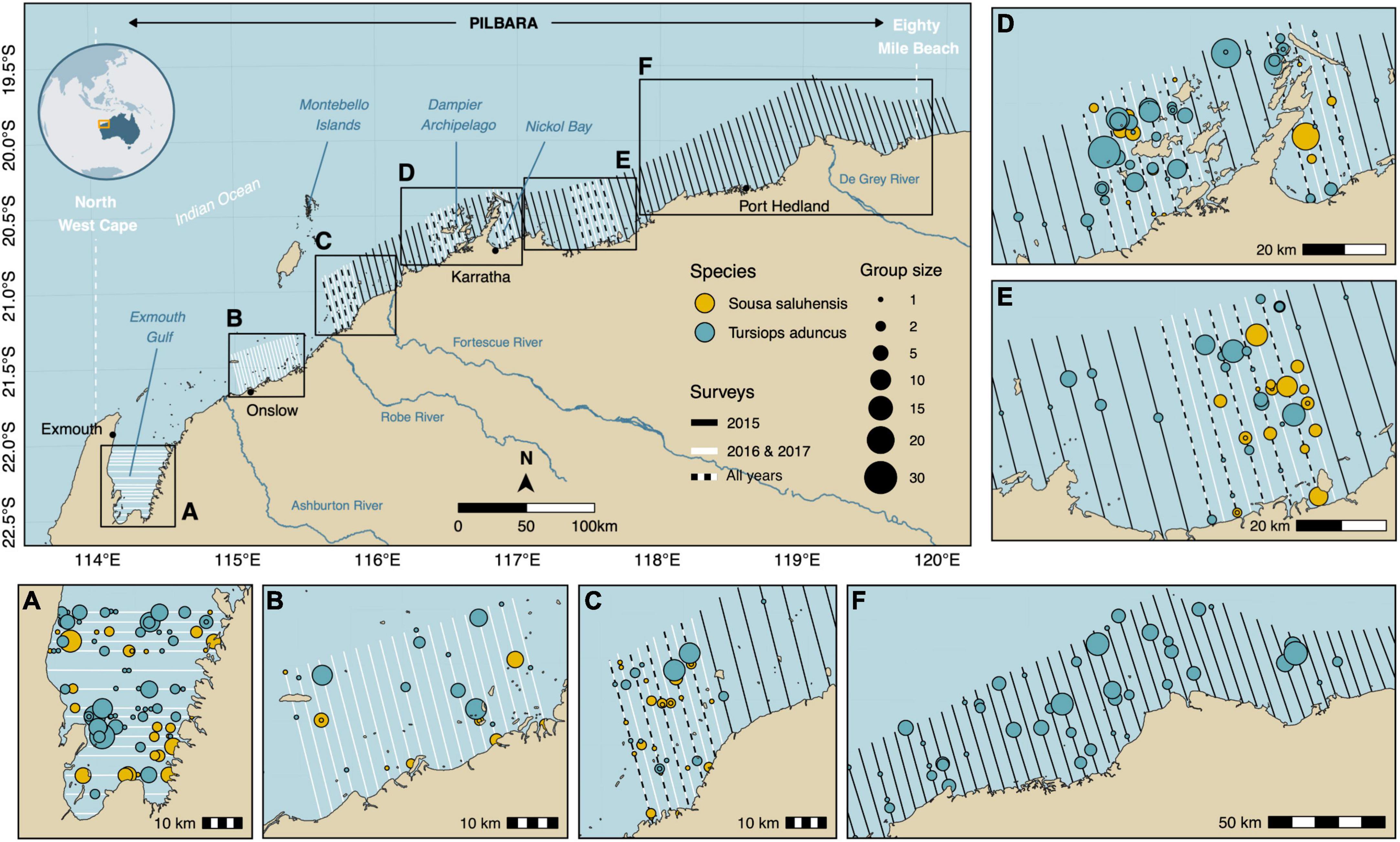
Figure 1. Map of the study area showing the location of transect lines for each survey time period. Detections of Australian humpback dolphins (Sousa saluhensis) and Indo-Pacific bottlenose dolphins (Tursiops aduncus) appear as filled circles in the map insets. (A) Exmouth Gulf, (B) Onslow and Thevenard Island, (C) Great Sandy Islands, (D) Karratha and Dampier Archipelago, (E) Balla Balla and (F) Port Hedland.

In comparison, the sympatric bottlenose dolphin has been demonstrated to be more abundant across the same area through several studies investigating its ecology, distribution and density patterns across the Pilbara (Preen et al., 1997; Allen et al., 2016; Raudino et al., 2018a; Haughey et al., 2020) and Kimberley regions (Brown et al., 2016). Despite having a wider distribution and being more abundant than the Vulnerable humpback dolphin, the species is also listed by the IUCN, as Near Threatened (Braulik et al., 2019) and a region-wide abundance estimate is not available for the Pilbara or Kimberley regions of Western Australia.

In Australia, threats across the ranges of humpback and bottlenose dolphins include habitat loss and degradation from coastal development, noise and water pollution, bycatch in trawl fisheries, disturbance and collisions with recreational and commercial vessels, prey depletion, and flooding, and other extreme events from climate change (Hale, 1997; Christiansen et al., 2010; Bilgmann et al., 2011; Meager and Limpus, 2014; Parra and Cagnazzi, 2016; Brooks et al., 2017; Braulik et al., 2019; Cagnazzi et al., 2020). In Western Australia, and particularly the Pilbara region, habitat loss and degradation are likely the major threats to dolphins using coastal waters and are associated with the construction of processing facilities and export infrastructure for petroleum and mineral industries. In addition, increased vessel traffic and noise associated with these industries has the potential to disturb and displace dolphins and increase the risks of vessel collisions that may result in mortalities or sub-lethal injuries (Parra and Cagnazzi, 2016). Furthermore, water quality is expected to decline in industrialized coastal areas and dolphins, being top order predators, are susceptible to the accumulation of high concentrations of harmful contaminants through bioaccumulation (Parra and Cagnazzi, 2016). Humpback dolphin populations in eastern Australia are already showing contaminant levels above thresholds where immunosuppression and reproductive anomalies occur, and levels comparable to those reported in other populations from highly industrialized countries (Cagnazzi et al., 2013). There are concerns over the cumulative impacts of current and future developments including multiple ports across the Pilbara region and expanding industry (Hanf et al., 2016).

The combination of a large geographic range and low density makes the Australian humpback dolphin a difficult species for which to estimate population size (Parra and Cagnazzi, 2016), particularly at a broad scale. With the exception of Corkeron et al. (1997), existing studies have surveyed humpback dolphins using vessels and estimated abundance using mark-recapture photo-identification techniques and replicate sampling of the same, relatively small areas (i.e., 100 s of km). This method has the advantage of yielding high resolution demographic data through sighting histories of individual dolphins (Lukoschek and Chilvers, 2008; Urian et al., 2015). However, this method can be resource intensive and ineffective for uncommon species with low numbers of sightings and re-sightings (Brooks et al., 2017) and is typically used for estimates over small areas.

While boat-based mark recapture is ideal for small study sites where the species of interest is abundant (i.e., bottlenose dolphins), aerial surveys using line transect sampling are preferable for estimating the abundance of marine mammals over broader areas such as at a region-wide scale. In particular, aerial surveys have been shown to be effective in estimating abundance of dolphin species that occur at low densities (e.g., Maui’s dolphins Cephalorhynchus hectori maui) (Slooten et al., 2006) and over large areas. Further, line transect data used in spatial modeling have the added advantage of providing information on non-homogonous distribution of individuals, highlighting biologically important areas that may be linked to environmental or ecological factors (Roberts et al., 2016). Such information is critical for enabling wildlife managers to prioritize on-going monitoring efforts and to manage overlap with pressures.

This study aimed to estimate the distribution of dolphins in the Pilbara, an area of data deficiency that is coming under increasing pressures from industry and climate change. We tested whether we could estimate the abundance of two morphologically similar tropical, coastal dolphin species, bottlenose and humpback dolphins, that occur sympatrically across this relatively large region by using aerial surveys with a distance sampling approach and used Density Surface Modeling (DSM) to investigate regional patterns of distribution.

Materials and methods

Study area

The Pilbara region spans 4,665 km of the northern Western Australian coast from the westerly point of North West Cape (21.8°S; 114.1°E) to the start of Eighty Mile Beach (19.9°S, 119.8°E) in the east. The Pilbara coastline is mainly open and exposed, with the exception of sheltered embayments in Exmouth Gulf, the Dampier Archipelago, and Nickol Bay. The region experiences two distinct seasons; a warm dry winter (June–September) with water temperature on average 20^°C across the region and a hot, wetter summer (October–April/May) with high water temperatures (20–30^°C). Coastal habitats are characterized by a number of large river systems carrying freshwater, mangroves and low-density ephemeral seagrass meadows, which may provide refuges for dolphin prey.

Data collection

We used a fixed high-wing aircraft (Partenavia P 68B) manned with observers for three aerial surveys conducted over 3 years: the first in May/June 2015, the second in May/June 2016, and the third in September 2017. The same survey methodology was used across all 3 years for all surveys. A maximum of two flights were flown per day (in the morning and in the afternoon), at least an hour after sunrise and an hour before sunset to optimize ambient light and thus viewing conditions. The middle of the day (survey stopped between 12:00–13:00) was avoided due to the incidence of glare on the ocean’s surface and to allow observers an opportunity to rest between flights when refueling of the aircraft took place. Flights were restricted to light wind conditions of less than 10 knots (18.5 km/h) a Beaufort sea state ≤3 to maximize detectability and limit the number of white caps visible on the water surface that could obscure animals and cause visual fatigue. If the weather conditions deteriorated during a flight, the survey was stopped and the remaining transects were postponed and flown at a later time in suitable conditions. Parallel transect lines were spaced 5 km apart, with each survey flight starting from a randomly selected transect and transects designed to extend offshore to the 20 isobath. The survey design included a total of 87 transects with a mean length of 40 km (SD: 7 km). The surveys were flown at 100 knots (185 km/h) ground speed and 500 ft (152 m) above sea level. These parameters were assumed constant during the survey as there were no data outputs from the speedometer or altimeter. The 500 ft (152 m) altitude was applied to the distance calculations during the analysis, despite some expected variation.

In 2015, we surveyed 24,038 km² (approximately half of the Pilbara region) along a continuous stretch of coast from Port Hedland to the Great Sandy Islands (Figure 1). Due to the low encounter rate of humpback dolphins in that year, the survey design was stratified in 2016 to focus on areas where the species was known to occur based on previous sightings. Survey effort was modified in those areas by increasing the number of transects and reducing the spacing between transects from 5 to 2.5 km (Figure 1), similar to Slooten et al. (2004). Additional habitats where humpback dolphins had been sighted incidentally during aerial surveys for dugong (Hodgson, 2007) or during boat-based surveys for humpback dolphins, were added to the flight plan in 2016 and 2017 and included the Montebello Islands (Raudino et al., 2018b) and Exmouth Gulf (Hunt et al., 2017; Figures 1, 3). In the latter region (19,943 km²), transect lines ran east-west rather than north-south to align with expected gradients in dolphin densities and reduce variance in encounter rates (Buckland et al., 2004; Thomas et al., 2010; Figures 1, 3). These dolphin species are indeed known to prefer shallow water habitats (7–10 m deep) (Raudino et al., 2018a; Haughey et al., 2021), which are found on the peripheral margins and southern part of the Gulf. Overall, the survey design included a total of 90 transect lines with a mean length of 38 km (SD: 8 km) in 2016 (Figure 1 and Supplementary Table 1). The 2016 design was followed in 2017, with the exception that Port Hedland and Montebello Islands were not covered due to unfavorable weather conditions and constraints related to aircraft maintenance. This reduced the number of transects in the 2017 survey to 72 with a mean length of 36 km and (SD: 8 km) (Figure 1 and Supplementary Table 1).

Surveys were led and conducted by a team of five experienced personnel, including four observers. The survey leader was positioned next to the pilot and recorded the middle-seat observations called and environmental data on glare angle with a protractor, turbidity (scored 1–4), and Beaufort sea state, as well as any changes in these during the survey (For more detail see Hodgson et al., 2013). Paired observers were positioned in the middle and rear seats and were both visually and acoustically isolated. Middle seat observers had considerable experience from previous marine fauna aerial surveys and rear seat observers generally had less experience but were at least qualified marine fauna scientists familiar with all species from vessel-based, if not aerial surveys. All observers participated in a training session prior to the survey to ensure they were familiar with the protocol. The aircraft was fitted with bubble windows for the middle seat observers and flat windows for the rear seat observers. The teams differed between years, and in 2017 only the port side was consistent throughout the survey, as the starboard observers were swapped at the midpoint in the survey. All observations were made with the naked eye, and were recorded into a voice-activated headset. Communication between observers was only made via an intercom when not on survey effort. This configuration maintained independence between observers, so that they were not cued of sightings made by one another. When a dolphin group was detected, the observer would state their identity, the species, their certainty of species identification, the declination angle (measured with a Suunto clinometer PM-5) to the group when abeam, their best estimate of group size, a minimum and maximum group size range, including a separate count of calves if present, and a score for water turbidity on a discrete scale of categories 1–4 (see Hodgson et al., 2013). Sightings by the paired middle seat and rear seat observers were considered the same if the time stamp from the audio transcription i.e., the call by the rear-seat observer (re-capture) was within 10 s of the front-seat observer and if the position of the dolphin group relative to the transect (indicated by both declination angles) and the group size called were comparable (Raudino et al., 2022). The survey was mostly flown in passing mode, whereby transects are followed without deviating and observers record observations from the transect line (Caughley, 1974). However, the aircraft was allowed to leave the transect line and circle a dolphin group (i.e., enter closing mode) (Strindberg and Buckland, 2004) to better estimate the size of dolphin groups comprising >5 individuals and to confirm species identity. Closing mode approaches did not last more than ∼5 min for each group sighting; following this, the aircraft rejoined the transect line at the point where it departed from it. Wing-mounted cameras were also used to confirm species identification, where the camera field of view overlapped the field of view of the observers (Raudino et al., 2022). Observers simultaneously recorded sightings of other marine taxa such as cetaceans, dugong, turtles, and large sharks and rays Hodgson et al. (2013). The middle seat observations recorded by the survey leader were checked post-field and recordings from the rear two observers were transcribed once back on the ground using the software Audacity. Flight path co-ordinates were logged automatically every 2 s by two separate GPS units and the location for each second was estimated by taking the average of the location before and after. The times from the GPS were then matched to the audio recordings.

Density surface modeling

We built density surface models (DSMs) for both humpback and bottlenose dolphins separately. DSMs are spatially explicit models of wildlife abundance that have been corrected for uncertain detectability using conventional distance sampling methods (Hedley and Buckland, 2004; Thomas et al., 2010; Miller et al., 2013), and are advantageous as they (i) relax some of the assumptions of design-based methods, allowing the analysis of non-systematic data (e.g., from platforms of opportunity), (ii) can reduce uncertainty in estimates of abundance by explicitly capturing between-transect variance, (iii) allow insights into the ecology of focal species by linking counts to biotic and/or abiotic covariates such as depth, distance from coast, or spatial coordinates (i.e., latitude and longitude) (Miller et al., 2013). It is important to note that our focus was on abundance estimation rather than species-habitat relationships. DSMs are increasingly being applied to estimate cetacean abundance (Williams et al., 2011; Hammond et al., 2013; Best et al., 2015; Dellabianca et al., 2016; Roberts et al., 2016; Kanaji et al., 2017; Sigourney et al., 2020). The advantage of this technique lies in being able to understand and visualize the spatial distribution of abundance. This is particularly important for species that do not have a homogenous distribution across their range and may only inhabit a relatively small area.

Density surface models are built using a two-stage approach: first, a detection function is fitted to the observations to quantify the proportion of animals detected within contiguous segments of the transect lines; second, estimates of animal abundance within individual segments are modeled as smooth functions of explanatory covariates within a generalized additive model (GAM) framework (Thomas et al., 2010; Miller et al., 2013). Most studies divide transects into segments of approximately equal length (i.e., twice the right-truncation distance, which usually falls between 0.5 and 25 km), so that segments remain sufficiently small that neither animal density nor habitat conditions vary appreciably within them (Miller et al., 2013). However, this can pose problems in (i) aerial surveys where the geographic extent of sampling coverage is several orders of magnitude larger than truncation distances, resulting in numerous (potentially empty) segments, and (ii) remote, data-deficient areas where habitat features are only mapped at coarse resolution, leading to many segments with very similar covariate values. Following guidelines for best practice, we therefore performed a sensitivity analysis to assess the influence of segment length on model inference (Roberts et al., 2021). We used segments of 2.5 and 5 km in length, which are commensurate with the range of sizes used in previous dolphin studies (Williams et al., 2011; Becker et al., 2014; Dellabianca et al., 2016), and found no appreciable differences in DSM predictions, fit, or residual diagnostics between the two (data not shown). Given this and the low apparent density of humpback dolphins in the area, we opted for a segment length of 5 km to maximize the number of segments with positive counts.

Detection function

We fitted species-specific detection functions using the multiple-covariate distance sampling (MCDS) engine available in the Distance package for R version 4.0.3 (Buckland et al., 2001; Marques and Buckland, 2004; Miller, 2012; Miller et al., 2019). As all surveys were conducted from the same observation platform and followed identical protocols, we pooled data across all years to obtain sufficient sightings for model fitting and to produce a detection function per species. Perpendicular distances (d) to animal groups were calculated as d = h*tan [Rad(90-α)], where h is the survey altitude (152 m) and α the declination angle to a sighting when abeam (Lerczak and Hobbs, 1998; Bröker et al., 2019). Distances were left-truncated at 100 m to account for obstructions to the field of view by parts of the aircraft, as well as the difference in field of view between observers due to the bubble windows (middle) and flat windows (rear) and to account for the difference in height of the observers. The maximum declination angles were compared between observers and a decision was made to left truncate accordingly. All distances had 100 m subtracted, so that points at 100 m from the trackline correspond to distance zero in the analysis (Borchers et al., 2006; Salgado Kent et al., 2012). We also right-truncated the humpback dolphin data at 450 m; this distance corresponds to an average sighting window of 7 s, which matches the conditions used to derive the only availability bias correction factor in existence for Australian humpback dolphin (Brown et al., 2022)—assuming a lateral field of view defined as a circular sector with a central angle of 100^° (Forcada et al., 2004). Doing so removed a small proportion (4.7%) of the furthest sightings, which is acceptable given that these contribute little to the estimation (Buckland et al., 2001; Thomas et al., 2010). In contrast, we did not right-truncate the bottlenose dolphin data, as availability bias correction factors for Indo-pacific bottlenose dolphin are based on much longer sighting windows (ca. 15–30 s) that are achieved beyond the largest distances recorded for the species in our surveys. We considered both half-normal and hazard-rate key functions (without adjustment terms) and tested several candidate model formulations, including different combinations of single covariates (i.e., Beaufort sea state and group size), in addition to perpendicular distance alone. Models were ranked on the basis of their Akaike’s Information Criterion (AIC) scores, and models within ≤2 AIC units of each other were considered to be equally supported (Mannocci et al., 2017a), conditional on satisfying goodness-of-fit tests. A Horvitz-Thompson-like estimator of the total number of individuals in segment j, ${\widehat{N}}_j$, within the covered area is given by:

Where R_j is the total number of observed groups in segment j, s_jrdenotes the size of the r^th group in segment j, and $\widehat{p}({\mathbf{\text{z}}}_{jr})$ represents the estimated probability of detection given observation-level covariate z_jr (Marques et al., 2007).

Hierarchical GAM

Due to differences in survey designs between years as well as there being too few humpback dolphin sightings in 2015 to model abundance, we treated the 2015 bottlenose dolphin data separately. For the period 2016–2017, we hypothesized that each dolphin species would exhibit a stable underlying distribution pattern, from which annual deviations would occur. We therefore modeled the estimated dolphin abundance in segment j within transect k using a hierarchical GAM (Model GI, sensu Pedersen et al., 2019) of the general form:

where ${\widehat{N}}_{jk}$ follows a Tweedie distribution, as is common in the analysis of cetacean survey data (Miller et al., 2013; Roberts et al., 2016; Sigourney et al., 2020). Note that the Tweedie distribution is equivalent to the distribution obtained by summing a Poisson number of gamma random variables (i.e., a compound Poisson/Gamma distribution), and is therefore particularly useful to account for over-dispersion and zero-inflation (Foster and Bravington, 2013). β₀ is an intercept, f(z_j) is a global bivariate smooth of longitude and latitude (shared between years), f_year(z_j) is a year-specific trend that accounts for deviations from the global trend, and b_k is a random effect term to account for similarities in counts between adjacent segments within the same transect line k and accommodates correlated observations due to repeat coverage of the same transects in some years. The latter improved model fit. As per Becker et al. (2022), effort was accounted for via a single offset term given by the product of a correction factor for detectability on the trackline (${\widehat{g}}_{(0)}^{\prime }$, see below) and the area a_j of segment j, calculated as:

Where w_R is the right-truncation distance, and l_J is the segment length. Conventional bivariate spatial splines may perform poorly in the presence of physical boundary features such as the numerous islands and peninsulae found along the Pilbara coastline (Wood et al., 2008; Scott-Hayward et al., 2014). We therefore parameterised f as soap film smooths, which are appropriate for finite area smoothing within complex spatial domains (Miller and Wood, 2014). Year-level smoothers were fit using low-order penalized derivatives (m = 1 in the mgcv package) to reduce collinearity between them and the global smoother (Pedersen et al., 2019). Following Mannocci et al. (2017b), we used restricted maximum likelihood (REML) as the estimation criterion because it penalizes over-fitting and leads to more pronounced optima (Wood, 2011). Abundance estimates were obtained by summing marginal model predictions over all cells (ca. 18 km²) within a spatially referenced hexagonal grid spanning the study area. Estimates of uncertainty were obtained via the Delta method [as implemented in the R package (“dsm”) dsm.var.gam function], which assumes independence between the detection function and the spatial process (Bravington et al., 2021). To visualize uncertainty in abundance predictions, we computed the coefficient of variation for each prediction grid cell and plotted these as a map of the region (Winiarski et al., 2014).

Visibility bias correction

Line transect methods assume that detection on the survey trackline is certain [i.e., g(0) = 1], but this is seldom the case in aerial surveys of diving marine mammals, as individuals may be either submerged and not visible or within view but missed by observers (e.g., due to cloud cover, sea state, or observer fatigue) (Laake et al., 1997). Marsh and Sinclair (1989) coined the terms “availability” and “perception” bias to, respectively differentiate between these two sources of errors, both of which can lead to underestimating abundance if ignored (Barlow, 1999). Availability bias is problematic for coastal dolphins due to the high speed of travel of the aircraft relative to the typical duration of the animals’ surfacing intervals within the course of an overhead pass (Slooten et al., 2004). Furthermore, studies have shown that availability bias can vary across species (Palka, 2020), seasons (Durden et al., 2017) environmental conditions (e.g., turbidity), and group sizes (Gómez De Segura et al., 2006; Durden et al., 2017; Sucunza et al., 2018). To our knowledge, no estimates of availability bias ($\widehat{a}$) currently exist for bottlenose dolphins in our area. We therefore took the average of published values for common bottlenose dolphin (Tursiops truncatus), a related species, in similar environments (i.e., Tursiops = 0.68, Forcada et al., 2004; 0.8, Durden et al., 2011; 0.78, Lauriano et al., 2014). Recent unmanned aerial vehicle (i.e., drone) surveys suggest a group-size corrected mean availability of ${\widehat{a}}_{sousa}$ = 0.48 for humpback dolphins in Australia (Brown et al., 2022).

We evaluated perception bias by analyzing the joint and conditional detection histories of both front and rear observers in a logistic regression framework, as implemented in the mark-recapture distance sampling (mrds) package (Burt et al., 2014; Laake et al., 2021). This required the identification of duplicate sightings based on coincidence in timing (see Raudino et al., 2022 for more detail). We used an independent observer configuration, in which detections by each observer serve as a set of binary trials for the other, with the outcome either a “success” when both observers detect the same animals or a “failure” otherwise. This configuration is useful when animals are unlikely to have moved in response to the survey platform between detection by each observer (Burt et al., 2014). Even if observers are not directly cued by one another, unmodeled heterogeneity in detection probability (i.e., the preferential detection of the “most observable” animals) can still compromise independence and induce bias in abundance estimates (Laake et al., 2011; Rankin et al., 2020). Because of this, we built Mark Recapture Distance Sampling (MRDS) models with different combinations of covariates (i.e., group size, turbidity, and Beaufort sea state, in addition to distance) and compared them using AIC. We tested a half normal key function under both full (FI) and point (PI) independence assumptions, whereby detections are, respectively taken to be independent at all distances (i.e., no unmodeled heterogeneity) or at perpendicular distance zero only (Borchers et al., 2006; Burt et al., 2014). In both cases, a binomial generalized linear model is fitted to the double observer data to estimate the form of the conditional detection functions, p(y), which give the probability that a dolphin group located at distance y is seen by observer 1 given it was seen by observer 2, or vice versa (Rankin et al., 2020). A distance sampling model is also fitted to the observed distances of all detected groups to estimate the relative detection function, g(y). In an FI model, p(y) is taken to be an unbiased estimator of the detection probability d(y), such that p(y)=d(y). In contrast, PI models use the mark-recapture component only to estimate the probability of detection on the transects, giving $d\left(y\right)={\widehat{p}}_{(0)}g(y)$ (Burt et al., 2014; Rankin et al., 2020). The average perception bias across years was ${\widehat{p}}_{(0)}$ = 0.899 (± 0.062 SD, n = 3) for bottlenose dolphins and ${\widehat{p}}_{(0)}$ = 0.931 (± 0.093, n = 2) for humpback dolphins. An overall correction factor for detectability was obtained by multiplying availability and perception bias estimates: ${\widehat{g}}_{(0)}^{\prime }={\widehat{p}}_{(0)}\widehat{a}$ (Wood, 2017).

All R code used for the analysis is available on GitHub at https://github.com/pjbouchet/sousa_dsm.

Results

Aerial surveys conducted between 2015 and 2017 yielded a total of n = 341 dolphin detections (n = 336 after right-truncation), including 235 groups of bottlenose dolphins and 106 groups of humpback dolphins (Supplementary Table 1). Transect lines spanned a cumulative distance of 9,810 km, representing 2,085 segments (Supplementary Table 1). Bottlenose and humpback dolphins were encountered on ca. 8% (n = 173) and ca. 4% (n = 88) of these segments, respectively. Sightings largely consisted of small groups of 1–4 individuals (bottlenose: n = 187, ca. 80%; humpback: n = 91, ca. 86%). The largest recorded groups comprised 27 bottlenose and 23 humpback dolphins, respectively. Most sightings for both species occurred in Exmouth Gulf (Figure 1; Inset A), Sandy Islands (Figure 1; Inset C), Dampier Archipelago (Figure 1; inset D), and near Balla Balla (Figure 1; Inset E).

Detection function

The detection function model was not sensitive to the choice of key function, with the half-normal and the hazard rate functions largely receiving equal statistical support for each species based on the AIC (Supplementary Table 2). However, models with group size as a covariate were selected to account for differences in the detectability of smaller and larger dolphin groups (Figure 2). We present results from a half-normal model here, but the hazard rate yielded comparable abundance estimates (Supplementary Table 3). The inclusion of Beaufort sea state did not improve model fit, so this covariate was not considered further. Average detection probabilities were 0.51 (± 0.03 SE) and 0.55 (± 0.04 SE) for bottlenose and humpback dolphins, respectively (Figure 2).

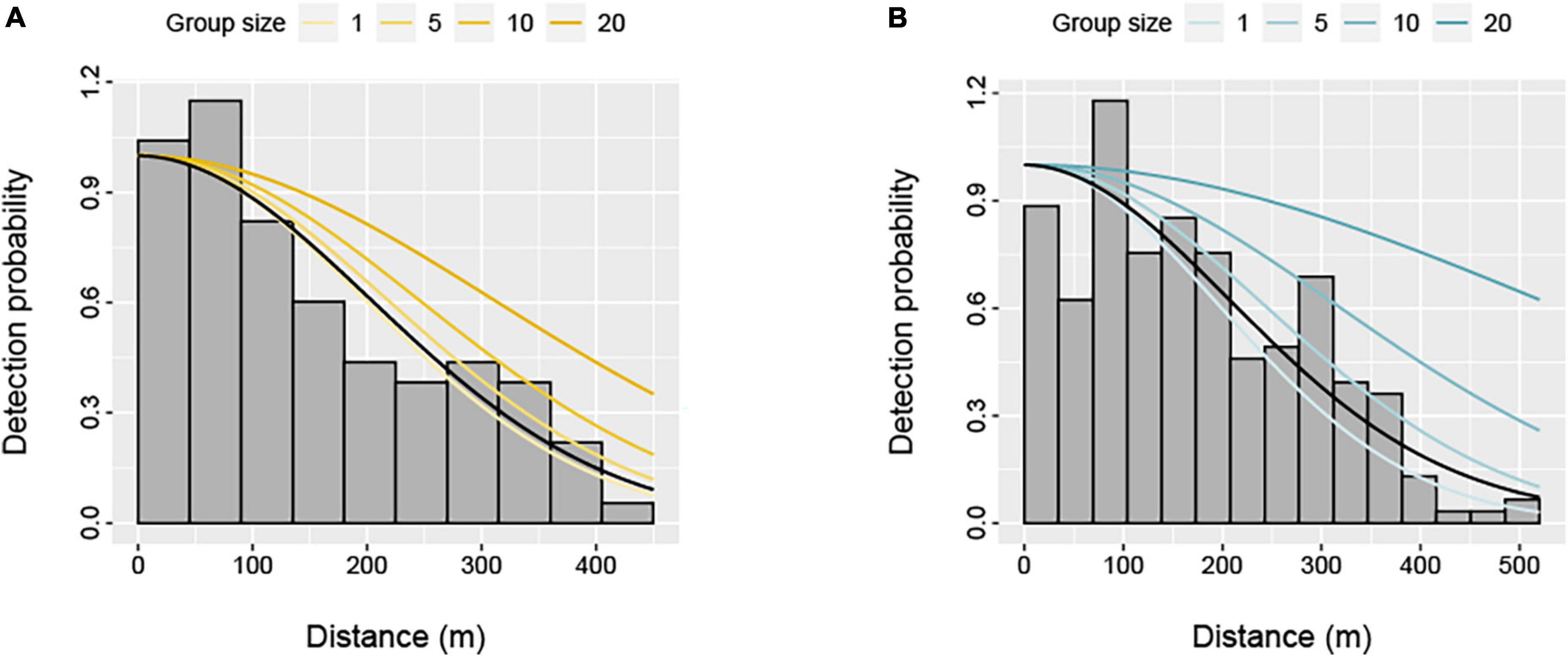
Figure 2. Distribution of perpendicular detection distances for (A) humpback dolphins (Sousa saluhensis) and (B) bottlenose dolphins (Tursiops aduncus) during aerial surveys of the Pilbara region. Fitted half-normal detection functions for selected dolphin group sizes (included as a covariate) are shown as solid lines. The black line represents the average detection function.

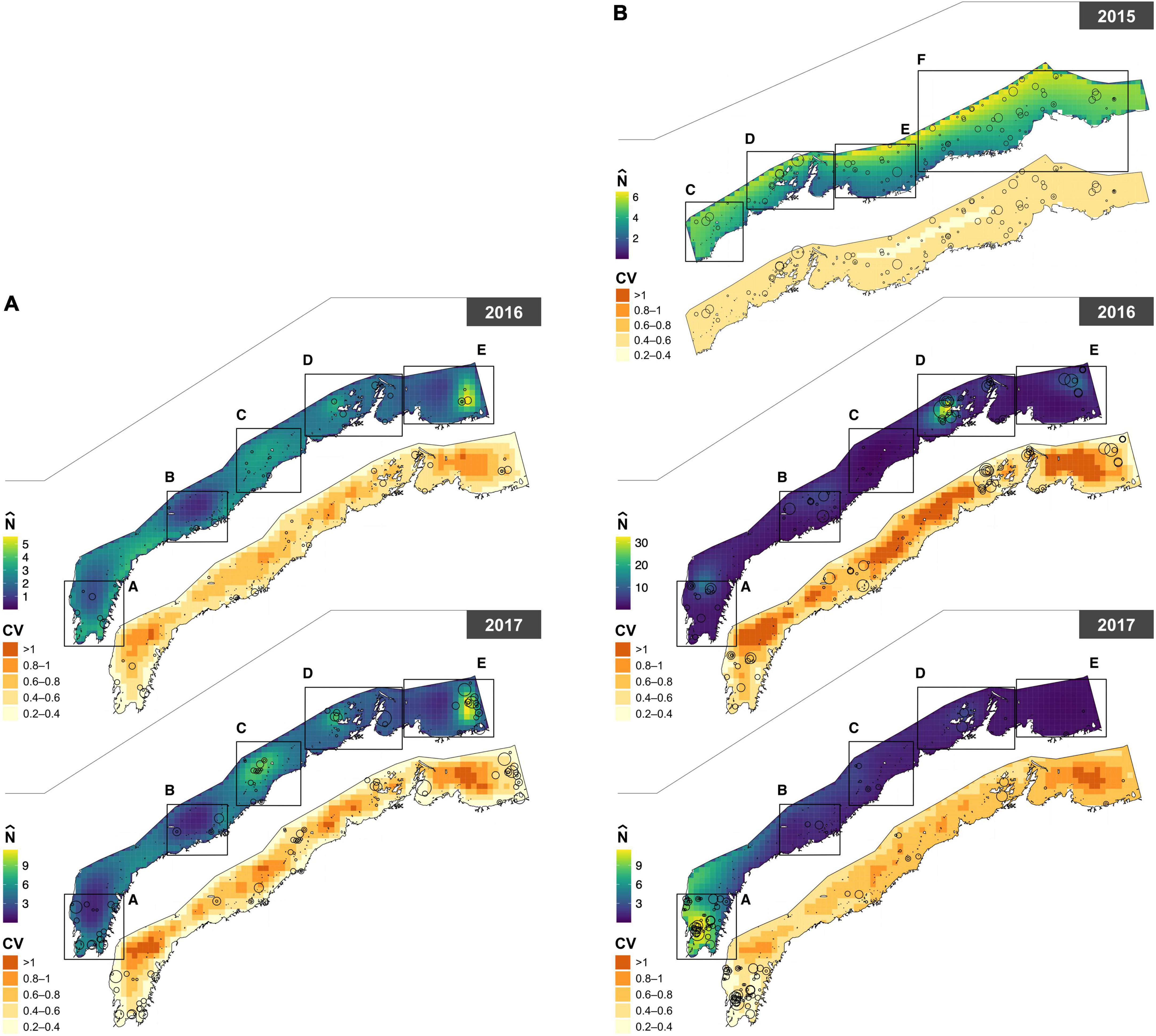
Figure 3. Paired maps of predicted abundance ($\widehat{N}$) for (A) humpback (Sousa saluhensis) and (B) bottlenose (Tursiops aduncus) dolphins, with associated uncertainty (represented as the coefficient of variation, CV). Circles represent sightings of dolphin groups; their size is proportional to group size (see Figure 1 for details).

Density surface modeling

A Tweedie distribution with a log link function for the response provided a good fit to the data, with no appreciable departures from residual assumptions (Supplementary Figure 1). The DSM predicted the highest densities of dolphins of both species closest to the coast with the exception of 2015.

The power parameter of the Tweedie was estimated as p = 1.32 in the 2015 bottlenose dolphin model, p = 1.32 in 2016–2017 bottlenose dolphin model, and p = 1.25 in the humpback dolphin model. The DSMs explained 16.2% (bottlenose, 2015), 27.3% (bottlenose, 2016–2017), and 16.1% (humpback, 2016–2017) of the deviance, and predicted that the densities of both species were highest close to the coast in all years except 2015, when bottlenose dolphin abundance peaked in offshore waters. In 2016–2017, bottlenose dolphins were predicted to be more abundant around the Dampier Archipelago and in Exmouth Gulf. Humpback dolphin abundance was more uniform across the study area in 2016 than 2017, but more concentrated around the Great Sandy Islands, Dampier Archipelago, and Balla Balla in 2017 (Figure 3). The estimated abundance of bottlenose dolphins in the 2015 survey area (24,038 km²) was 3,713 (95% CI = 2,679–5,146; CV = 0.17). Note the study area size and effort does differ between years and this should be taken into account when interpreting these results (Supplementary Table 1). Abundance estimates for bottlenose dolphins in 2016 and 2017 were 2,638 (95% CI = 1,670–4,168; CV = 0.24) and 1,635 (95% CI: 1,031–2,593; CV = 0.24), respectively, in a study area of (19,943 km²). This corresponds to an average density (across grid cells) of 0.189 (± 0.046 SD) bottlenose dolphins per km² in 2015, 0.159 (± 0.135 SD) in 2016, and 0.101 (± 0.103 SD) in 2017. The estimated abundance of humpback dolphins in 2016 and 2017 was 1,546 (95% CI = 942–2,537; CV = 0.26) and 2,690 (95% CI: 1,792–4,038; CV = 0.24), respectively. This corresponds to an average density of 0.097 (± 0.03 SD) humpback dolphins per km² in 2016 and 0.169 (± 0.064 SD) in 2017. These estimates were corrected for visibility bias using ${\widehat{g}}_{(0)}^{\prime }$ = 0.665 for bottlenose dolphins and ${\widehat{g}}_{(0)}^{\prime }$ = 0.447 for humpback dolphins. A comparative analysis of the 2015 data using Conventional Distance Sampling (CDS) and MRDS yielded similar results (see Supplementary material). Uncertainty in spatial predictions was highest along the middle band and the eastern extent of the study area (Figure 3).

Discussion

This study presents the first abundance estimates for bottlenose and humpback dolphins at a regional scale in Western Australia across multiple years. At this broad scale, the abundance of each dolphin species varied both spatially and temporally. Dolphin abundance was noticeably higher in Exmouth Gulf (extending into North West Cape) and Dampier Archipelago for both species across multiple survey years (Figure 3). These findings corroborate the relatively high abundance estimates that have been reported in vessel based mark-recapture photo identification studies within the smaller and localized study areas of North West Cape and Exmouth Gulf for both bottlenose (Haughey et al., 2020) and humpback dolphins (Brown et al., 2012; Hunt et al., 2017; Sprogis and Parra, 2022) and inferred for humpback dolphins in Dampier Archipelago (Allen et al., 2012). Similar results have been reported by Hanf et al. (2022) who modeled the distribution of these species based on aerial survey data from the western Pilbara. In contrast, the coastal waters between the northern end of Exmouth Gulf and Dampier Archipelago, generally had lower dolphin abundance, consistent with findings from boat-based mark recapture surveys undertaken in 2015 and 2016 in this area (Raudino et al., 2018a). Collectively, these findings confirm the non-homogonous nature of dolphin distribution and we suspect that environmental or other biotic variables are potentially influencing this distribution i.e., prey distribution, SST etc.

It is worth noting that the modeled distribution of bottlenose dolphins was predominantly further offshore in 2015 than in subsequent years (2016 and 2017). This apparent shift coincided with the only El Niño event that occurred during the study period. El Niño events are known to affect the strength of the coastal Leeuwin current off Western Australia. Sprogis et al. (2018) found that El Niño events are linked with a negative anomaly in sea surface temperature (SST) and above average rainfall which likely influences the distribution of dolphin prey, resulting in a temporary change in abundance and distribution as reported for bottlenose dolphins in south western Australia (Sprogis et al., 2018), and other cetacean species [e.g., Gray whales (Eschrichtius robustus) Gardner and Chávez-Rosales, 2000]. Hanf et al. (2022) also found that SST and El Niño influenced the distribution of bottlenose dolphins to offshore waters, consistent with this study. Nevertheless, this offshore distribution may be anomalous given other studies have shown there was a higher probability of bottlenose dolphins using coastal waters in this area at this time of year (Haughey et al., 2021).

Previous abundance estimates of humpback dolphins at specific study sites across Australia have been relatively low, ranging from 14 to 207 individuals per site with most populations studied estimated to be <100 mature individuals, though within areas much smaller than the present study (100–1000 km²) (Corkeron et al., 1997; Parra et al., 2006; Cagnazzi et al., 2011; Brown et al., 2016; Parra and Cagnazzi, 2016; Brooks et al., 2017; Raudino et al., 2018a,b). One of the highest densities of humpback dolphins previously reported is for North West Cape (which overlaps with our study area), where Hunt et al. (2017) estimated a population of 129 individuals in a 130 km² area (i.e., nearly one humpback dolphin per km²) compared to our average density of 0.097 (± 0.03 SD) per km² in 2016 and 0.169 (± 0.064 SD) in 2017. This is an order of magnitude larger than the density estimates we obtained for the Pilbara. Conversely, bottlenose dolphins across tropical Australia have been found to be more abundant than humpback dolphins across similar habitats (Chilvers and Corkeron, 2003; Brown et al., 2016; Raudino et al., 2018a; Haughey et al., 2020), with the exception of the Northern Territory where humpback dolphins are more prevalent (Palmer et al., 2014; Brooks et al., 2017). This may be a reflection of niche partitioning and exploiting different habitat or prey, as has been documented within dolphin populations elsewhere (Kiszka et al., 2012; Ansmann et al., 2015) and between sympatric tropical dolphin species in other studies in Australia (Parra, 2006; Haughey et al., 2021). Importantly, both species are noted to occur in small local populations with variable genetic connectivity across north Western Australia (Brown et al., 2014; Allen et al., 2016; Brown et al., 2017).

Challenges of studying dolphins at a regional scale

These findings of low abundance and uneven density in their distribution have clear implications for the conservation of two iconic coastal cetaceans across their range, including within the Pilbara region. For instance, our study confirms low, yet regional patterns in humpback dolphin density, which highlight the vulnerability of this species to anthropogenic threats in the Pilbara and likely across most of its distribution. In Australia, low genetic diversity, limited gene flow, and widespread genetic bottlenecks (Brown et al., 2014; Brown et al., 2017; Parra et al., 2018), make humpback dolphins particularly vulnerable to extinction (Hanf et al., 2016). In contrast, the bottlenose dolphin may have a higher level of connectivity between populations, with less evidence of sub-population isolation and genetic bottlenecks, and thus be less vulnerable to local pressures that may pose a conservation-level threat.

Coastal dolphins such as the bottlenose and humpback dolphins can be difficult to assess at a population level as both species have a wide distribution and can occur at low densities across much of their range. Selecting an appropriate method to assess population abundance and distribution is challenging as there is often a need to balance the size of the survey area, the availability of the species under investigation, and the cost of the chosen technique for that area. While comparative assessments between aerial and boat-based surveys for estimating abundance of humpback and bottlenose dolphins are not available, there are both advantages and disadvantages to take into consideration. Many studies of coastal dolphin species have typically involved vessel-based surveys and mark-recapture techniques to estimate abundance over relatively small study areas (e.g., 100 s km²) (Smith et al., 2013; Brown et al., 2016; Hunt et al., 2017; Haughey et al., 2020). Where individuals can be identified repeatedly over time, these techniques can provide information on population demographics, abundance, reproductive biology, survival, and social behavior, which can support the implementation of targeted management measures (Smith et al., 2013; Smith et al., 2016). However, vessel-based surveys rely on the reliable presence of animals that are approachable and exhibit no responsive movement. While bottlenose dolphins are not usually boat-shy (Wilson et al., 1999), humpback dolphins can be difficult to approach (Parra and Corkeron, 2001). Aerial surveys from fixed-wing aircraft can therefore be advantageous for improving detection rates of humpback dolphins or other responsive cetaceans (e.g., Dawson et al. (2004) and Slooten et al. (2004). Surveying for coastal dolphins from the air is also beneficial for covering large areas quickly, which is particularly appealing in remote regions with short periods of suitable weather (Dawson et al., 2008). That said, aerial survey intensity is generally low, with transects typically searched once per survey period based on the cost and time required to cover a large area. Thus, aerial survey data often only represent a snapshot of animal abundance and distribution at a discrete point in time and provide very little demographic information. Furthermore, flying at low altitude poses a risk to the aerial team and consequently requires a highly skilled and experienced pilot (Fettermann et al., 2019).

Species identification can also be problematic in aerial surveys. Corkeron et al. (1997) describe the difficulties they experienced in surveying humpback dolphins in eastern Australia from the air, including challenges in confidently identifying species at low density. Where species are morphologically similar, occur sympatrically, and may form mixed groups (as was the case here), aerial surveys must be flown at sufficiently low altitude and slow speed to prevent mis-identification, and, if possible, using cameras to record and validate species identification (Raudino et al., 2022).

Future research and monitoring

Our study provides the first baseline abundance estimates for humpback and bottlenose dolphins at a regional scale. However, we anticipate the resourcing required to repeat these surveys with adequate intensity to accurately detect trends in abundance over timeframes relevant to management is likely prohibitive (Slooten et al., 2006; Taylor et al., 2007; Dawson et al., 2008). If so, wildlife managers tasked with monitoring coastal dolphin populations may be better to focus their efforts on smaller, prioritized areas and increasing survey intensity in these areas to improve precision of resulting abundance estimates and thereby confidence to detect trends (Taylor et al., 2007; Tyne et al., 2016). Therefore, we recommend that our results be used to identify key areas for future monitoring such as Exmouth Gulf and the Dampier Archipelago.

It is important to note that our focus was on abundance estimation rather than species-habitat relationships. However, understanding the drivers of dolphin distribution in this region is a logical and important next step. Some effort has been made toward this by Hanf et al. (2022), who modeled the distribution of both humpback and bottlenose dolphins as a function of both static (e.g., distance from major water ways, intertidal areas, depth, slope) and dynamic (e.g., chlorophyll-a, SST, SST fronts) covariates, yet model performance was generally weak and would need to be further investigated and validated. Prey availability may be another important factor to include in future species distribution models, given that chlorophyll-a does not seem to be a good proxy (Hanf et al., 2022). However, despite some information being available on benthic assemblages (Pitcher et al., 2016) and fish in deeper areas of this region (Currey-Randall et al., 2021), relevant prey data with full spatial coverage across the region remains unavailable at present.

Conclusion

It can be challenging to demonstrate declines in the abundance of data-deficient species that occur in low density and are widely distributed (IUCN Standards and Petitions Committee, 2019). Our results show low abundance of humpback dolphins, confirming the vulnerability of the species to extinction. We recommend the alignment of the conservation status of humpback dolphins in Australia with the global IUCN listing of Vulnerable. Additionally, now that we have baseline abundance estimates for humpback and bottlenose dolphins in the Pilbara region, the logical next step for the conservation and management of these species is a spatial risk assessment using the spatial outputs from this study to better understand the overlap between current and increasing pressures and higher density areas of dolphins. Our results on distribution and abundance in conjunction with a spatial risk assessment (when available) should be used in the assessment of future coastal developments for the Pilbara during environmental impact assessment processes.

Data availability statement

The datasets presented in this study can be found in online repositories. The names of the repository/repositories and accession number(s) can be found below: The datasets analyzed for this study can be found in the Open Science Framework repository (OSF) https://osf.io/8ndcr/?view_only=b91d096c01e346f7b90a770f11005dbb. And the R code used for the analysis is available here https://github.com/pjbouchet/sousa_dsm.

Ethics statement

The animal study was reviewed and approved by Department of Biodiversity, Conservation and Attractions Animal Ethics Committee and conducted under permit U10/2015-2018 and scientific licences SC001377, SC001431, and SC001471.

Author contributions

HR: conceptualization, data collection, curation, formal analysis, and manuscript writing—original draft. PB: formal analysis and manuscript writing—original draft. CD and RD: formal analysis. KW: conceptualization and manuscript writing—original draft. All authors contributed to review and editing and approved the submitted version.

Funding

This research was funded by the Chevron-operated Wheatstone LNG Project’s State Environmental Offsets Program administered by the Department of Biodiversity, Conservation and Attractions. The Wheatstone Project is a joint venture between Australian subsidiaries of Chevron, Kuwaut Foreign Petroleum Exploration Company (KUFPEC), and Apache Corporation and Kyushu Electric Power Company, together with PE Wheatstone Pty Ltd (part-owned by TEPCO). This project was also supported by Woodside through the Pluto LNG Environmental Offsets Program. The funder was not involved in the study design, collection, analysis, interpretation of data, the writing of this article or the decision to submit it for publication.

Acknowledgments

We are grateful to the pilots that kept us safely on transect and got us back down on the ground including Simon Garland, Steve Ewen, and Gail Nolan flying for Shine Aviation Services. Mike Swaine from Above Photography was responsible for provision of cameras and for image acquisition. Kym Reeve successfully coordinated all three aerial surveys and ensured the high quality of the data collected in the field. Sincere thanks to our field observers Christophe Cleguer, Daniella Hanf, Jane Kennedy, Krista Nicholson, Margie Rule, Chandra Salgado-Kent, Jenny Smith, Julian Tyne, Kristel Wenziker, and Erin Wyatt. Sincere thanks to Malindi Gammon for reviewing the manuscript. These surveys took place over Baiyungu, Thalanyji, Muruguga people’s sea country who are the Traditional Owners, original and continued custodians.

Conflict of interest

The authors declare that the research was conducted in the absence of any commercial or financial relationships that could be construed as a potential conflict of interest.

Publisher’s note

All claims expressed in this article are solely those of the authors and do not necessarily represent those of their affiliated organizations, or those of the publisher, the editors and the reviewers. Any product that may be evaluated in this article, or claim that may be made by its manufacturer, is not guaranteed or endorsed by the publisher.

Supplementary material

The Supplementary Material for this article can be found online at: https://www.frontiersin.org/articles/10.3389/fevo.2022.1086686/full#supplementary-material

References

Allen, S. J. (2014). “From exploitation to adoration: The historical and contemporary contexts of human-cetacean interactions,” in Whale-watching: Sustainable tourism and ecological management, eds J. Higham, L. Bejder, and R. Williams (Cambridge: Cambridge University Press), 31–47. doi: 10.1017/CBO9781139018166.004
Allen, S. J., Bryant, K. A., Kraus, R. H. S., Loneragan, N. R., Kopps, A. M., Brown, A. M., et al. (2016). Genetic isolation between coastal and fishery-impacted, offshore bottlenose dolphin (Tursiops spp.) populations. Mol. Ecol. 25, 2735–2753. doi: 10.1111/mec.13622
Allen, S. J., Cagnazzi, D. D., Hodgson, A. J., Loneragan, N. R., and Bejder, L. (2012). Tropical inshore dolphins of north-western Australia: Unknown populations in a rapidly changing region. Pac. Conserv. Biol. 18, 56–63. doi: 10.1071/PC120056
Ansmann, I. C., Lanyon, J. M., Seddon, J. M., and Parra, G. J. (2015). Habitat and resource partitioning among Indo-Pacific bottlenose dolphins in Moreton Bay, Australia. Mar. Mamm. Sci. 31, 211–230. doi: 10.1111/mms.12153
Barlow, J. (1999). Trackline detection probability for long-diving whales. Mar. Mamm. Surv. Assess. Methods 1:209. doi: 10.1201/9781003211167-19
Becker, E. A., Forney, K. A., Foley, D. G., Smith, R. C., Moore, T. J., and Barlow, J. (2014). Predicting seasonal density patterns of California cetaceans based on habitat models. Endanger. Species Res. 23, 1–22. doi: 10.3354/esr00548
Becker, E. A., Forney, K. A., Miller, D. L., Barlow, J., Rojas-Bracho, L., Urbán, R. J., et al. (2022). Dynamic habitat models reflect interannual movement of cetaceans within the California current ecosystem. Front. Mar. Sci. 9:829523. doi: 10.3389/fmars.2022.829523
Bejder, L., Hodgson, A., Loneragan, N., and Allen, S. (2012). Coastal dolphins in north-western Australia: The need for re-evaluation of species listings and short-comings in the environmental impact assessment process. Pac. Conserv. Biol. 18, 22–25. doi: 10.1071/PC120022
Best, B. D., Fox, C. H., Williams, R., Halpin, P. N., and Paquet, P. C. (2015). Updated marine mammal distribution and abundance estimates in British Columbia. J. Cetacean Res. Manag. 15, 9–26.
Bilgmann, K., Moller, L. M., Harcourt, R. G., Kemper, C. M., and Beheregaray, L. B. (2011). The use of carcasses for the analysis of cetacean population genetic structure: A comparative study in two dolphin species. PLoS One 6:e20103. doi: 10.1371/journal.pone.0020103
Borchers, D., Laake, J., Southwell, C., and Paxton, C. (2006). Accommodating unmodeled heterogeneity in double-observer distance sampling surveys. Biometrics 62, 372–378. doi: 10.1111/j.1541-0420.2005.00493.x
Bouchet, P. J., Thiele, D., Marley, S. A., Waples, K., and Weisenberger, F., and Balanggarra Rangers. (2021). Regional assessment of the conservation status of Snubfin Dolphins (Orcaella heinsohni) in the Kimberley Region, Western Australia. Front. Mar. Sci. 7:614852. doi: 10.3389/fmars.2020.614852
Braulik, G., Natoli, A., Kiszka, J., Parra, G., Plön, S., and Smith, B. D. (2019). Tursiops aduncus. IUCN Red List Threat. Species 2019:e.T41714A50381127. doi: 10.2305/IUCN.UK.2019-3.RLTS.T41714A50381127.en
Bravington, M. V., Miller, D. L., and Hedley, S. L. (2021). Variance propagation for density surface models. J. Agric. Biol. Environ. Stat. 26, 306–323. doi: 10.1007/s13253-021-00438-2
Bröker, K. C. A., Hansen, R. G., Leonard, K. E., Koski, W. R., and Heide-Jørgensen, M. P. (2019). A comparison of image and observer based aerial surveys of narwhal. Mar. Mamm. Sci. 35, 1253–1279. doi: 10.1111/mms.12586
Brooks, L., Palmer, C., Griffiths, A. D., and Pollock, K. H. (2017). Monitoring variation in small coastal dolphin populations: An example from Darwin, Northern Territory, Australia. Front. Mar. Sci. 4:94. doi: 10.3389/fmars.2017.00094
Brown, A. M., Allen, S. J., Kelly, N., and Hodgson, A. J. (2022). Using unoccupied aerial vehicles to estimate availability and group size error for aerial surveys of coastal dolphins. Remote Sens. Ecol. Conserv. doi: 10.1002/rse2.313
Brown, A. M., Bejder, L., Pollock, K. H., and Allen, S. J. (2016). Site-specific assessments of the abundance of three inshore dolphin species to inform conservation and management. Front. Mar. Sci. 3:4. doi: 10.3389/fmars.2016.00004
Brown, A. M., Kopps, A. M., Allen, S. J., Bejder, L., Littleford-Colquhoun, B., Parra, G. J., et al. (2014). Population differentiation and hybridisation of Australian snubfin (Orcaella heinsohni) and Indo-Pacific humpback (Sousa chinensis) dolphins in North-Western Australia. PLoS One 9:e101427. doi: 10.1371/journal.pone.0101427
Brown, A. M., Smith, J., Salgado-Kent, C., Marley, S., Allen, S. J., Thiele, D., et al. (2017). “Relative abundance, population genetic structure and passive acoustic monitoring of Australian snubfin and humpback dolphins in regions within the Kimberley,” in WAMSI kimberley marine research program final report 1.2.4, (Perth: Prepared for the Western Australian Marine Science Institution).
Brown, A., Bejder, L., Cagnazzi, D., Parra, G., and Allen, S. (2012). The North West Cape, Western Australia: A potential hotspot for indo-pacific humpback dolphins Sousa chinensis? Pac. Conserv. Biol. 18, 240–246. doi: 10.1071/PC120240
Buckland, S. T., Anderson, D. R., Burnham, K. P., Laake, J. L., Borchers, D. L., and Thomas, L. (2001). Introduction to distance sampling. Oxford: Oxford University.
Buckland, S., Anderson, D., Burnham, K., Laake, J., Borchers, D., and Thomas, L. (2004). Advanced distance sampling: Estimating abundance of biological populations. 2004. Oxford: Oxford University Press.
Burt, M. L., Borchers, D. L., Jenkins, K. J., and Marques, T. A. (2014). Using mark–recapture distance sampling methods on line transect surveys. Methods Ecol. Evol. 5, 1180–1191. doi: 10.1111/2041-210X.12294
Cagnazzi, D. D. B., Harrison, P. L., Ross, G. J. B., and Lynch, P. (2011). Abundance and site fidelity of indo-pacific humpback dolphins in the great Sandy Strait, Queensland, Australia. Mar. Mamm. Sci. 27, 255–281. doi: 10.1111/j.1748-7692.2009.00296.x
Cagnazzi, D., Fossi, M. C., Parra, G. J., Harrison, P. L., Maltese, S., Coppola, D., et al. (2013). Anthropogenic contaminants in indo-pacific humpback and Australian snubfin dolphins from the central and southern great Barrier Reef. Environ. Pollut. 182, 490–494. doi: 10.1016/j.envpol.2013.08.008
Cagnazzi, D., Parra, G. J., Harrison, P. L., Brooks, L., and Rankin, R. (2020). Vulnerability of threatened Australian humpback dolphins to flooding and port development within the southern Great Barrier Reef coastal region. Glob. Ecol. Conserv. 24:e01203. doi: 10.1016/j.gecco.2020.e01203
Chilvers, B. L., and Corkeron, P. J. (2003). Abundance of indo-pacific bottlenose dolphins, Tursiops aduncus, off Point Lookout, Queensland, Australia. Mar. Mamm. Sci. 19, 85–095. doi: 10.1111/j.1748-7692.2003.tb01094.x
Christiansen, F., Lusseau, D., Stensland, E., and Berggren, P. (2010). Effects of tourist boats on the behaviour of Indo-Pacific bottlenose dolphins off the south coast of Zanzibar. Endanger. Species Res. 11, 91–99. doi: 10.3354/esr00265
Corkeron, P. J., Morissette, N. M., Porter, L., and Marsh, H. (1997). Distribution and status of hump-backed dolphins Sousa chinensis, in Australian waters. Asian Mar. Biol. 14, 49–59.
Currey-Randall, L. M., Galaiduk, R., Stowar, M., Vaughan, B. I., and Miller, K. J. (2021). Mesophotic fish communities of the ancient coastline in Western Australia. PLoS One 16:e0250427. doi: 10.1371/journal.pone.0250427
Dawson, S., Slooten, E., Dufresne, S., Wade, P., and Clement, D. (2004). Small-boat surveys for coastal dolphins: Line-transect surveys for Hector’s dolphins. Fishery Bull. 102, 1–51.
Dawson, S., Wade, P., Slooten, E., and Barlow, J. (2008). Design and field methods for sighting surveys of cetaceans in coastal and riverine habitats. Mamm. Rev. 38, 19–49. doi: 10.1111/j.1365-2907.2008.00119.x
Dellabianca, N. A., Pierce, G. J., Raya Rey, A., Scioscia, G., Miller, D. L., Torres, M. A., et al. (2016). Spatial models of abundance and habitat preferences of Commerson’s and Peale’s dolphin in Southern Patagonian waters. PLoS One 11:e0163441. doi: 10.1371/journal.pone.0163441
Durden, W. N., Stolen, E. D., and Stolen, M. K. (2011). Abundance, distribution, and group composition of indian river lagoon bottlenose dolphins (Tursiops truncatus). Aquat. Mamm. 37, 175–186. doi: 10.1578/AM.37.2.2011.175
Durden, W. N., Stolen, E. D., Jablonski, T. A., Puckett, S. A., and Stolen, M. K. (2017). Monitoring seasonal abundance of Indian river lagoon bottlenose dolphins (Tursiops truncatus) using aerial surveys. Aquat. Mamm. 43, 90–112. doi: 10.1578/AM.43.1.2017.90
Fettermann, T., Fiori, L., Bader, M., Doshi, A., Breen, D., Stockin, K. A., et al. (2019). Behaviour reactions of bottlenose dolphins (Tursiops truncatus) to multirotor unmanned aerial vehicles (UAVs). Sci. Rep. 9:8558. doi: 10.1038/s41598-019-44976-9
Forcada, J., Gazo, M., Aguilar, A., Gonzalvo, J., ÂiNdez-Contreras, M., and Fernãf. (2004). Bottlenose dolphin abundance in the NW Mediterranean: Addressing heterogeneity in distribution. Mar. Ecol. Prog. Ser. 275, 275–287. doi: 10.3354/meps275275
Foster, S. D., and Bravington, M. V. (2013). A poisson–gamma model for analysis of ecological non-negative continuous data. Environ. Ecol. Stat. 20, 533–552. doi: 10.1007/s10651-012-0233-0
Gardner, S. C., and Chávez-Rosales, S. (2000). Changes in the relative abundance and distribution of Gray whales (Eschrichtius robustus) in Magdalena Bay, Mexico during an El Niño event. Mar. Mamm. Sci. 16, 728–738. doi: 10.1111/j.1748-7692.2000.tb00968.x
Gómez De Segura, A., Crespo, E. A., Pedraza, S. N., Hammond, P. S., and Raga, J. A. (2006). Abundance of small cetaceans in waters of the central Spanish Mediterranean. Mar. Biol. 150, 149–160. doi: 10.1007/s00227-006-0334-0
Hale, P. (1997). “Conservation of inshore dolphins in Australia,” in Asian marine biology 14, ed. W. F. Perrin (Hong Kong: Hong Kong University Press), 83–91.
Hammond, P. S., Macleod, K., Berggren, P., Borchers, D. L., Burt, L., Cañadas, A., et al. (2013). Cetacean abundance and distribution in European Atlantic shelf waters to inform conservation and management. Biol. Conserv. 164, 107–122. doi: 10.1016/j.biocon.2013.04.010
Hanf, D. M., Hunt, T., and Parra, G. J. (2016). Humpback dolphins of Western Australia: A review of current knowledge and recommendations for future management. Adv. Mar. Biol. 73, 193–218. doi: 10.1016/bs.amb.2015.07.004
Hanf, D., Hodgson, A. J., Kobryn, H., Bejder, L., and Smith, J. N. (2022). Dolphin distribution and habitat suitability in North Western Australia: Applications and Implications of a broad-scale, non-targeted dataset. Front. Mar. Sci. 8:733841. doi: 10.3389/fmars.2021.733841
Haughey, R., Hunt, T. N., Hanf, D., Passadore, C., Baring, R., and Parra, G. J. (2021). Distribution and habitat preferences of indo-pacific bottlenose dolphins (Tursiops aduncus) inhabiting coastal waters with mixed levels of protection. Front. Mar. Sci. 8:617518. doi: 10.3389/fmars.2021.617518
Haughey, R., Hunt, T., Hanf, D., Rankin, R. W., and Parra, G. J. (2020). Photographic capture-recapture analysis reveals a large population of indo-pacific bottlenose dolphins (Tursiops aduncus) with low site fidelity off the north west cape, Western Australia. Front. Mar. Sci. 6:781. doi: 10.3389/fmars.2019.00781
Hedley, S. L., and Buckland, S. T. (2004). Spatial models for line transect sampling. J. Agric. Biol. Environ. Stat. 9:181. doi: 10.1198/1085711043578
Hodgson, A. J. (2007). “The distribution, abundance and conservation of dugongs and other marine megafauna in shark bay marine park, ningaloo reef marine park and exmouth gulf”. Denham: WA Department of Environment and Conservation.
Hodgson, A., Kelly, N., and Peel, D. (2013). Unmanned aerial vehicles (UAVs) for surveying marine fauna: A dugong case study. PLoS One 8:e79556. doi: 10.1371/journal.pone.0079556
Hunt, T. N., Bejder, L., Allen, S. J., Rankin, R. W., Hanf, D., and Parra, G. J. (2017). Demographic characteristics of Australian humpback dolphins reveal important habitat toward the southwestern limit of their range. Endanger. Species Res. 32, 71–88. doi: 10.3354/esr00784
International Union for Conservation of Nature (2017). Sousa sahulensis the IUCN Red list of threatened species. Version 2017. Gland: International Union for Conservation of Nature.
IUCN Standards and Petitions Committee (2019). Guidelines for using the IUCN red list categories and criteria version 14.
Kanaji, Y., Okazaki, M., and Miyashita, T. (2017). Spatial patterns of distribution, abundance, and species diversity of small odontocetes estimated using density surface modeling with line transect sampling. Deep Sea Res. Part II Top. Stud. Oceanogr. 140, 151–162. doi: 10.1016/j.dsr2.2016.05.014
Kiszka, J., Simon-Bouhet, B., Pusineri, C., and Ridoux, V. (2012). Habitat partitioning and fine scale population structure among insular bottlenose dolphins (Tursiops aduncus) in a tropical lagoon. J. Exp. Mar. Biol. Ecol. 41, 176–184. doi: 10.1016/j.jembe.2012.03.001
Laake, J. L., Calambokidis, J., Osmek, S. D., and Rugh, D. J. (1997). Probability of detecting harbor porpoise from aerial surveys: Estimating g(0). J. Wildlife Manag. 61, 63–75. doi: 10.2307/3802415
Laake, J. L., Collier, B. A., Morrison, M. L., and Wilkins, R. N. (2011). Point-Based mark-recapture distance sampling. J. Agric. Biol. Environ. Stat. 16, 389–408. doi: 10.1007/s13253-011-0059-5
Laake, J., Borchers, D., Thomas, L., Miller, D., and Bishop, J. (2021). Mrds: R package version 2.2.5 mark-recapture distance sampling.
Lauriano, G., Pierantonio, N., Donovan, G., and Panigada, S. (2014). Abundance and distribution of Tursiops truncatus in the Western Mediterranean Sea: An assessment towards the marine strategy framework directive requirements. Mar. Environ. Res. 100, 86–93. doi: 10.1016/j.marenvres.2014.04.001
Lerczak, J. A., and Hobbs, R. C. (1998). Calculating sighting distances from angular readings during shipboard, aerial, and shore-based marine mammal surveys. Mar. Mamm. Sci. 14, 590–598. doi: 10.1111/j.1748-7692.1998.tb00745.x
Lukoschek, V., and Chilvers, B. L. (2008). A robust baseline for bottlenose dolphin abundance in coastal Moreton Bay: A large carnivore living in a region of escalating anthropogenic impacts. Wildl. Res. 35, 593–605. doi: 10.1071/WR07021
Mannocci, L., Boustany, A. M., Roberts, J. J., Palacios, D. M., Dunn, D. C., Halpin, P. N., et al. (2017a). Temporal resolutions in species distribution models of highly mobile marine animals: Recommendations for ecologists and managers. Divers. Distrib. 23, 1098–1109. doi: 10.1111/ddi.12609
Mannocci, L., Roberts, J. J., Miller, D. L., and Halpin, P. N. (2017b). Extrapolating cetacean densities to quantitatively assess human impacts on populations in the high seas. Conserv. Biol. 31, 601–614. doi: 10.1111/cobi.12856
Marques, F. F. C., and Buckland, S. T. (2004). “Covariate models for the detection function,” in Advanced distance sampling, eds D. R. A. S. T. Buckland, J. L. L. Burnham, D. L. Borchers, and L. Thomas (Oxford: Oxford University Press), 31–47.
Marques, T. A., Thomas, L., Fancy, S. G., and Buckland, S. T. (2007). Improving estimates of bird density using multiple-covariate distance sampling. Auk 124, 1229–1243. doi: 10.1093/auk/124.4.1229
Marsh, H., and Sinclair, D. F. (1989). Correcting for visibility bias in strip transect aerial surveys of aquatic fauna. J. Wildl. Manag. 53, 1017–1024. doi: 10.2307/3809604
Meager, J. J., and Limpus, C. (2014). Mortality of inshore marine mammals in Eastern Australia is predicted by freshwater discharge and air temperature. PLoS One 9:e94849. doi: 10.1371/journal.pone.0094849
Miller, D. L. (2012). On smooth models for complex domains and distances. Ph.D. thesis. Bath: University of Bath.
Miller, D. L., and Wood, S. N. (2014). Finite area smoothing with generalized distance splines. Environ. Ecol. Stat. 21, 715–731. doi: 10.1007/s10651-014-0277-4
Miller, D. L., Burt, M. L., Rexstad, E. A., and Thomas, L. (2013). Spatial models for distance sampling data: Recent developments and future directions. Methods Ecol. Evol. 4, 1001–1010. doi: 10.1111/2041-210X.12105
Miller, D. L., Rexstad, E., Thomas, L., Marshall, L., and Laake, J. L. (2019). Distance sampling in R. J. Stat. Softw. 89, 1–28. doi: 10.18637/jss.v089.i01
Palka, D. (2020). Cetacean abundance in the US Northwestern Atlantic Ocean: Summer 2016. Washington, DC: US Dept Commer.
Palmer, C., Brooks, L., Parra, G. J., Rogers, T., Glasgow, D., and Woinarski, J. C. Z. (2014). Estimates of abundance and apparent survival of coastal dolphins in Port Essington harbour, Northern Territory, Australia. Wildl. Res. 42, 35–45. doi: 10.1071/WR14031
Parra, G. J. (2006). Resource partitioning in sympatric delphinids: Space use and habitat preferences of Australian snubfin and Indo-Pacific humpback dolphins. J. Anim. Ecol. 75, 862–874. doi: 10.1111/j.1365-2656.2006.01104.x
Parra, G. J., and Cagnazzi, D. (2016). Conservation status of the Australian humpback dolphin (Sousa sahulensis) using the IUCN red list criteria. Adv. Mar. Biol. 73, 157–192. doi: 10.1016/bs.amb.2015.07.006
Parra, G. J., and Corkeron, P. J. (2001). Feasibility of using photo-identification techniques to study the Irrawaddy dolphin, Orcaella brevirostris (Owen in Gray 1866). Aquat. Mamm. 27, 45–49.
Parra, G. J., Cagnazzi, D., Jedensjö, M., Ackermann, C., Frere, C., Seddon, J., et al. (2018). Low genetic diversity, limited gene flow and widespread genetic bottleneck effects in a threatened dolphin species, the Australian humpback dolphin. Biol. Conserv. 220, 192–200. doi: 10.1016/j.biocon.2017.12.028
Parra, G. J., Corkeron, P. J., and Marsh, H. (2006). Population sizes, site fidelity and residence patterns of Australian snubfin and Indo-Pacific humback dolphins: Implications for conservation. Biol. Conserv. 129, 167–180. doi: 10.1016/j.biocon.2005.10.031
Parra, G., Cagnazzi, D., Perrin, W., and Braulik, G. T. (2017). Sousa sahulensis the IUCN red list of threatened species 2017: e.T82031667A82031671. Available online at: http://dx.doi.org/10.2305/IUCN.UK.2017-3.RLTS.T82031667A82031671.en (accessed Dec 14, 2017). doi: 10.2305/IUCN.UK.2017-3.RLTS.T82031667A82031671.en
Pedersen, E. J., Miller, D. L., Simpson, G. L., and Ross, N. (2019). Hierarchical generalized additive models in ecology: An introduction with mgcv. PeerJ. 7:e6876. doi: 10.7717/peerj.6876
Pitcher, C. R., Miller, M., Morello, E., Fry, G., Strzelecki, J., Mcleod, I., et al. (2016). “Environmental pressures: Regional biodiversity – Pilbara seabed biodiversitymapping & characterisation,” in Final report, CSIRO Oceans & Atmosphere, (Brisbane: Published Brisbane).
Preen, A. R., Marsh, H., Lawler, I. R., Prince, R. I. T., and Shepherd, R. (1997). Distribution and abundance of dugongs, turtles, dolphins and other megafauna in shark bay, ningaloo reef and exmouth gulf, Western Australia. Wildl. Res. 24, 185–208. doi: 10.1071/WR95078
Rankin, S., Oedekoven, C., and Archer, F. (2020). Mark recapture distance sampling: Using acoustics to estimate the fraction of dolphins missed by observers during shipboard line-transect surveys. Environ. Ecol. Stat. 27, 233–251. doi: 10.1007/s10651-020-00443-7
Raudino, H. C., Cleguer, C., Hamel, M., Swaine, M., and Waples, K. (2022). Species identification of morphologically similar tropical dolphins and estimating group size using aerial imagery in coastal waters. Mamm. Biol. doi: 10.1007/s42991-021-00214-2
Raudino, H. C., Douglas, C. R., and Waples, K. A. (2018a). How many dolphins live near a coastal development? Regional Stud. Mar. Sci. 19, 25–32. doi: 10.1016/j.rsma.2018.03.004
Raudino, H. C., Hunt, T. N., and Waples, K. A. (2018b). Records of Australian humpback dolphins (Sousa sahulensis) from an offshore island group in Western Australia. Mar. Biodivers. Rec. 11:14. doi: 10.1186/s41200-018-0147-0
Roberts, J. J., Best, B. D., Mannocci, L., Fujioka, E., Halpin, P. N., Palka, D. L., et al. (2016). Habitat-based cetacean density models for the U.S. Atlantic and Gulf of Mexico. Sci. Rep. 6:22615. doi: 10.1038/srep22615
Roberts, J. J., Miller, D., Becker, E., Bouchet, P. J., Halpin, P., Thomas, L., et al. (2021). Questions frequently asked by marine mammal density surface modelers. Alton: OSF.
Salgado Kent, C., Jenner, K. C. S., Jenner, M.-N., Bouchet, P., and Rexstad, E. (2012). Southern hemisphere breeding stock “D” humpback whale population estimates from North West Cape, Western Australia. J. Cetacean Res. Manag. 12, 29–38.
Scott-Hayward, L. A. S., Mackenzie, M. L., Donovan, C. R., Walker, C. G., and Ashe, E. (2014). Complex Region Spatial Smoother (CReSS). J. Comput. Graph. Stat. 23, 340–360. doi: 10.1080/10618600.2012.762920
Sigourney, D. B., Chavez-Rosales, S., Conn, P. B., Garrison, L., Josephson, E., and Palka, D. (2020). Developing and assessing a density surface model in a Bayesian hierarchical framework with a focus on uncertainty: Insights from simulations and an application to fin whales (Balaenoptera physalus). PeerJ. 8:e8226. doi: 10.7717/peerj.8226
Slooten, E., Dawson, S. M., and Rayment, W. J. (2004). Aerial surveys for coastal dolphins: Abundance of Hector’s dolphins off the south island west coast. New Zealand. Mar. Mamm. Sci. 20, 477–490. doi: 10.1111/j.1748-7692.2004.tb01173.x
Slooten, E., Dawson, S., Rayment, W., and Childerhouse, S. (2006). A new abundance estimate for Maui’s dolphin: What does it mean for managing this critically endangered species? Biol. Conserv. 128, 576–581. doi: 10.1016/j.biocon.2005.10.013
Smith, H. C., Pollock, K., Waples, K., Bradley, S., and Bejder, L. (2013). Use of the robust design to estimate seasonal abundance and demographic parameters of a coastal bottlenose dolphin (Tursiops aduncus) population. PLoS One 8:e76574. doi: 10.1371/journal.pone.0076574
Smith, H., Frère, C., Kobryn, H., and Bejder, L. (2016). Dolphin sociality, distribution and calving as important behavioural patterns informing management. Anim. Conserv. 19, 462–471. doi: 10.1111/acv.12263
Sprogis, K. R., and Parra, G. J. (2022). Coastal dolphins and marine megafauna in Exmouth Gulf, Western Australia: Informing conservation management actions in an area under increasing human pressure. Wildl. Res. doi: 10.1071/WR22023
Sprogis, K. R., Christiansen, F., Wandres, M., and Bejder, L. (2018). El Niño Southern Oscillation influences the abundance and movements of a marine top predator in coastal waters. Glob. Change Biol. 24, 1085–1096. doi: 10.1111/gcb.13892
Strindberg, S., and Buckland, S. T. (2004). Zigzag survey designs in line transect sampling. J. Agric. Biol. Environ. Stat. 9, 443–461. doi: 10.1198/108571104X15601
Sucunza, F., Danilewicz, D., Cremer, M., Andriolo, A., and Zerbini, A. N. (2018). Refining estimates of availability bias to improve assessments of the conservation status of an endangered dolphin. PLoS One 13:e0194213. doi: 10.1371/journal.pone.0194213
Taylor, B. L., Martinez, M., Gerrodette, T., Barlow, J., and Hrovat, Y. N. (2007). Lessons from monitoring trends in abundance of marine mammals. Mar. Mamm. Sci. 23, 157–175. doi: 10.1111/j.1748-7692.2006.00092.x
Thomas, L., Buckland, S. T., Rexstad, E. A., Laake, J. L., Strindberg, S., Hedley, S. L., et al. (2010). Distance software: Design and analysis of distance sampling surveys for estimating population size. J. Appl. Ecol. 47, 5–14. doi: 10.1111/j.1365-2664.2009.01737.x
Tyne, J. A., Loneragan, N. R., Johnston, D. W., Pollock, K. H., Williams, R., and Bejder, L. (2016). Evaluating monitoring methods for cetaceans. Biol. Conserv. 201, 252–260. doi: 10.1016/j.biocon.2016.07.024
Urian, K., Gorgone, A., Read, A., Balmer, B., Wells, R. S., Berggren, P., et al. (2015). Recommendations for photo-identification methods used in capture-recapture models with cetaceans. Mar. Mamm. Sci. 31, 298–321. doi: 10.1111/mms.12141
Waples, K., and Raudino, H. (2018). Setting a course for marine mammal research in Western Australia. Pac. Conserv. Biol. 24, 289–303. doi: 10.1071/PC18014
Wells, R. S., Rhinehart, H. L., Hansen, L. J., Sweeney, J. C., Townsend, F. I., Stone, R., et al. (2004). Bottlenose dolphins as marine ecosystem sentinels: Developing a health monitoring system. EcoHealth 1, 246–254. doi: 10.1007/s10393-004-0094-6
Williams, R., Ashe, E., and O’hara, P. D. (2011). Marine mammals and debris in coastal waters of British Columbia. Canada. Mar. Pollut. Bull. 62, 1303–1316. doi: 10.1016/j.marpolbul.2011.02.029
Wilson, B., Hammond, P. S., and Thompson, P. M. (1999). Estimating Size and assessing trends in a coastal bottlenose dolphin population. Ecol. Appl. 9, 288–300. doi: 10.1890/1051-0761(1999)009[0288:ESAATI]2.0.CO;2
Winiarski, K. J., Burt, M. L., Rexstad, E., Miller, D. L., Trocki, C. L., Paton, P. W. C., et al. (2014). Integrating aerial and ship surveys of marine birds into a combined density surface model: A case study of wintering Common Loons. Condor 116, 149–161. doi: 10.1650/CONDOR-13-085.1
Wood, S. (2017). 5.5.4 Soap film smoothing over finite domains, generalised additive models an introduction with R, 2 Edn. Florida, FL: CRC Press, 223–227.
Wood, S. N. (2011). Fast stable restricted maximum likelihood and marginal likelihood estimation of semiparametric generalized linear models. J. R. Stat. Soc. Series B Stat. Methodol. 73, 3–36. doi: 10.1111/j.1467-9868.2010.00749.x
Keywords: aerial survey, cetacean, conservation, distribution, management, population size
Citation: Raudino HC, Bouchet PJ, Douglas C, Douglas R and Waples K (2023) Aerial abundance estimates for two sympatric dolphin species at a regional scale using distance sampling and density surface modeling. Front. Ecol. Evol. 10:1086686. doi: 10.3389/fevo.2022.1086686
Received: 01 November 2022; Accepted: 28 December 2022;
Published: 18 January 2023.
Edited by:
Daniela Silvia Pace, Sapienza University of Rome, ItalyReviewed by:
Giulia Cipriano, University of Bari Aldo Moro, ItalyQamar Qureshi, Wildlife Institute of India, India
Giancarlo Lauriano, Istituto Superiore per la Protezione e la Ricerca Ambientale (ISPRA), Italy
Alessio Pollice, Università degli Studi di Bari Aldo Moro, Italy
Copyright © 2023 Raudino, Bouchet, Douglas, Douglas and Waples. This is an open-access article distributed under the terms of the Creative Commons Attribution License (CC BY). The use, distribution or reproduction in other forums is permitted, provided the original author(s) and the copyright owner(s) are credited and that the original publication in this journal is cited, in accordance with accepted academic practice. No use, distribution or reproduction is permitted which does not comply with these terms.
*Correspondence: Holly C. Raudino,  holly.raudino@dbca.wa.gov.au