Impact of bias correction on climate change signals over central Europe and the Iberian Peninsula

1 Introduction

Climate changes are likely to influence the frequency and intensity of extreme events which represent potential hazards for natural systems and society such as agriculture, forestry, water resources, transport, energy supply, and human health (IPCC, 2022). Extreme events such as heat waves and droughts result in crop failure, forest dieback and forest fires (Nathan et al., 2019; Lange et al., 2020). Heavy precipitations occurring at sub-daily scales enhance the risk of floods and landslides (Breugem et al., 2020). Frost events in the late spring can cause irreversible damages for forestry and agricultural yields (Liu et al., 2018; Lamichhane, 2021). Changes in such extremes, among others, are crucial for developing adaptation and mitigation strategies.

Climate data from general circulation models (GCMs) are our major source of knowledge about climate changes under different climate scenarios (Representative Concentration Pathways (RCPs)) (Moss et al., 2010). However, the spatial resolutions of GCMs data is too coarse to represent regional climate variations at the scales (few kilometers or less) required by impact models.

Dynamical and statistical downscaling techniques represent complementary methods, which have been developed to bridge this scale gap. Dynamical downscaling is represented by the use of regional climate models (RCMs) which dynamically simulate the climate on a regional scale using the coarser GCMs as forcing data (Giorgi, 2019). Several coordinated ensembles of climate simulations with different RCMs and spatial resolution have been conducted for the European domain. These are the PRUDENCE project (horizontal resolution of about 50 km) (Christensen et al., 2007a; Christensen et al., 2007b), the ENSEMBLES project (grid-spacing of about 25 km) (van der Linden and Mitchell, 2009; Déqué et al., 2012), the EURO-CORDEX (Jacob et al., 2014) and MED-CORDEX (Ruti et al., 2016) initiatives with a spatial resolution of about 12 km. Statistical downscaling approaches such as empirical quantile mapping, weather generators, perfect prognosis, or model output statistics assume, instead, the existence of statistical correlations between climate variables retrieved from coarser models and local climate variables representing a much smaller scale, e.g., catchment- or site-scale (Maraun and Widmann, 2018).

Further refinement of the spatial resolution could be achieved through the application of convection-permitting regional climate models (CPRCMs) with typical grid spacing of 1–4 km. Our study contributes to this line of research with the first-of-its-kind long-term climate simulations with COSMO-CLM at convection-permitting scale over the transient period 1980 to 2070 at an horizontal resolution of about 3 km over the Iberian Peninsula and Central Europe (see the domains in Figure 1). Such a long simulation period and high resolution were achieved in a timely manner by avoiding the multiple nesting steps for dynamical downscaling (Coppola et al., 2020; Ban et al., 2021).

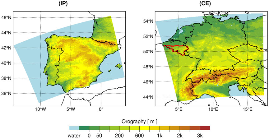
FIGURE 1. Orographic maps of the two considered domains for the climate simulations with COSMO-CLM: the Iberian Peninsula (IP) on the left and Central Europe (CE) on the right. The red border defines the Wallonia (Belgium) study case for the simulations with the dynamic vegetation models LPJ-GUESS and CARAIB. The analysis is restricted only to the land points of both domains.

The major added value of CPRCMs is a more realistic simulation of cloud dynamics and land-atmosphere interactions with better representation of heavy precipitations, especially in summer at mid-latitude where convective phenomena play a major role (Prein et al., 2015; Coppola et al., 2020; Pichelli et al., 2021). CPRCMs are therefore best suited for investigations about extreme precipitation events. Due to their fine resolutions, CPRCMs better represent the climate over complex terrains with strong spatial heterogeneities such as mountainous regions or coastlines, and might then become the tool to provide high-resolution input data for impact studies. Yet, these models have biases compared to observations (Ban et al., 2021). These errors can arise due to a variety of factors, such as incomplete knowledge of the physics of the climate system or errors in the representation of key processes. This complicates the direct use of CPRCMs data by impact modelers who require realistic unbiased climate data. Bias correction is a statistical technique that is used, and often considered a necessary step (Christensen et al., 2008), to adjust for the model output to better match observed data and improve the accuracy of climate projections.

Among the several bias correction methods in use (e.g., linear scaling, variance scaling, local intensity scaling, weather generators, quantile mapping, delta-change approach) (Maraun, 2016; Maraun and Widmann, 2018), we choose here a quantile-mapping approach (ISIMIP3) (Lange, 2019) which has the advantage of correcting the whole statistic of climate variables for each quantile and allows for a more robust bias correction of extreme quantiles (Lange, 2021a; Lange, 2021b).

Bias correction introduces, nevertheless, additional sources of uncertainty due to intrinsic assumptions such as the independence among climate variables, the type of transfer function chosen for each variable, or the bias stationarity across different climate conditions (Chen et al., 2011; Haerter et al., 2011; Ho et al., 2012; Van de Velde et al., 2022). These assumptions influence trends and consequently the climate change signal (Buser et al., 2009; Ehret et al., 2012), especially for absolute threshold-based climate indices (Dosio, 2016). At the local scale bias correction can even introduce corrections which can be larger than the signal itself (Hagemann et al., 2011; Maurer and Pierce, 2014).

For the latter reasons, this work aims to better understand the uncertainty of bias correction of high-resolution climate simulations. We, namely, investigate the impact of bias correction on climate change signals (CCSs) simulated by CPRCM by comparing raw and bias-corrected changes in climate variables such as seasonal precipitation, temperature, and climate extremes. It is also pivotal to understand how the uncertainty of bias correction propagates in impact models which make use of climate simulations. It is known, per example, that simulated precipitation is largely overestimated with respect to observations, a fact that can produce unrealistic results in climate change impact studies (Hagemann et al., 2013; Papadimitriou et al., 2016). This work adds to this discussion by analyzing the impact of bias correction on the CCS of vegetation variables simulated by two dynamic vegetation models, namely, LPJ-GUESS and CARAIB. Understand the impact of bias correction on projected changes of climate and vegetation variables is ultimately important for an open communication of risk assessment with stakeholders and policymakers.

The objectives of this manuscript are, namely, the following.

(1) What is the impact of bias correction on the CCS of seasonal temperature and precipitation?

(2) What is the impact of bias correction on the CCS of annual climate extreme indices?

(3) What is the impact of bias correction on the CCS of annual dynamic vegetation variables?

The structure of this manuscript is as follows: Section 2 presents the methodology, namely, the models used for climate and dynamic vegetation simulations, the statistical bias correction method, the analyzed climate and dynamic vegetation variables, and the statistical analysis to test the significance of climate changes. The methodology is summarized in the flow chart shown in Figure 2. Section 3 presents the results answering the three main questions of this manuscript. Section 3.1, Section 3.2, and Section 3.3 address, respectively, the first, second, and third objective of the manuscript. In Section 4 the results are discussed in the framework of impact model implications and the main conclusions and outlook are presented in Section 5.

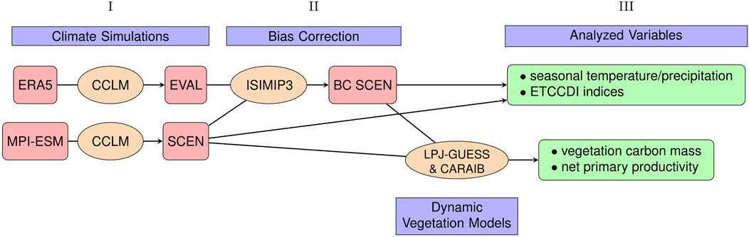
FIGURE 2. Flow chart summarizing the methodology. In the first step EVAL and SCEN climate simulations are performed by dynamically downscaling CCLM from the ERA5 reanalysis and the MPI-ESM GCM model, respectively. In the second step the ISIMIP3 method was used to bias correct SCEN based on EVAL. In the third step the climate change signal for climate and vegetation variables was computed from both bias-corrected and non-bias-corrected SCEN simulations. The vegetation metrics are the output variables from LPJ-GUESS and CARAIB forced by both bias-corrected and uncorrected climate simulations.

2 Materials and methods

The two study areas of our analysis are shown in Figure 1 and cover the Central Europe (CE) domain (42.82°N—55.28°N; 1.57°E—17.88°E) and the Iberian Peninsula (IP) (34.34°N—46.80°N; 14.5°W—4.01°E). The IP domain includes Spain, Portugal and part of southwestern France. The CE domain includes Belgium, the Netherlands, Luxembourg, Germany, Switzerland, Austria, northern Italy, eastern France, Slovenia, northern Croatia, Czechia, and western Poland.

The climate in these two regions is heterogeneous. The southern part of CE is influenced by the Mediterranean climate with mild and wet winters, and hot summers according to the Köppen-Geiger climate classification (Beck et al., 2018). The central and northern part of CE is characterized by the interaction between maritime and continental air masses such that the climate ranges from temperate in the west to cold in the east. Summers are warm with lower temperatures than in southern CE. The IP domain has a complex orography with several mountainous regions and due to its location in a transition zone between extratropics and subtropics, it is influenced by both Atlantic and Mediterranean climates. Northern IP has a temperate climate similar to the western part of CE with warm summers and without a dry season. The western and southern parts of IP have a Mediterranean temperate climate with dry and warm-to-hot summers. Central IP is instead more arid and dominated by xeric Mediterranean shrub vegetation.

2.1 Models simulations

2.1.1 Climate model simulations

Table 1 lists the climate model simulations conduced in this study over CE and IP. We have, namely, performed convection-permitting climate simulations, at a daily temporal resolution, by mean of the limited-area COSMO-CLM (herein abbreviated as CCLM) v5.16 model (Rockel et al., 2008; Baldauf et al., 2011).

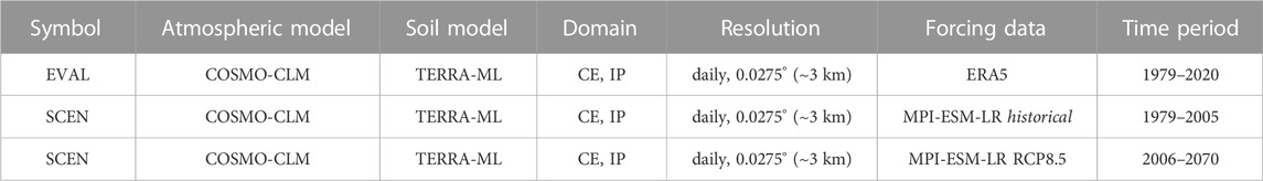
TABLE 1. List of climate model simulations conducted in this study. The year 1979 is considered as spin-up.

The evaluation simulations (EVAL) were conducted for the period 1979–2020 and driven by the ERA5 data which are global reanalysis data provided by the European Center for Medium-range Weather Forecast (ECMWF). ERA5 data have a time resolution of 1 h and an horizontal resolution of 0.25° (∼30 km) (Hersbach et al., 2018).

The scenario simulations (SCEN) were forced by the output data of the Max-Planck-Institute Earth System Model (MPI-ESM) model in the low resolution (LR) configuration, and cover a transient climatological period from 1979 to 2070. These GCM forcing data have a grid spacing of 200 km (150 km) in the atmosphere (ocean) and were provided within the framework of the Coupled Model Intercomparison Project phase 5 (CMIP5) (Giorgetta et al., 2013; Mauritsen et al., 2019). The historical experiment of CMIP5 provides global climate data until 2005, while the data from 2006 to 2070 have been obtained from the RCP8.5 experiment of CMIP5, which provides future climate projections under the RCP8.5 scenario (Giorgetta et al., 2012a; Giorgetta et al., 2012b). This scenario corresponds to a high radiative forcing (and concentration) pathway reaching more than 8.5 W/m² at the end of the 21st century (Meinshausen et al., 2011; Riahi et al., 2011; Vuuren et al., 2011).

Both ERA5 reanalysis data and GCM data from MPI-ESM have been directly downscaled with CCLM to a convection-permitting horizontal resolution of approximately 3 km leading to the EVAL and SCEN simulations, respectively. This first step is summarized on the left of the flow chart in Figure 2. For analysis, the year 1979 was discarded as spin-up year. CCLM is based on the fully compressible, non-hydrostatic thermodynamic equations in a moist atmosphere (Steppeler et al., 2003). These equations are numerically integrated on a Arakawa-C staggered grid (Arakawa and Vivian, 1977) in rotated coordinates with a Runge-Kutta RK3 time-splitting scheme (Wicker and Skamarock, 2002). The model uses a vertical terrain-following height coordinate (Doms and Baldauf, 2021). The precipitation is parameterized by a one-moment microphysics scheme which includes five categories of hydrometeors, i.e., cloud, rain, snow, ice and graupel (Doms et al., 2021), and soil processes are resolved by the multi-layer soil model TERRA-LM (Schulz and Vogel, 2020; Schrodin and Heise, 2001). Shallow convection is parameterized using a modified Tiedtke parameterization (Tiedke, 1989). The radiative transfer scheme is based on Ritter and Geleyn, 1992, and a turbulent kinetic energy-based surface transfer and planetary boundary layer parameterization have been used (Raschendorfer, 2001). The land-use classes are described by ECOCLIMAP (Masson et al., 2003; Champeaux et al., 2006) and the soil type and depth by HWSD TERRA (Smiatek et al., 2008).

2.1.2 Dynamic vegetation model simulations

Simulations with the dynamic vegetation model LPJ-GUESS (v.4.1) (Smith, 2001; Smith et al., 2014) and CARAIB (Warnant et al., 1994; Dury et al., 2011; Dury et al., 2018) were forced by the climate SCEN simulations (uncorrected and bias corrected) over the representative site of Wallonia in Belgium, see Figure 1.

Vegetation in LPJ-GUESS was simulated as potential natural vegetation with species-specific parameterization including the most common European tree species as well as typical shrub Plant Functional Types (PFTs), with a standard setup (Hickler et al., 2012). Nitrogen deposition input data were taken from (Tian et al., 2018).

The CARAIB model was set up to be as close as possible to the parameters of LPJ-GUESS. Vegetation in CARAIB is simulated as potential natural vegetation with the most common tree species in Wallonia. A 100-year spin-up is considered to reach equilibrium in the carbon pools and the climate data prior to 1980 were taken from the Global Soil Wetness Project Phase 3 (GSWP3) (Dirmeyer et al., 2006).

In both models the atmospheric CO₂ concentration data for (1900–2070) were taken from Meinshausen et al., 2011, and soil data were derived by aggregating the harmonized world soil database (Fischer et al., 2008). Since the simulated productivity of vegetation models is highly affected by solar radiation (Li et al., 2015), we used the raw solar radiation data in both simulations to investigate the influence of bias correction of temperature and precipitation on the output variables of LPJ-GUESS and CARAIB.

2.2 Statistical bias correction

Usual bias correction methods imply a statistical adjustment of climate simulation data in order to reduce deviations from observations. This adjustment is normally performed over a training historical period, typically of 30 years or longer, where observational data are available. For this study we have decided to apply a novel approach by using observation-based simulations instead of observational data as convection-permitting simulations are in the range of observational errors (Ban et al., 2021). We have, namely, bias corrected the scenario simulations on daily scale based on the evaluation simulations as schematically represented in the second step of the flow chart in Figure 2. Zhang and Tölle, 2021, have evaluated EVAL with respect to the HYRAS observational dataset over Germany (Razafimaharo et al., 2020), and they concluded that both spatial patterns and variability of daily precipitation and mean temperature are well represented by the evaluation simulations.

This approach has two advantages: first, both EVAL and SCEN have the same horizontal resolution such that they can be compared grid-cell-by-grid-cell without introducing uncertainties associated to statistical downscaling to the same grid spacing; second, the comparison is physically consistent since both simulations integrate deep-convection phenomena and share the same model configuration of CCLM.

The chosen statistical bias correction algorithm is the one provided within the Inter-Sectoral Impact Model Intercomparison Project phase 3 (ISIMIP3) (v2.5) (Lange, 2019; Lange, 2021b). The method is based on both parametric and non-parametric quantile mapping approach (Piani et al., 2010), which (i) adjusts biases in all percentiles of a distribution and (ii) approximately preserves trends in these percentiles. The method is independently applied to each variable (i.e., univariate bias correction), grid cell and calendar month. In particular, daily precipitation PR and mean temperature T are directly bias-corrected, whereas daily minimum TN and maximum TX temperature are indirectly corrected through daily temperature range T_rng = TX − TN and skewness T_sk = (T − TN)/T_rng. This procedure guaranties that relative errors for TN and TX have the same order of magnitude as for T (Piani et al., 2010).

In this section we refer to $x_{\text{hist}}^{\text{obs}}$ and $x_{\text{hist}}^{\text{sim}}$ as, respectively, the EVAL and SCEN in (1980–2020) for one climate variable, grid point and specific calendar month. For the same variable, grid point and month, $x_{\text{fut}}^{\text{sim}}$ and $y_{\text{fut}}^{\text{sim}}$ refer, respectively, to SCEN in (2021–2070) and corresponding bias-adjusted simulations. The ISIMIP3 method does not require that the future application period must be of the same length as the historical training period since the algorithm, as described below, is based on transfer functions. After training over the historical period, the bias correction was applied to the future period. $F_{\text{p}}^{\text{obs/sim}}(x)$ and ${\widehat{F}}_{\text{p}}^{\text{obs/sim}}(x)$ are the non-parametric (i.e., empirical) and parametric (i.e., fitted) cumulative distribution functions in the period “p”, respectively. The inverse function of F(x) $(\widehat{F}(x))$ is the quantile function Q(p) $(\widehat{Q}(p))$ such that, if p = F(x) is the cumulative probability for the value x then x = Q(p).

First, pseudo future observations are generated, $x_{\text{fut}}^{\text{obs}}$, by transferring the simulated CCS between $x_{\text{hist}}^{\text{sim}}$ and $x_{\text{fut}}^{\text{sim}}$ to $x_{\text{hist}}^{\text{obs}}$. This is achieved by using a non-parametric transfer function for every distribution quantiles rendering, therefore, the bias correction method trend-preserving in all quantiles.¹ Different trend preservation is applied to different climate variable as specified in Supplementary Table S1 in the Supplementary Material: it can be an additive trend preservation as for T, a multiplicative trend preservation or a combination of both as for PR and T_rng. For bounded variables like T_sk the trends are transferred respecting the bounds.

Pseudo future observations obeying additive trend preservation are generated via the following transformation

The transformation for multiplicative trend preservation reads

where

such that the relative simulated CCS, $Q_{\text{fut}}^{\text{sim}}/Q_{\text{hist}}^{\text{sim}}$, is transferred to $x_{\text{hist}}^{\text{obs}}$ with Δ_mul(p) bounded between 0.01 and 100. Eq. 2 can produce very large unrealistic values of x′ in case of very large negative simulation biases, namely, when $x_{\text{hist}}^{\text{obs}}\gg x_{\text{hist}}^{\text{sim}}$. To avoid such circumstances, pseudo future observations for PR and T_rng are obtained through a combination of Eqs 1, 2 according to

where

The function γ(p) smoothly interpolates between a multiplicative trend preservation in case of positive simulation biases and additive trend preservation for large negative biases.

For bounded variables such as T_sk, the trend transfer function reads

which preserves the a and b bounds.

The second step consists of a parametric quantile mapping to bias adjust future simulations $x_{\text{fut}}^{\text{sim}}$ to pseudo future observations $x_{\text{fut}}^{\text{obs}}$, and historical simulations $x_{\text{hist}}^{\text{sim}}$ to observations $x_{\text{hist}}^{\text{obs}}$.² The distributions used for this parametric quantile mapping are the Gaußian distribution for T, the gamma distribution for PR, and the Weibull distribution for T_rng. The variables with both upper and lower bounds, such as T_sk, are instead bias adjusted by using a non-parametric (i.e., empirical) quantile mapping.³

For the variable T, the bias correction at each quantile is obtained by applying a transfer function f(x) to, e.g., $x_{\text{fut}}^{\text{sim}}$ such that the fitted cumulative distribution function for $x_{\text{fut}}^{\text{sim}}$ equals the one for $x_{\text{fut}}^{\text{obs}}$ as

In case of an exact match between fitted and empirical cumulative distribution functions, the bias-corrected values $y_{\text{fut}}^{\text{sim}}$ would be equal to the pseudo future observations $x_{\text{fut}}^{\text{obs}}$. For the other considered variables, the quantile mapping is more involved since, in addition to biases in every quantiles, it also adjusts biases in the likelihood of individual events, similar to the scaled distribution mapping method introduced in (Switanek et al., 2017). In this case the bias-corrected future simulations are obtained through the transfer function defined via Eqs 10–14 in (Lange, 2019), which we do not report here for simplicity. For further technicalities of the ISIMIP3 method such as the conditional detrend for T, the randomization of values beyond thresholds, and the use of running windows we refer the reader to (Lange, 2019; Lange, 2021a).

2.3 Analyzed model output variables

The analyzed climate and vegetation variables are summarized in the third step of the flow chart in Figure 2.

2.3.1 Analyzed climate variables

2.3.1.1 Seasonal temperature and precipitation

Temperature and precipitation have been analyzed in their seasonal mean values and seasonal CCSs for both non-bias-corrected (nBC) and bias-corrected (BC) scenario simulations. Hereafter we will refer to the differences between BC and nBC results as statistical biases or simply biases. Let T_ij, TN_ij, TX_ij be the daily mean, minimum, maximum temperature on day i in a year j, respectively, and PR_ij the daily total precipitation amount. The seasonal mean value of, e.g., a temperature metric X = (T, TN, TX) in a period “p” is

where $\bar{X}$ is the spatial mean over the land points of CE or IP and the brackets ⟨⋯ ⟩ correspond to the temporal mean value. The following three 30-year climatological periods are assumed

where the base period includes years belonging to the historical and part of the RCP8.5 simulations of SCEN. This choice is justified by the fact that the training historical period—identified by the label “hist” in Section 2.2—used in the statistical bias correction method is 1980–2020. This training period serves therefore as reference period.

The seasonal CCS for temperature is computed as difference between the mean over a future period and the mean over the base period

For precipitation, we consider both relative as well as absolute seasonal differences with respect to the base period.

Where the factor 1/30 averages over the duration (in years) of base and future period.

2.3.1.2 Climate extreme indices

We additionally analyzed extreme events by computing the ETCCDI indices—introduced by the Expert Team on Climate Change Detection and Indices (Peterson et al., 1998; Karl et al., 1999)—which describe moderate to extreme aspects in daily temperature and precipitation statistics. These indices have been extensively used to study changes of extreme weather in observational data (Frich et al., 2002; Kiktev et al., 2003; Alexander et al., 2006; Min et al., 2011; Morak et al., 2011), model simulations of historical climate (Sillmann et al., 2013a) and for future climate projections as well (Sillmann and Roeckner, 2007; Tebaldi et al., 2007; Sillmann et al., 2013b; Rajczak and Schär, 2017; Putra et al., 2020; Wei et al., 2022).

Table 2 and Supplementary Figure S2 show the list of analyzed extreme indices with the corresponding definitions. Precipitation-dependent indices are computed from PR_ij whereas temperature-dependent indices are computed from T_ij, TN_ij, or TX_ij. Some of these indices, such as warm/cold days and nights, are based on percentile thresholds rather than absolute thresholds. The advantage of percentile threshold-based indices is that they represent, at each location, the same part of the probability distribution function and are therefore more representative over larger regions with complex topography and/or different climatological conditions (Radinović and Ćurić, 2011).

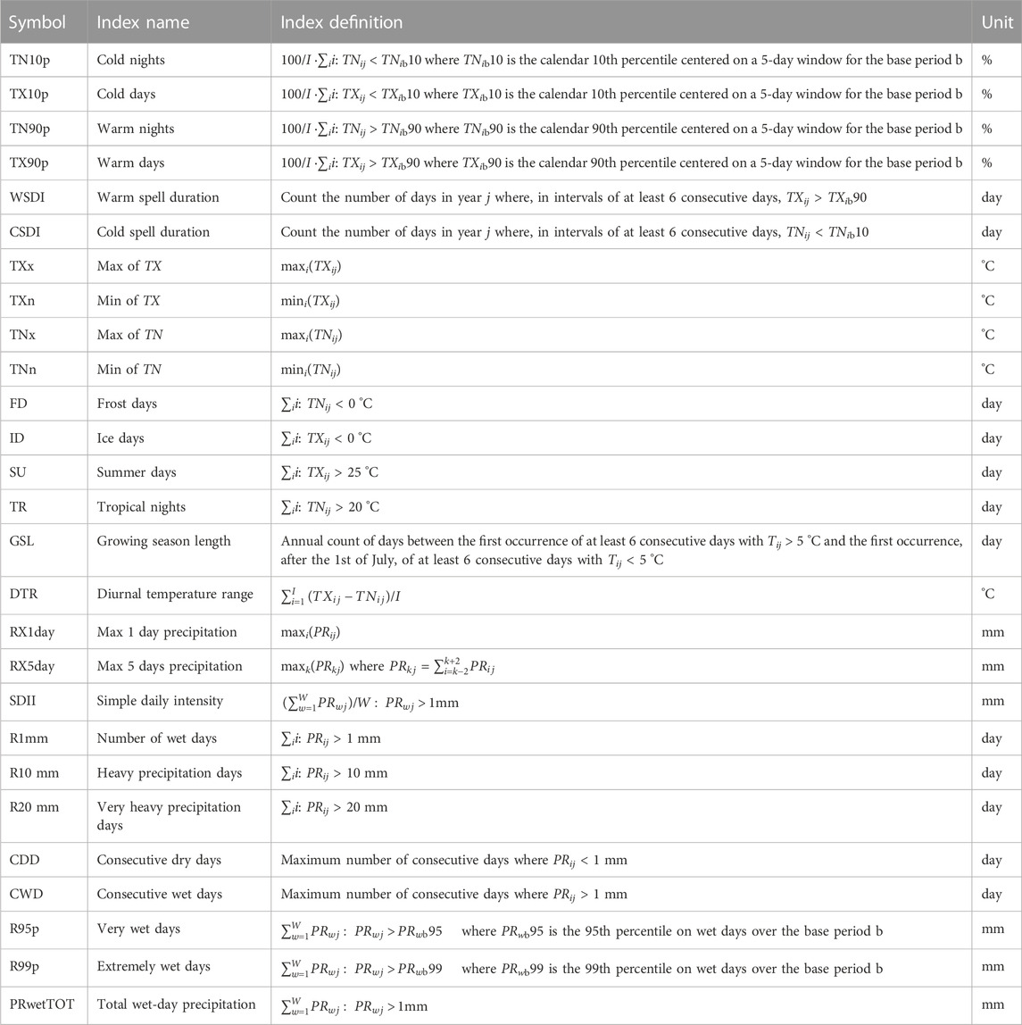
TABLE 2. List of analyzed extreme indices as recommended by the ETCCDI. TN_ij, TX_ij, and T_ij represent, respectively, the daily minimum, maximum, and mean temperatures on day i in the year j. I and W are the total number of days and wet days in the year j, respectively. The base period b has been chosen as the 30-year reference period (1981–2010).

We computed the whole set of indices for each year from 1980 to 2070 at each grid point of the two study domains. Given the annual time series ${\mathfrak{I}}_j$ for the index $\mathfrak{I}$ we analyzed the inter-annual variability of ${\bar{\mathfrak{I}}}_j$ and the spatial distribution of the climate change signals.

2.3.2 Analyzed vegetation variables

We additionally investigated the influence of bias correction on the CCS of two dynamic vegetation variables, i.e., carbon mass (cmass) and net primary productivity (NPP). With CARAIB, we investigated also the annual water stress mortality (Mw) coefficient which expresses the percentage of total biomass subject to water stress mortality. As a representative case we considered the site of Wallonia in Belgium, see Figure 1.

2.4 Test of significance of climate change signals

We use the statistical non-parametric two-tailed Wilcoxon-Mann-Whitney test to determine if there is a statistically significant change in climate variables (i.e., temperature, precipitation, extreme indices). This test is also known as the Mann-Whitney U test (Storch and Zwiers, 1999). It assess the significance of differences between two data sets representing the base and a future time periods. The test is based on the null hypothesis that there is no difference between the two groups being compared. It does not assume any particular distribution of the data, making it suitable for non-normal or skewed data often encountered in climate science. The test assigns ranks to the combined data from both groups and calculates the sum of the ranks for each group. The test statistic, U, represents the rank-sum of one group relative to the other. If the p-value is below a predetermined significance level (in this manuscript we use 0.05), the null hypothesis is rejected, indicating that there is a significant difference between the two groups in terms of the climate variable being studied.

3 Results

When presenting the spatial distribution of the CCSs for temperature, precipitation, and climate extreme indices we consider only those grid-points characterized by significant changes. The areas associated to non-significant changes are colored in gray whereas the full spatial distributions are shown in the Supplementary Material. For all tables showing the spatial mean CCSs of climate and vegetation variables, we report the corresponding p-value. Non-significant mean changes are highlighted in gray.

3.1 Impact of bias correction on climatic seasonal temperature and precipitation

3.1.1 Seasonal temperature

3.1.1.1 Mean seasonal values

The seasonal cycle of daily mean temperature over CE (IP) for the base period (1981–2010) is shown in the upper (lower) row of Figure 3, where a direct comparison between evaluation simulations and scenario simulations is provided. The left panels show the monthly mean values whereas the middle and right panels show the time Probability Distribution Functions (t-PDFs) of daily mean temperatures for winter (DJF) and summer (JJA), respectively. The differences between raw and bias-corrected model data with “observations” on spatial distribution in the historical period are provided in the Supplementary Material, see Supplementary Figures S3–S5.

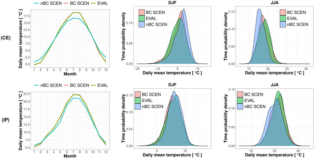
FIGURE 3. Season cycle of daily mean temperature T for Central Europe (upper row) and the Iberian Peninsula (lower row) over the base period (1981–2010). The left panels show the monthly mean values for bias-corrected (BC) and non-bias-corrected (nBC) scenario simulations (SCEN) as well as for evaluation simulations (EVAL). The middle and right panels represent the time probability distribution functions in winter (DJF) and summer (JJA), respectively.

The monthly mean temperatures obtained from the SCEN simulations become closer in magnitude to the values computed from EVAL after bias correction, with maximum differences of ±0.3 °C for CE and ±0.2 °C for IP, see left panels in Figure 3. The t-PDFs in summer for the BC simulations are in fact shifted towards higher temperatures with a good overlap with the t-PDFs for EVAL. This shift is particularly pronounced in the upper tail of the probability distribution for CE. Opposite situation occurs in winter, which becomes cooler after bias correction with a shift towards lower temperatures of the t-PDFs. This shift is less pronounced in IP than CE. Similar conclusions can also be drawn for TN and TX as shown, respectively, in Supplementary Figure S1 and Supplementary Figure S2 in the Supplementary Material.

Supplementary Table S3 reports the seasonal mean values for T, TN and TX in the three climatological periods over CE and IP for both raw and bias-corrected scenario simulations. The winter mean temperature values in CE are reduced after bias correction by about range − 1.3–1.1 °C in all periods while the reduction of winter mean temperatures in IP is less pronounced ranging within −0.9 ÷ 0 °C. Only the winter mean value of TX in IP is not affected by bias correction, which is in agreement with the nearly unchanged t-PDF of TX in DJF shown in Supplementary Figure S2. In summer, the mean temperature values are higher in the BC simulations compared to the raw climate simulations. The mean warm bias in summer is within 0.8 ÷ 2.7 °C in CE and 0.4 ÷ 1.9 °C in IP with the warmest bias for TX. Bias correction introduces a warm bias also in spring/autumn in IP for all temperature metrics. In CE bias correction increases TX and decrease TN in spring/autumn by about half a degree Celsius with nearly no impact for T.

3.1.1.2 Mean seasonal CCSs

Despite the presence of biases in the absolute mean seasonal temperature values, the impact of bias correction on the mean seasonal CCSs is negligible as the difference between raw and bias corrected mean changes does not exceed 0.1 °C in all seasons, temperature metrics, and both domains. This is shown in Table 3 where the mean and standard deviation for the seasonal CCSs of temperature metrics in both domains is reported.

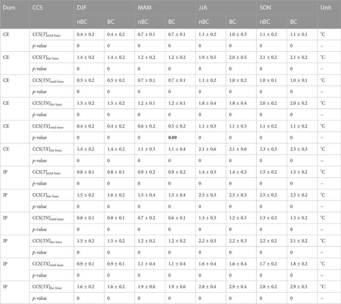
TABLE 3. Mean ± sd (standard deviation) for the spatial distribution of changes CCS_mid-base and CCS_far-base for the metrics T, TN, and TX for winter (DJF), spring (MAM), summer (JJA), and autumn (SON) over both domains. Results are rounded to the precision of 0.1 °C and computed for both nBC and BC scenario simulations. The p-value of the two-tails Wilcoxon-Mann-Whitney test shows the significance of mean changes: non-significant mean CCSs (p-value >0.05) are highlighted in bold.

Table 3 shows that under RCP8.5 scenario, seasonal temperatures are projected to increase with a stronger warming in the far future period than mid-future. Over the CE domain, summer and autumn will experience the strongest warming across all seasons with a far future increase of all temperature metrics between 1.8 ÷ 2.3 °C, while the far future warming in winter and spring ranges within 1.1 ÷ 1.5 °C. The increase of temperatures over the Iberian Peninsula is stronger than in CE with also summer/autumn seasons more affected than winter/spring. The far future increase of temperatures over IP is about 2.2 ÷ 2.8 °C in summer/autumn and 1.2 ÷ 1.9 °C in winter/spring.

3.1.1.3 Spatial variability of seasonal CCSs

Figure 4 shows the spatial patters of the seasonal CCSs for TX between far future and base period. The CCS is statistical significant in all grid-points and seasons.

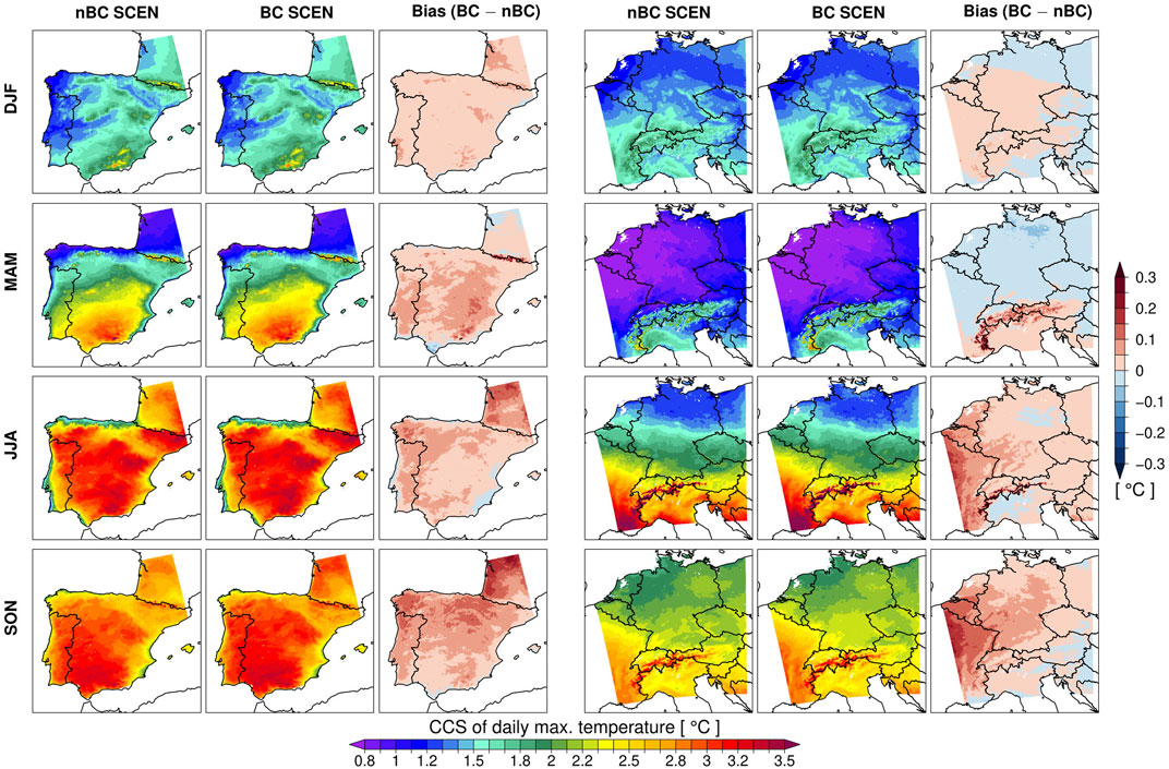
FIGURE 4. Spatial distributions of seasonal climate change signals (CCSs) between (2041–2070) and (1981–2010) for daily maximum temperature TX over the Iberian Peninsula (left panels) and Central Europe (right panels). The CCSs are computed for the bias-corrected (BC) and non-bias-corrected (nBC) scenario simulations (SCEN). Biases are measured as differences between BC and nBC results. The CCS at every grid points is significant (p-value ≤0.05).

The warming of TX in CE is characterized by a general south-north gradient across all seasons with stronger warming in the southern regions. This gradient is particular emphasized in summer where the warming ranges from 1.2 °C in northern CE to 3.6 °C in southeastern France with peak values of 4.6 °C (out of the color scale) over the Alps. The Alps feature the strongest warming within the CE domain also in spring and autumn with an increase of TX by more than 2 °C and 3 °C, respectively.

The CCS for TX in winter over IP shows an orographic dependence with the strongest warming (within 2.2 ÷ 3 °C) over the Pyrenees and Baetic System in southern Spain. The warming of TX in spring has a south-north gradient ranging from 1 °C in southwestern France and Spanish Atlantic coast to 3 °C in southern Spain. The increase of TX in summer and autumn in IP is generally lower along the coastal areas than in the hinterland. The highest CCS in JJA is of 3.4 °C in limited areas in central eastern Spain while the highest CCS in SON is of 3.2 °C in southern Spain.

The local biases on the seasonal far future CCSs are generally negligible ranging within ±0.2 °C in both domains. Bias correction slightly enhances the warming of TX in summer and autumn over CE, and in all seasons over IP. The highest biases have been found in spring over the Pyrenees and Maritime Alps, where the warming is enhanced by 0.3 °C and in summer over the western and central Alps, where bias-corrected CCS is higher by approximately 0.5 °C.

Supplementary Figure S3 and Supplementary Figure S4 in the Supplementary Material show the spatial patters of the far future seasonal CCSs for daily mean and minimum temperatures, respectively. All differences are statistical significant. The warming of TN is lower than TX over both domains, indicating that changes in the upper tail of temperature distribution are larger than changes in the lower tail. Similarly to TX, the seasonal CCSs of T and TN are larger over high mountainous regions and the warming of T and TN in summer is characterized by a south-north gradient in CE. The impact of bias correction on the seasonal CCSs of T and TN is negligible ranging within ±0.15 °C across both domains.

3.1.2 Seasonal precipitation

3.1.2.1 Mean seasonal values

Figure 5 shows the seasonal cycle (left panels) as well as the time probability distribution function in winter and summer (middle and right panels, respectively) for daily precipitation sum over CE (upper row) and IP (lower row) for the base period (1981–2010). The differences between raw and bias-corrected model data with “observations” on spatial distribution in the historical period are provided in the Supplementary Material, see Supplementary Figure S6.

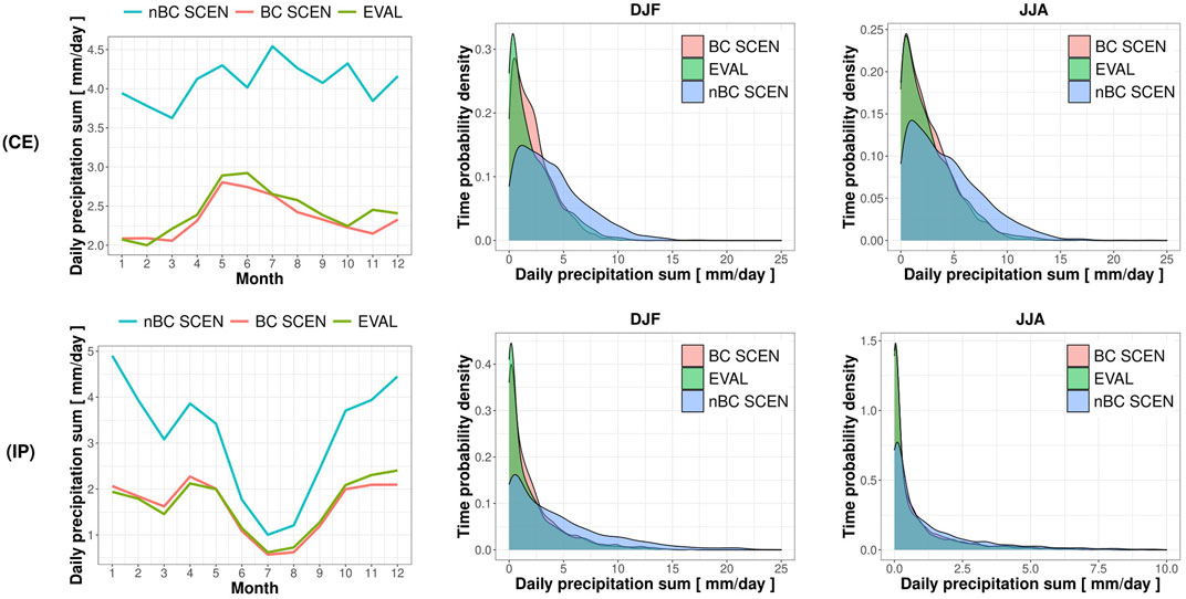
FIGURE 5. As in Figure 3 but for daily precipitation sum PR_ij.

The raw SCEN simulations overestimate monthly mean precipitation by a factor of 1.4÷2.5 with respect to EVAL, see the left panels in Figure 5. Bias correction not only reduces the absolute amount of rainfall but also adjusts the inter-monthly variability especially for CE with peak values in May-June, see upper left panel in Figure 5. After bias correction the monthly mean daily precipitation of SCEN are similar in magnitude to the values of EVAL; yet small differences within −12 ÷ + 4% for CE and −14 ÷ + 11% for IP are still present. Due to the reduction in magnitude of PR after bias correction, the t-PDFs are squeezed toward lower precipitation values with a consequent increase in the frequency of low-intensity precipitations, see middle and right panels of Figure 5. Bias correction thus increases the frequency of dry events in agreement with the EVAL simulations.

The reduction in magnitude of precipitation due to bias correction also holds for the future periods as reported in Supplementary Table S4, which shows the seasonal daily mean values of PR for both domains and both raw and corrected scenario simulations. In Central Europe, the simulated daily precipitation amounts are reduced by about −45 ÷ − 37% and in IP by approximately −55 ÷ − 40% after bias correction. The strongest impact of bias correction on the magnitude of precipitation is in winter for both domains.

3.1.2.2 Mean seasonal CCSs

Table 4 shows the spatial distribution properties (mean and standard deviation) of the seasonal CCSs for PR computed over the land points where the mean daily precipitation in the base period is above 1 mm/day in order to exclude drizzle. The CCS is computed both as relative and absolute difference with respect to the base period according to Eqs 11, 12.

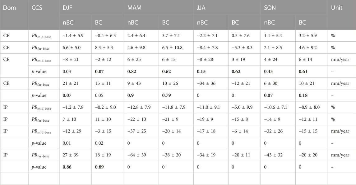
TABLE 4. As in Table 3 but for mean changes in seasonal precipitation sum. The CCSs are given both as relative differences and anomalies with respect to the base period according to Eqs 11, 12. The grid-points with mean precipitation lower than 1 mm/day (dry/wet threshold) in the base period are excluded from the calculation of mean and std values. These grid-points are stippled in Figure 6. Non-significant mean changes (p-value >0.05) are highlighted in bold.

In Central Europe, precipitation is projected to significantly increase by about 8% in winter in the far future in the BC simulations. Contrary to this, summer precipitation in CE is projected to significantly decrease by about −8% and −5% in the far future in the nBC and BC simulations, respectively.

Over the Iberian Peninsula, precipitation is projected to significantly decrease in spring, summer, and autumn in both nBC and BC simulations. The uncorrected simulations project, namely, a far future reduction of rainfalls over IP by about −64 mm/year (−22%) in spring, −34 mm/year (−19%) in summer, and −43 mm/year (−14%) in autumn.

The impact of bias correction on the relative mean seasonal changes in precipitation is small over both domains. In particular the projected decrease of summer precipitation over CE (IP) is reduced in absolute value by about 34)% after bias correction due to a small wet, i.e., positive, bias contribution.

3.1.2.3 Spatial variability of seasonal CCSs

Figure 6 shows the spatial patterns of significant seasonal changes in precipitation over both domains for the far future period. The gray areas are characterized by non-significant changes, whereas the stippled areas correspond to those grid points with a mean daily precipitation in the base period below the dry/wet threshold of 1 mm/day. Supplementary Figure S16 shows the far future seasonal CCSs of precipitation at all grid points.

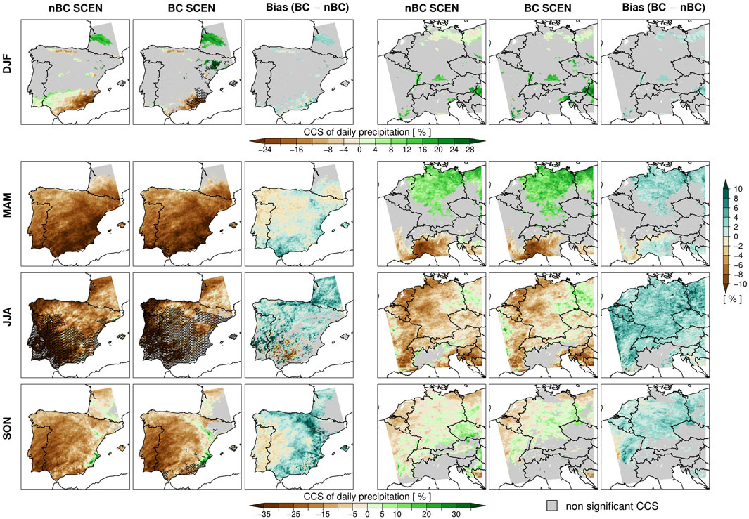
FIGURE 6. As in Figure 4 but for daily precipitation sum PR. The stippled area corresponds to the regions where the mean daily precipitation in the base period (1981–2010) is below 1 mm/day (dry/wet threshold). Grid-points with non-significant changes are colored in gray.

Northern and southern Spain are characterized by a significant reduction of winter precipitations with stronger decreases of −28% in southeastern Spain. A significant increase in winter precipitations of about 30% is simulated over few areas in eastern Austria and northeastern Spain.

Spring precipitations are projected to significantly decrease across the whole IP domain with strongest CCSs in eastern Spain of about −50 ÷ − 40% (out of the color scale). On contrary simulations over CE suggest a significant increase of precipitation in MAM in northern/central Germany and Poland (with highest values about 20 ÷ 30%) and a significant decrease in northern Italy (with lowest values of about −30%).

In summer, the precipitation is projected to significantly decrease over most of the CE domain and in northern IP. The dry regions in southern/central IP (stippled area in Figure 6) remain dry also in the far future due to further significant decreases in precipitation. The strongest significant decrease of summer precipitation lower than −30% is simulated in northwestern IP and southeastern CE. On contrary, a significant increase of summer precipitation up to 20% is projected in western Poland.

Autumn precipitation is projected to significantly decrease across most of the IP domain with the lowest values of about −40% in southwestern IP. Few areas in eastern Spain exhibit a significant increase up to 40% in autumn precipitation. The decrease of autumn precipitation in northern CE is also significant but less severe than IP and not lower than −20%. A small significant increase of autumn precipitation in CE is simulated in Germany, Poland, and Austria over mountainous regions.

Bias correction mostly introduces a wet (positive) contribution, which locally does not exceed 12%. Small dry biases, instead, are found in western IP during spring and autumn. The stippled area in IP obtained from BC simulations is larger compared to raw simulations in all seasons. This is because the reduction in magnitude of precipitation after bias correction turns many wet days into dry days.

3.2 Impact of bias correction on the CCS of climate extreme indices

3.2.1 Temperature-dependent ETCCDI indices

3.2.1.1 Inter-annual variability

Figure 7 shows the inter-annual variability for the annual maximum values of TX, frost days, growing season length, tropical nights, summer days, and warm days for both nBC and BC simulations. For each index the upper (lower) plot refers to CE (IP).

FIGURE 7. Inter-annual variability of the spatial mean value (over land points only) for some of the temperature-dependent ETCCDI indices given in Table 2. Except for the percentile index TX90p, differences with respect to the average over the (1981–2010) base period are displayed. To smooth the trends, a centered 11 years running mean filter is applied. The solid blue (red) line shows the results for the uncorrected (bias-corrected) scenario simulations.

The annual maximum values of TX (TXx) can increase by up to 4 °C by the end of the investigation period in both domains. Bias correction slightly projects higher future values of TXx in CE, yet not more than 0.5 °C.

Frost days (FD) decrease up to −25 (−12) days/year in CE (IP) by 2070. Bias-corrected simulations project up to 5 frost days per year less than raw simulations which can be explained by the warm bias of TN in winter, see Supplementary Figure S4.

The thermal growing season is projected to last longer in a warmer climate with an increase of its duration by up to 35 (20) days/year in CE (IP) at the end of the investigation period. Bias correction slightly reduces the future positive trend of GSL over CE, while it enhances the trend over IP. The annual mean differences between nBC and BC values do not exceed ±5 days/year.

The increases of tropical nights (TR) and summer days (SU) are more severe over IP than CE. Uncorrected SCEN simulations project an increase up to 7 (20) days/year for TR and 20 (35) days/year for SU in CE (IP). Bias correction further increases the projected future values of TR and SU by up 5 days/year, which can be explained by the warm bias in the summer daily temperatures, see Figure 4 and Supplementary Figure S3.

The positive trends in warm days (TX90p) indicate that the upper tail of the distribution function for TX is shifted toward warmer temperatures in the future. The exceedance rate of warm days is projected to increase from the nominal value of 10% in the base period to 25 (30)% by 2070 over CE (IP) with a negligible impact of bias correction.

Supplementary Figure S5 and Supplementary Figure S6 show the inter-annual variability for the remaining temperature indices. The annual extreme values of TN and TX show large inter-annual oscillations with respect to their mean positive trends, especially in CE. The increase of GSL leads to an earlier start of the growing season which is anticipated by about 20 (12) days in CE (IP). Bias correction slightly shifts GSS later (earlier) in time over CE (IP), which is consistent with the impact of bias correction on GSL. The inter-annual variability for warm spell duration (WSDI), number of warm spell (nWSDI), and warm nights (TN90p) is qualitatively similar to TX90p shown before. Cold nights and days (TN10p and TX10p, respectively) decrease from the nominal 10% in the base period to 2 ÷ 3% by the end of the investigation period. Both upper and lower tails of the distribution of TX and TN are thus projected to move towards warmer temperatures. The impact of bias correction on the inter-annual variability of cold/warm nights, cold/warm days and cold/warm spell duration is negligible.

Generally, the variability of temperature indices is not modified by bias correction. The bias correction has minimal impact on the mean climate change signal of percentile indices, as the difference between the raw and bias-corrected simulation data is small. Yet, quantile mapping modifies the magnitude of changes for those indices based on absolute thresholds.

3.2.1.2 Mean climate change signals

The spatial mean and standard deviation for the CCSs of all temperature indices are summarized in Supplementary Table S5 and Supplementary Table S6. The significance (p-value) of the mean changes are also reported.

Under RCP8.5 scenario, temperature indices such as warm days/nights, warm spell duration, summer days, tropical nights, and growing season length have significant positive future trends while indices such as cold days/nights, ice and frost days are projected to significantly decrease over both domains. The far future CCSs are also larger, in absolute value, than the mid-future changes.

The warming of temperatures belonging to the upper tail of the time distribution is stronger than the warming of the lower tail. The mean increase of warm days/nights of about 12 ÷ 17% is in fact larger than the mean decrease of cold days/nights of −6%. The warming of extreme maximum temperatures (TXx and TNx) is also larger than the corresponding warming of extreme minimum temperatures (TXn and TNn).

The impact of bias correction on the spatial mean changes of temperature indices is marginal. In fact, the mean biases do not exceed 0.8%, 0.2 °C, and 4 days/year for percentile indices, indices measuring temperatures, and duration indices, respectively.

3.2.1.3 Spatial variability of climate change signals

Figure 8 shows the spatial patterns of significant mid- and far future changes for the annual maximum of TX (TXx), growing season length (GSL), summer days (SU), and tropical nights (TR). For completeness, Supplementary Figure S17–Supplementary Figure S19 show changes at all grid-points.

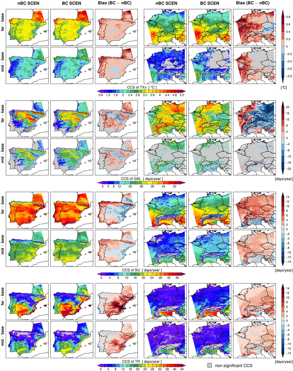
FIGURE 8. Spatial distribution of significant mid- and far future changes for annual maximum of TX (TXx), growing season length (GSL), summer days (SU), and tropical nights (TR). Results are shown for bias-corrected (BC) and uncorrected (nBC) scenario simulations, while the impact of bias correction is shown as difference between BC and nBC results. Grid-points with non-significant changes are displayed in gray.

The far future warming of TXx is significant over both domains and reaches about 5 °C with the strongest signal simulated in northern Spain, southwestern and eastern France. Peaks of 5 ÷ 6 °C are simulated in limited area over the Swiss Alps. Statistical biases range mainly within ±0.4 °C with larger positive values of about 1 °C located in eastern France, Belgium, the Netherlands, and in southwestern France. Large biases of about 2 °C (outside the color scale) are found over small areas in the western and central Alps, where the far future increase of TXx can reach up to 8 °C in BC simulations.

Over the IP domain, changes in GSL larger than 8 days/year are significant in both future periods. In Central Europe, the mid-future changes of GSL are significant in northern and southern CE while the far future changes of GSL are significant over the whole domain. The significant increases in GSL reach up to 36 (44) days/year in the mid-future and 52 (60) days/year in the far future over CE (IP). The growing season is, namely, projected to be 1 month longer in the far future across most of the CE domain with large changes simulated in northeastern Germany, western Poland, the Alps, and small areas across Germany, Austria, eastern France, and southern Belgium. Mountainous regions in IP are characterized by a strong increase of GSL up to 44 days/year in the mid-future and 60 days/year in the far future. Statistical biases have a large spatial variability over both domains ranging within ±24 (±14) days/year over CE (IP) in the far future. Large warm biases are found over lower terrains in western/southern CE while negative biases are mainly in central and eastern CE. Consequently, the highest changes in GSL over CE are shifted towards the western regions. Over the IP domain, bias correction introduces a cooling effect (i.e., a decrease of CCS) over mountainous regions and a warming effect elsewhere.

The summer days index is projected to significantly increase in both domains except over the Alps. The largest increases are simulated in southeastern France, hillsides of the Italian Alps and Apennines, southeastern regions of CE, eastern and southern Spain where changes in SU reach up to 26 days/year in the mid-future and 40 days/year in the far future. Bias correction modifies the spatial distribution of the CCS for summer days due to the large variability of statistical biases ranging within ±14 days/year. Positive biases are found across the whole CE domain (except for the southern regions) and over the lower terrains in northern and western IP.

The significant mid-future changes of tropical nights in CE is less than 10 days/year across the whole domain except for the Po valley where increases of TR ranging within 14 ÷ 24 days/year are simulated. This positive trend over the Po valley is exacerbated in the far future when the CCS reaches up to 44 days/year at the Adriatic coast. Easter France and southeastern regions in CE experience an increase of TR between 14 ÷ 30 days/year in the far future. Tropical nights increase across the whole IP domain except for mountainous regions. The highest significant changes in IP are simulated over the Mediterranean coasts and Balearic Islands, where TR increases by up to 30 days/year in the mid-future and 46 days/year in the far future. The hillsides of Sierra Morena along the Guadalquivir River in southern Spain and the Ebro valley in northern Spain show also large increases of TR by up to 26 days/year in the mid-future and 38 days/year in the far future. Biases mitigate by up to −8 days/year the increase of TR over the Po valley and Mediterranean Spanish coasts. The largest positive biases are found in southeastern France, the hillside regions of the Italian Alps, and central/northeastern Spain where biases can reach up to 10 days/year in the mid-future and 16 days/year in the far future.

Supplementary Figure S7–Supplementary Figure S10 show the spatial patterns of significant changes for the remaining temperature indices. Changes in the percentile indices warm days/nights and warm spell duration are significant at all grid points. The CCSs for warm days (TX90p) have a south-north gradient over both domains with greater positive values in the southern regions, see Supplementary Figure S7. The exceedance rate of warm days is projected to increase the most over the Alps, Pyrenees, Baetic System, and Sierra Morena where the CCS is higher than 22% in the far future. Similar conclusions can be drawn warm nights (TN90p). Bias correction slightly mitigates the increase of warm days/nights across most of the CE domain and in northeastern IP. An additional positive contribution to the CCS of warm days/nights up to 4% due to bias correction is found in southern Spain and along the coastal areas of the Ligurian Sea. Changes in warm spell duration (WSDI) and number of warm spells (nWSDI) are qualitative similar to those for warm days. In particular, the strongest CCSs of WSDI are simulated over the Alps, Pyrenees, Baetic System and Sierra Morena where the far future increase of WSDI reaches about 50 days/year in the far future for nBC simulations and about 60 days/year after bias correction. The decreases in frost days (FD) lower than −8 days/year are significant in both domains. The changes of FD show a strong orographic dependence in the nBC simulations reaching up to −48 days/year in the far future over the Alps, Pyrenees, and Baetic System, see Supplementary Figure S9. These strong decreases are attenuated by bias correction, which introduces up to 12 frost days per year compared to nBC simulations. On contrary, bias correction reduces frost days on lower terrains by further decreasing FD up to −10 days/year in central Spain, Ebro valley, eastern France, and Belgium compared to nBC simulations.

The warm bias in southern IP found for temperature indices such as warm days/nights, warm spell duration, summer days and tropical nights can be associated to the dryer conditions, especially in summer, in the BC simulations, see Figure 6. More extended areas with water scarcity can in fact induce warmer daily and nocturnal conditions due to a reduction in evapotranspiration that can last longer in time.

3.2.2 Precipitation-dependent ETCCDI indices

3.2.2.1 Inter-annual variability

Figure 9 and Supplementary Figure S11 show the inter-annual variability for the precipitation indices. The changes in those indices measuring precipitation amounts and counting days or dry/wet periods are expressed as relative and absolute differences with respect to the base period average, respectively.

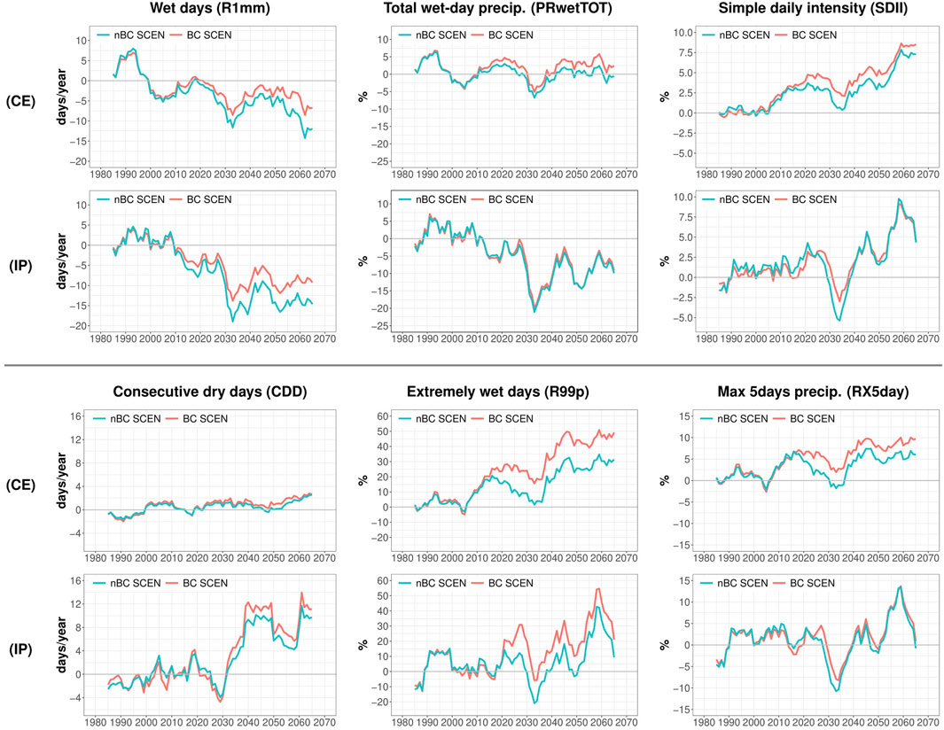
FIGURE 9. Inter-annual variability of the spatial mean value (over land points only) for some of the precipitation-dependent ETCCDI indices given in Table 2. R1mm and CDD are shown as anomalies with respect to the average over the (1981–2010) base period. PRwetTOT, SDII, R99p, and RX5day are shown as relative difference with respect to the base period average. To smooth the trends, a centered 11 years running mean filter is applied. The solid blue (red) line shows the results for the non-bias-corrected (bias-corrected) scenario simulations.

The number of wet days (R1mm) is projected to decrease over both domains up to −15 days/year by 2070 for nBC simulations, see Figure 9. Bias correction introduces more wet days in the future projections but not more than 6 days/year. The total annual precipitation on wet days (PRwetTOT) is projected to decrease in IP up to −10% by 2070 with peak of −20% in the mid-future while it oscillates within ±5% in CE.

The mean daily precipitation on wet days (SDII) is projected to increase over both domains. In particular, the positive trend of SDII in IP indicates that the decrease of wet days is stronger than the decrease of annual precipitation on wet days.

The decrease in wet days leads to increases of consecutive dry days (CDD) especially over the IP domain where CDD reaches up to +12 days/year by 2070 for nBC simulations. Bias correction further exacerbates the future projected values of CDD over the IP domain which is explained by the larger dry areas (especially in summer) in BC simulations as previously shown in Figure 6.

Extreme precipitation events are projected to increase over both domains as shown by the indices R99p, RX5day in Figure 9 and by the indices R95p, RX1day in Supplementary Figure S11. These positive trends are stronger in CE than IP but the inter-annual variability is larger in IP than CE. For example, the increase of R99p in the far future is about 40 ÷ 50% in CE while it oscillates between −4 ÷ + 40% in IP for nBC simulations. Bias correction further exacerbates the projected increases of extreme precipitations due to statistical biases which can reach up to 20% for R99p, 9% for R95p, 6% for RX1day, and 4% for RX5day.

Generally, bias correction does not modify the inter-annual variability of precipitation indices but modifies their magnitude amplifying projected relative changes. This is due to the reduction in magnitude of daily precipitation over the base period resulting in larger relative future changes and to the wet bias in the seasonal precipitation changes.

3.2.2.2 Mean climate change signals

Table 5, Supplementary Figure S6 and Supplementary Figure S7 summarize the mean values and standard deviations of the spatial distribution of the CCSs for precipitation indices. All grid points over land are considered and the significance of mean changes is also reported.

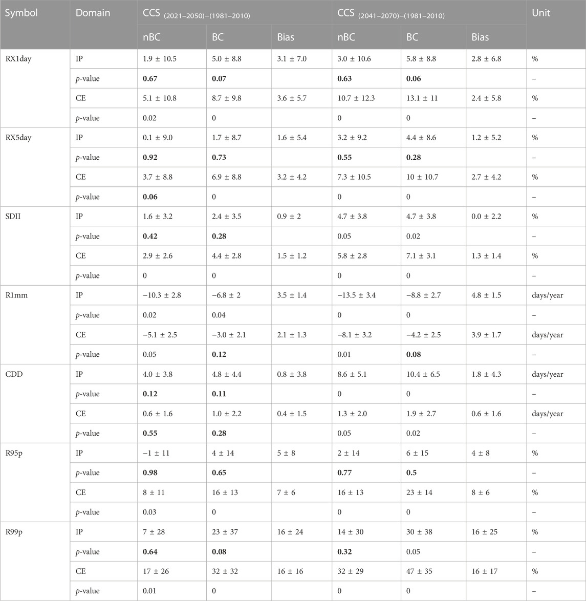
TABLE 5. Mean ± std (standard deviation) for the spatial distribution of mid- and far future changes of precipitation-dependent ETCCDI indices computed over the land points of Central Europe (CE) and the Iberian Peninsula (IP). The bias is computed as difference between bias-corrected (BC) and uncorrected (nBC) CCSs. The p-values of the two-tails Wilcoxon-Mann-Whitney test on the spatial mean CCSs are also reported. Non-significant mean changes (p-value >0.05) are highlighted in bold.

We can generally observed that, under the RCP8.5 scenario, precipitation events are generally projected to become less frequent but more intense, especially in CE, with an exacerbation of dry conditions in both domains. The number of wet days is projected in fact to significantly decrease while the annual precipitation above the 99th percentile of the base period is projected to significantly increase in the far future over both domains. Central Europe is also characterized by a significant increase of further indices associated to extreme events such as the maximum precipitation in one/5 days and the annual precipitation above the 95th percentile of the base period. Consecutive dry periods are expected to become longer in the far future due to a significant increase of CDD especially over the Iberian Peninsula.

Bias correction introduces a wetting condition on the CCSs for extreme precipitations especially over the CE domain. The spatial mean biases for R95p and R99p are, namely, 8 4)% and 16 (16)% in CE (IP), respectively. The mean impact of bias correction on the other precipitation indices is small and does not exceed 3% for percentile indices and 5 days/year for duration indices.

3.2.2.3 Spatial variability of climate change signals

Figure 10 shows the spatial distribution of significant changes in the number of wet days (R1mm), mean wet-day precipitation (SDII), consecutive dry days (CDD), and total annual precipitation on extremely wet days (R99p). Changes in precipitation amounts are expressed as relative differences with respect to the base period. For completeness, Supplementary Figure S22–Supplementary Figure S25 show changes at all grid-points. Differently from temperature indices, the CCS for precipitation indices is significant only over few regions. This is because precipitation indices have locally a large inter-annual variability such that a statistical analysis for seasonal time-series might be more informative. Some areas can in fact be characterized by significant changes in precipitation only for specific seasons. We leave this analysis for further studies.

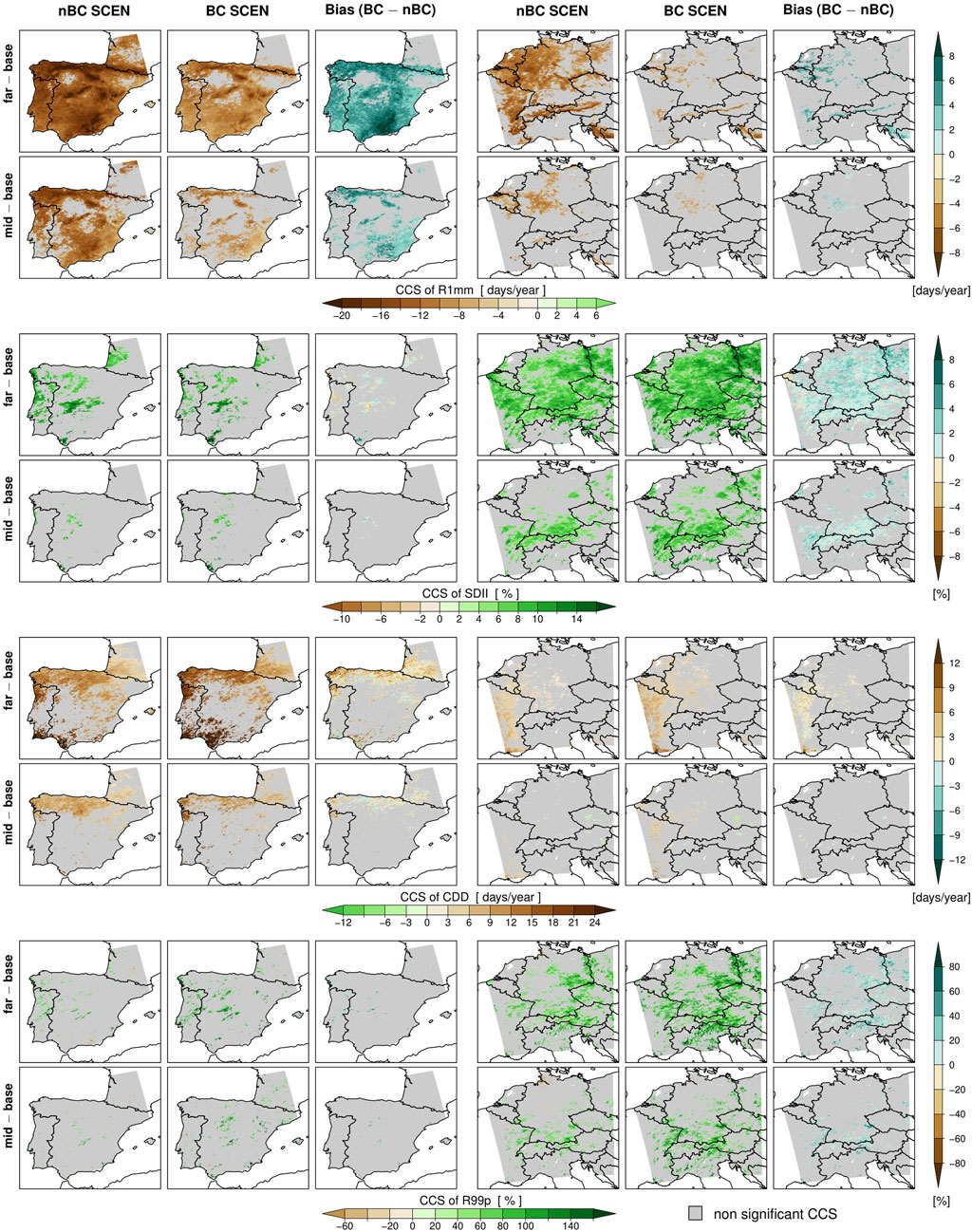
FIGURE 10. Same as in Figure 8 but for the number of wet days (R1mm), mean daily precipitation on wet days (SDII), consecutive dry days (CDD), and total annual precipitation on extremely wet days (R99p). Significant changes in precipitation amounts are shown as relative differences with respect to the base period. Grid-points with non-significant changes are displayed in gray.

The number of wet days is projected to significantly decrease over both domains especially over mountainous regions. The reduction is stronger in IP than CE and can reach up to −20 days/year for uncorrected simulations. In the bias-corrected simulations, the reduction of R1mm remains significant over mountainous regions even though the magnitude is reduced due to wet (positive) biases.

The mean daily precipitation on wet days is projected to increase in the far future by up to 14 (20)% in CE (IP) as for nBC simulations. This increase is significant over most of the CE domain, while in IP it is significant in central/southern Spain. In Central Europe SDII is further augmented by bias correction due to wet biases up to 10%.

The consecutive dry days index is projected to significantly increase in northern/southern IP and western CE with more severe changes in IP. Over these regions, bias correction exacerbates the duration of dry periods due to biases up to 14 days/year. Droughts are more sever in southern IP where BC simulations project a far future increase of CDD up to 40 days/years (out of the color scale). This might be due to the dryer condition in summer over IP, see Figure 6.

The total annual precipitation above the 99th percentile of the base period has a significant increase over mountainous regions in CE and central IP with a raw CCS up to 120% in northern Italy, Austria, southern/eastern Germany, and central IP. Bias correction intensifies these changes due to wet biases that can locally reach up to 100%. Similar conclusions are also valid for other extreme precipitation indices such as the total precipitation above the 95th percentile of the base period or the maximum precipitation amount in 1- or 5-day, which also display significant increases over mountainous regions in central IP and CE, see Supplementary Figure S13.

The spatial patterns of significant changes for the remaining precipitation indices are shown in Supplementary Figures S14-S16 and in Supplementary Figure S12 and Supplementary Figure S13.

3.3 Impact of bias correction on the CCS of dynamic vegetation model output variables

Table 6 shows the spatial mean and standard deviation of the bias-corrected and uncorrected CCSs for total carbon vegetation mass (cmass) and net primary productivity (NPP) over Wallonia (see Figure 1) as simulated by LPJ-GUESS and CARAIB. The significance of mean changes is also reported.

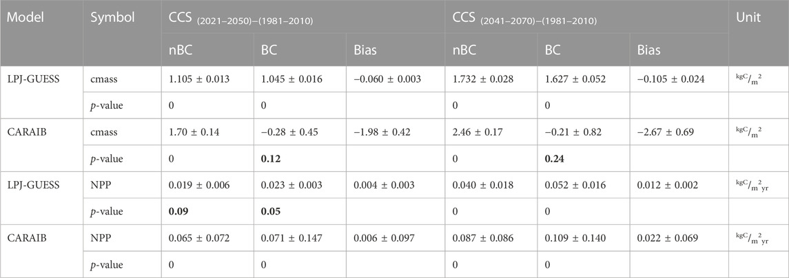
TABLE 6. Mean ± std (standard deviation) for the spatial distribution of the mid- and far future changes for total biomass (cmass) and total annual primary productivity (NPP) over the study site of Wallonia (Belgium) simulated by LPJ-GUESS and CARAIB. The bias is computed as difference between bias-corrected (BC) and raw (nBC) changes. Non-significant mean changes (p-value >0.05) are highlighted in bold.

The impact of bias correction on the CCSs of cmass and NPP is consistent between both vegetation models. Bias correction, namely, reduces the changes in total vegetation carbon mass that can be explained by the lower productivity and carbon accumulation within the BC simulations. The projected future significant increase in net primary productivity is instead slightly enhanced by bias correction.

Supplementary Figure S15 shows the inter-annual variability of cmass and NPP with respect to the base period average. The negative contribution to cmass due to bias correction is much stronger in CARAIB than in LPJ-GUESS. The uncorrected positive trend of cmass simulated by CARAIB turns, in fact, into negative trend after bias correction while both BC and nBC trend of cmass simulated by LPJ-GUESS are positive. This can be explained by the higher sensitivity of CARAIB to droughts and droughts-induced mortality (Dury et al., 2011). Due to the strong reduction of precipitation in the BC simulations compared to nBC climate data, the CARAIB model crosses more often the mortality threshold due to droughts resulting in larger simulated water stress mortality compared to nBC simulations. In fact, as shown in the right panel of Supplementary Figure S15, the projected water stress tree mortality is up to 4 times higher in BC simulations compared to nBC simulations. The projected increase of NPP across the whole investigation period has a larger inter-annual variability in CARAIB than LPJ-GUESS, which is related to the large variability of tree mortality simulated by CARAIB.

4 Discussion

In this work, we used the ERA5-driven EVAL simulations as “observations” to train the quantile-mapping bias correction method. The advantage of this choice is that, since EVAL and SCEN simulations have the same horizontal resolution, any issues related to statistical downscaling, such as the inflation problem (Maraun, 2013), are avoided. Moreover EVAL and SCEN simulations share the same model configuration such that same climate variables are physically consistent. Yet, intrinsic assumptions in the bias correction method such as the independence among climate variables, the type of transfer functions, or the bias stationarity can influence trends. Bias correction can, namely, alter the climate change signal (Buser et al., 2009; Ehret et al., 2012; Dosio, 2016), with biases larger than the signal itself in some regions (Hagemann et al., 2011; Maurer and Pierce, 2014). This aspect represented our motivation to investigate the impact of bias correction on the CCS for the output variables of climate and dynamic vegetation models.

4.1 Impact of bias correction on the CCS of seasonal temperature and precipitation

We have shown that over both domains the simulated winter temperatures are overestimated in comparison with the EVAL simulations while simulated summer temperatures are underestimated. The underestimation of simulated summer temperatures is in agreement with the known problem of colder summer in the family of CCLM models (Tölle et al., 2018). The misrepresentation of “observations” is even worse for precipitation, which is strongly overestimated by climate simulations. Bias correction, namely, reduces absolute seasonal precipitation by up to −45% (−55%) in CE (IP), see Supplementary Table S4. This reduction in magnitude of daily precipitation following bias correction turns many wet days into dry days (PR < 1 mm/day) such that the extension of dry regions is larger in BC simulations compared to raw simulations, see the stippled area over the IP domain in Figure 6.

Nevertheless, the impact of bias correction on the seasonal CCSs of temperature and precipitation is small with local biases ranging within ±0.2 °C and ±10% for changes in temperature and precipitation, respectively. In particular, bias correction introduces a small warm bias to changes of summer and winter temperature, and a small wet contribution (about 3 ÷ 4%) to summer precipitation changes, see Table 4. This wetter condition induced by bias correction is in agreement with studies conducted, e.g., over Germany (Tölle et al., 2013).

The simulated warming (under the RCP8.5 scenario) of daily mean temperature in (2041–2070) with respect to (1981–2010) is approximately 1.3 (1.5)°C in winter/spring and 2.0 (2.5)°C in summer/autumn over CE (IP), see Table 3. This asymmetry in the warming across seasons with stronger changes in summer than in winter and stronger warming in IP than CE is well known for the Mediterranean region (Giorgi and Lionello, 2007; Somot et al., 2008).

Under RCP8.5 scenario summer precipitation is projected to significantly decrease by about −5% (−15%) over CE (IP) after bias correction, see Table 4. This is qualitative in agreement with results from multi-model ensemble of RCMs as shown, e.g., in (Hübener et al., 2017; Rajczak and Schär, 2017; Coppola et al., 2020). The stronger decrease of summer precipitations in IP than CE suggests that future summer droughts will be likely more severe in IP. Moreover, southern IP is characterized by a significant reduction of rainfalls across all seasons, which may intensify drought and desertification conditions already taking place in some areas and may amplify local water shortages (Fernández-González et al., 2012; Santos et al., 2016). The significant reduction of spring precipitations in IP and northern Italy could further enhance the risk of water scarcity availability in summer.

4.2 Impact of bias correction on the CCS of climate extreme indices

Our result show that quantile mapping largely affect local changes in climate extreme indices due to biases which can be of the same magnitude as the CCS itself. This is consistent with other studies showing that bias correction can alter the climate change signal (Buser et al., 2009; Ehret et al., 2012; Dosio, 2016), with biases larger than the signal itself in some regions (Hagemann et al., 2011; Maurer and Pierce, 2014). Nevertheless, the spatial mean changes over both domains are marginally affected by quantile mapping such that spatial mean changes of the analyzed climate indices are robust with respect quantile mapping.

The SCEN simulations show significant increases in warm days/nights, summer days, tropical nights, warm spell duration, growing season length, and significant decreases in cold days/nights, frost/ice days and cold spell duration. These general trends have already been detected in observation data over the last half of the century and in future climate projections, e.g., (Sillmann et al., 2013a; Sillmann et al., 2013b). Moreover, our simulations show stronger warming for temperatures belonging to the upper tail of the distribution with respect to the lower tail. This is clear from the larger changes of TX90p, TN90p, TXx, and TNx in comparison with TX10p, TN10p, TXn, and TNn, respectively, see Supplementary Table S5 and Supplementary Table S6.

The significant increase of warm days/nights and warm spell duration is particularly severe in southern and central Spain and southwestern CE, see Supplementary Figure S7. Here TX90p/TN90p increase from the nominal 10% to more than 30% and WSDI increases by more than 40 days/year in the far future. These regions characterized by large CCSs in warm days/nights and warm spell duration are vulnerable to severe heat stress, especially in summer, leading to increases in intensity, duration, and number of heat waves, as shown by Viceto et al. (2019) for IP. The number of tropical nights is also projected to largely increase in southern Spain and over the Po valley, where the far future CCS is generally above 30 days/year.

The biases in the seasonal temperature changes, even though small, can affect changes in temperature indices based on absolute thresholds (Dosio, 2016). The warm bias for summer temperature can explain, e.g., the lager number of summer days and tropical nights (up to 14 days/year) in the bias-corrected simulations compared to raw simulations. The warm bias for winter temperatures can explain, e.g., the larger decrease of frost and ice days for BC simulations. In addition, changes in duration indices such as the growing season length can be locally largely affected by bias correction. We have, namely, shown that local biases on changes in GSL range within ±24 days/year in CE where large positive biases are found over lower terrains in western CE, see Figure 8.

In warmer climate conditions the thermal vegetation growth is projected to start earlier in the year, on the one hand, and the occurrence of frost days is projected to decrease, on the other hand. Yet, the exposure to frost events occurring after the growing season start can increase especially in those regions, such as Central Europe, with a large increase of GSL. Late-spring frost events represent severe hazards as they can negatively affect the growth and health of plants and, ultimately, cause important economic losses for agricultural sectors (Liu et al., 2018).

The intensification of drought conditions in IP is corroborated by a significant increase of consecutive dry days in the northern and southern regions, which is in agreement with the results from, e.g., Pereira et al., 2019. In Central Europe CDD is projected to significantly increase in the western regions but to a lesser degree with respect to IP. The more extended dry region in IP for bias-corrected simulations (see Figure 6) can explain the positive bias in changes of CDD, which can be up to 14 days/year in southern IP. Surface moisture deficits due to dryer conditions are also a relevant factor for the occurrence of hot extremes (Mueller and Seneviratne, 2012). This fact may explain the warm bias in southern IP for changes in temperature indices such as warm days/nights, warm spell duration, summer days and tropical nights.

Our results show a significant decrease in wet days and increase of mean daily precipitation on wet days. In particular, extreme precipitations on wet days are projected to significantly increase over mountainous regions in few areas in central Spain and over more extended regions in CE. In Central Europe, e.g., very wet days (R95p) and extremely wet days (R99p) are projected to increase in the far future, respectively, by about 16% and 32% for the uncorrected simulations. Bias correction enhances these mean changes by 8% for R95p and 16% for R99p. At the local scale, biases can be much larger and increase the raw CCS of R95p by up to 40% and R99p by up to 100%. The projected increase of extreme precipitation over the European domain is qualitatively in agreement with the results of Hübener et al., 2017.

4.3 Impact of bias correction on the CCS of dynamic vegetation model variables

Both the LPJ-GUESS and CARAIB dynamic vegetation models showed variations in biomass and productivity following bias correction of the climate data. Vegetation in Europe is strongly impacted by the availability of precipitation during the growing season (Ivits et al., 2016). A reduction in biomass is therefore expected because of strongly reduced precipitation with bias correction. The more sensitive the vegetation model is to dry conditions, the greater the variations in the vegetation indices. This shows the importance of bias correcting climate model outputs before these data are used for subsequent impact models (Christensen et al., 2008). Apparently, in LPJ-GUESS the effects of bias correction are small and positive effects on climate change and CO₂ fertilization prevail in the future (Hickler et al., 2015). CARAIB responds much stronger to bias correction, including longer periods with increased tree mortality in the future. The increased mortality also explains why longer-term climate change effects on NPP can be positive, without positive effects on biomass (higher biomass turnover). These large differences in simulated impacts between the vegetation models indicates large uncertainties.

Generally, the bias-correction effect on winter temperatures influences the establishment of species and plant functional types in the vegetation models as establishment is commonly limited by winter coldness. A longer growing season might increase the plant productivity and enable establishment further to the north. Moreover, it advances bud burst and can increase evapotranspiration.

However, the 2018 drought has led to unprecedented increases in tree mortality in Central Europe (Schuldt et al., 2020) and forest disturbances are increasing across Europe (Senf et al., 2018). Longer, drier and hotter growing seasons, here also because of bias correction, will also increase fire weather severity. This underlines the importance of a correct representation of the climatic input variables in order for impact models to be able to simulate such events at all. Despite the fact that bias correction adds another layer of uncertainty (Hagemann et al., 2011), the application of climate model outputs without any form of bias correction as input to impact models is essential to ensure comparability with observed data and to best represent impacts of climatic extremes. Efforts to test and improve the models with recent observations are ongoing.

5 Conclusion

This study has presented the impact of bias correction on the climate change signals (CCSs) for the output variables of climate and dynamic vegetation models. We have, namely, compared and discussed differences between raw and bias-corrected changes in seasonal precipitation/temperature, annual climate extreme indices, carbon mass, and net primary productivity.

The climate simulations have been performed by dynamically downscaling GCM data with COSMO-CLM directly to a convection-permitting scale of about 3 km. Convection-permitting climate simulations are, in fact, best suited to provide more reliable climate input data for impact models. This is because deep-convection phenomena are explicitly resolved and therefore the climate variability over complex terrain is better represented. We have considered RCP8.5 as future climate scenario, Central Europe (CE) and the Iberian Peninsula (IP) as domains. A quantile-mapping approach (ISIMIP3) has been chosen to bias correct the climate scenario simulations where the ERA5-driven evaluation simulations served as “observations”. The analyzed transient period is 1980–2070 with 1979 used as spin-up. The dynamic vegetation models LPJ-GUESS and CARAIB were forced using raw and bias-corrected climate simulations as input. We have considered far future (2041–2070) and mid-future (2021–2050) changes with respect to the base period (1981–2010).

We have shown that bias correction reduces simulated winter temperature by up to −1.5 °C and increases simulated summer temperature by up to +2.7 °C. The simulated seasonal precipitation is strongly reduced by up to −55% after bias correction. Despite this large impact of bias correction on absolute seasonal temperature and precipitation, the differences between raw and bias-corrected CCS of seasonal temperature and precipitation are small. Bias correction introduces, namely, a small warm bias ($<$ 0.1 °C) to mean changes of summer and winter temperature, and a small wet contribution (3 ÷ 4%) to mean changes of summer precipitation. The increase of mean temperature is asymmetric across seasons with stronger warming in summer/autumn (about 2 °C in CE and 2.5 °C in IP) than in winter/spring (about 1.3 °C in CE and 1.5 °C in IP). Summer precipitation is projected to significantly decrease in the far future by about −5% (−15%) over CE (IP) in the bias-corrected simulations.

The spatial mean changes over CE and IP of climate extreme indices are robust with respect to quantile mapping. Yet, the local difference between bias-corrected and raw CCS for these indices can be large and of the same magnitude as the uncorrected signal, which is consistent with other studies, e.g., (Hagemann et al., 2011; Dosio, 2016).

We have, namely, shown that bias correction can further augment or reduce the significant increase of summer days and tropical nights by up to 2 weeks per year. The significant far future increase of growing season length in CE is strongly affected by bias correction at the grid scale due to biases ranging from +24 days/year in western CE to −24 days/year in central/eastern CE. In the bias-corrected simulations, the significant increase of consecutive dry days in southern/northern IP and western CE can be up to 14 days/year larger than in raw simulations. The dryer conditions in southern IP for bias-corrected simulations can explain the warm bias in the changes of extremes such as warm days/nights, warm spell duration, and tropical nights. Surface moisture deficit is, in fact, a relevant factor for the occurrence of hot extremes (Mueller and Seneviratne, 2012). Bias corrected simulations reveal significant increases of extremely wet days over both domains, which are larger by about 16% compared to uncorrected simulations. Locally, differences between bias-corrected and raw changes in extremely wet days can be much larger and reach up to 100%.

We have also shown that the CCS of total vegetation carbon mass simulated by LPJ-GUESS and CARAIB are reduced by bias correction while the CCS of total net primary productivity is slightly enhanced. With precipitation levels closer to those observed, vegetation drought thresholds can be more easily reached resulting in larger water stress tree mortality compared to raw climate simulations. This result corroborates the importance to bias correct climate simulations data before their use by dynamic vegetation models.

The corroboration of our results could be further investigated with a multi-model ensemble approach, which is generally believed to be superior to single model analysis as it yields a more appropriate estimate of model uncertainties (Jacob et al., 2007; Weigel et al., 2008; Buser et al., 2009). Using a multi-model ensemble is also advised when assessing the impact of bias correction on the climate change signal. Maurer and Pierce, 2014 showed, in fact, that different models can respond differently to bias correction since regions of enhancement/reduction of CCS may not be coherent across models. This can in turn reduce the impact of bias correction on the CCS when models are combined into an ensemble. Tölle et al., 2013 showed, for example, that the sensitivity of the Standardized Precipitation Index to the model precipitation bias is small compared to the range of the CCSs within their studied model ensemble. Whether the same conclusions hold for the analyzed variables in a multi-model ensemble of CPRCMs, such as the CORDEX-FPS (Coppola et al., 2020), is a subject for future studies.

An intercomparison analysis of the impact of different bias correction methods on the CCS of extremes computed from CPRCMs is encouraged. The different assumptions implicitly made from different bias corrections can in fact lead to various impacts on the CCSs, representing therefore an additional source of uncertainty for impact models using climate simulations as input (Teutschbein and Seibert, 2010; Casanueva et al., 2020). It is important to note that bias correction is not a panacea, and that it cannot correct for all sources of error in climate models. There is also the necessity to improve climate models at convection-permitting scales.

We conclude that sensitivity studies on the CCS of extremes with respect to both model uncertainty and bias correction approaches is pivotal for climate change impact studies at local scales and ultimately for an open communication of risk assessment with stakeholders and policymakers.

Data availability statement

The raw data supporting the conclusion of this article will be made available by the authors, without undue reservation.

Author contributions

MT conceptualized the work and acquired the funding, designed, conducted the climate simulations. MT and AU performed bias correction simulations. AU developed the software for statistical analysis. TA contributed with modeling LPJ-GUESS and analysis. BL contributed with modeling CARAIB and analysis. All authors contributed to the article and approved the submitted version.

Funding

This work has been conducted within the MAPPY project (Multisectoral analysis of climate and land use change impacts on pollinators, plant diversity and crop yields) which is part of AXIS, an ERA-NET initiated by JPI Climate, and funded by FFG (Austria), F.R.S.-FNRS and BELSPO (Belgium), DLR/BMBF (Germany), NWO (Netherlands), and AEI (Spain) with co-funding by the European Union (Grant number 776608). This research was funded by the German Research Foundation (DFG) grant number 401857120. This work used resources of the Deutsches Klimarechenzentrum (DKRZ) granted by its Scientific Steering Committee (WLA) under project ID bb118. ERA5 data reformatted by the CLM community provided via the DKRZ data pool were used.

Acknowledgments

We thank S. Lange for clarification on the ISIMIP3 bias correction method and F. Giorgi for useful discussions at the EGU General Assembly 2022.

Conflict of interest

The authors declare that the research was conducted in the absence of any commercial or financial relationships that could be construed as a potential conflict of interest.

Publisher’s note

All claims expressed in this article are solely those of the authors and do not necessarily represent those of their affiliated organizations, or those of the publisher, the editors and the reviewers. Any product that may be evaluated in this article, or claim that may be made by its manufacturer, is not guaranteed or endorsed by the publisher.

Supplementary material

The supplementary material for this article can be found online at: https://www.frontiersin.org/articles/10.3389/fenvs.2023.1116429/full#supplementary-material

Footnotes

¹For variables with at least one bound, the trend transfer is restricted to values within threshold. This allows to avoid that trend transfer turns, e.g., many dry days into wet days thus profoundly modifying the distribution of pseudo future wet-day precipitation. This choice helps to improve trend preservation of wet-day precipitation intensity (Lange, 2021a).

²In case of variables with at least one bound, a preliminary bias correction of the frequencies of values beyond the thresholds α and/or β is required. The parametric quantile mapping is subsequently applied to the remaining values within thresholds (Lange, 2019; 2021a).

³The previously used beta distribution in the parametric bias correction of upper and lower bounded variables was suffering by occasionally fit instability (Lange, 2021a).

References

Alexander, L., Zhang, X., Peterson, T., Caesar, J., Ba, G., Tank, A., et al. (2006). Global observed changes in daily climate extremes of temperature and precipitation. J. Geophys. Res. 111, D05109. doi:10.1029/2005JD006290
Arakawa, A., and Vivian, L., R. (1977). “Computational design of the basic dynamical processes of the ucla general circulation model,” in General circulation models of the atmosphere. Methods in computational physics: Advances in research and applications. Editor J. Chang (Elsevier), 17, 173–265. doi:10.1016/B978-0-12-460817-7.50009-4
Baldauf, M., Seifert, A., Förstner, J., Majewski, D., Raschendorfer, M., and Reinhardt, T. (2011). Operational convective-scale numerical weather prediction with the cosmo model: Description and sensitivities. Mon. Weather Rev. 139, 3887–3905. doi:10.1175/MWR-D-10-05013.1
Ban, N., Caillaud, C., Coppola, E., Pichelli, E., Sobolowski, S., Adinolfi, M., et al. (2021). The first multi-model ensemble of regional climate simulations at kilometer-scale resolution, part i: Evaluation of precipitation. Clim. Dyn. 57, 275–302. doi:10.1007/s00382-021-05708-w
Beck, H., Zimmermann, N., McVicar, T., Vergopolan, N., Berg, A., and Wood, E. (2018). Present and future köppen-geiger climate classification maps at 1-km resolution. Sci. Data 5, 180214. doi:10.1038/sdata.2018.214
Breugem, A., Wesseling, J., Oostindie, K., and Ritsema, C. (2020). Meteorological aspects of heavy precipitation in relation to floods – An overview. Earth-Science Rev. 204, 103171. doi:10.1016/j.earscirev.2020.103171
Buser, C., Künsch, H., Lüthi, D., Wild, M., and Schär, C. (2009). Bayesian multi-model projection of climate: Bias assumptions and interannual variability. Clim. Dyn. 33, 849–868. doi:10.1007/s00382-009-0588-6
Casanueva, A., Herrera, S., Iturbide, M., Lange, S., Jury, M., Dosio, A., et al. (2020). Testing bias adjustment methods for regional climate change applications under observational uncertainty and resolution mismatch. Atmos. Sci. Lett. 21, e978. doi:10.1002/asl.978
Champeaux, J.-L., Masson, V., and Chauvin, F. (2006). Ecoclimap: A global database of land surface parameters at 1 km resolution. Meteorol. Appl. 12, 29–32. doi:10.1017/S1350482705001519
Chen, C., Haerter, J. O., Hagemann, S., and Piani, C. (2011). On the contribution of statistical bias correction to the uncertainty in the projected hydrological cycle. Geophys. Res. Lett. 38. doi:10.1029/2011gl049318
Christensen, J. H., Carter, T. R., Rummukainen, M., and Amanatidis, G. (2007a). Evaluating the performance and utility of regional climate models: The prudence project. [Dataset]
Christensen, O. B., Drews, M., Christensen, J. H., Dethloff, K., Ketelsen, K., Hebestadt, I., et al. (2007b). The hirham regional climate model. version 5 (beta).
Christensen, J. H., Boberg, F., Christensen, O. B., and Lucas-Picher, P. (2008). On the need for bias correction of regional climate change projections of temperature and precipitation. Geophys. Res. Lett. 35, L20709. doi:10.1029/2008GL035694
Coppola, E., Sobolowski, S., Pichelli, E., Raffaele, F., Ahrens, B., Anders, I., et al. (2020). A first-of-its-kind multi-model convection permitting ensemble for investigating convective phenomena over Europe and the mediterranean. Clim. Dyn. 55, 3–34. doi:10.1007/s00382-018-4521-8
Déqué, M., Somot, S., Sanchez-Gomez, E., Goodess, C., Jacob, D., Lenderink, G., et al. (2012). The spread amongst ensembles regional scenarios: Regional climate models, driving general circulation models and interannual variability. Clim. Dyn. 38, 951–964. doi:10.1007/s00382-011-1053-x
Dirmeyer, P. A., Gao, X., Zhao, M., Guo, Z., Oki, T., and Hanasaki, N. (2006). Gswp-2: Multimodel analysis and implications for our perception of the land surface. Bull. Am. Meteorological Soc. 87, 1381–1398. doi:10.1175/bams-87-10-1381
Doms, G., and Baldauf, M. (2021). A description of the non-hydrostatic regional cosmo-model, part i: Dynamics and numerics. Deutscher Wetterdienst. doi:10.5676/DWD_pub/nwv/cosmo-doc_6.00_I
Doms, G., Förstner, J., Heise, E., Herzog, H.-J., Mironov, D., Raschendorfer, M., et al. (2021). A description of the non-hydrostatic regional cosmo-model, part ii: Physical parameterizations. Deutscher Wetterdienst. doi:10.5676/DWD/pub/nwv/cosmo-doc_6.00_II
Dosio, A. (2016). Projections of climate change indices of temperature and precipitation from an ensemble of bias-adjusted high-resolution euro-cordex regional climate models. J. Geophys. Res. Atmos. 121, 5488–5511. doi:10.1002/2015jd024411
Dury, M., Hambuckers, A., Warnant, P., Henrot, A., Favre, E., Ouberdous, M., et al. (2011). Responses of European forest ecosystems to 21 (st) century climate: Assessing changes in interannual variability and fire intensity. iForest Biogeosci. For. 4, 82–99. doi:10.3832/ifor0572-004
Dury, M., Mertens, L., Fayolle, A., Verbeeck, H., Hambuckers, A., and François, L. (2018). Refining species traits in a dynamic vegetation model to project the impacts of climate change on tropical trees in central Africa. Forests 9, 722. doi:10.3390/f9110722
Ehret, U., Zehe, E., Wulfmeyer, V., Warrach-Sagi, K., and Liebert, J. (2012). “Hess opinions ”should we apply bias correction to global and regional climate model data? Hydrology Earth Syst. Sci. 16, 3391–3404. doi:10.5194/hess-16-3391-2012
Fernández-González, S., del Río, S., Castro, A., Penas, A., Fernández-Raga, M., Calvo, A. I., et al. (2012). Connection between nao, weather types and precipitation in león, Spain (1948–2008). Int. J. Climatol. 32, 2181–2196. doi:10.1002/joc.2431
Fischer, G., Nachtergaele, F., Prieler, S., Van Velthuizen, H., Verelst, L., and Wiberg, D. (2008). Global agro-ecological zones assessment for agriculture (gaez 2008), 10. Laxenburg, Austria, Rome, Italy: IIASA, FAO.
Frich, P., Alexander, V., Della-Marta, P., Gleason, B., Haylock, M., Klein Tank, A., et al. (2002). Observed coherent changes in climatic extremes during the second half of the twentieth century. Clim. Res. 19, 193–212. doi:10.3354/cr019193
Giorgetta, M., Jungclaus, J., Reick, C., Legutke, S., Brovkin, V., Crueger, T., et al. (2012a). Cmip5 simulations of the max planck institute for meteorology (mpi-m) based on the mpi-esm-lr model: The historical experiment, served by esgf. [Dataset]. doi:10.1594/WDCC/CMIP5.MXELhi
Giorgetta, M., Jungclaus, J., Reick, C., Legutke, S., Brovkin, V., Crueger, T., et al. (2012b). Cmip5 simulations of the max planck institute for meteorology (mpi-m) based on the mpi-esm-lr model: The rcp85 experiment, served by esgf. [Dataset]. doi:10.1594/WDCC/CMIP5.MXELr8
Giorgetta, M. A., Jungclaus, J., Reick, C. H., Legutke, S., Bader, J., Böttinger, M., et al. (2013). Climate and carbon cycle changes from 1850 to 2100 in mpi-esm simulations for the coupled model intercomparison project phase 5. J. Adv. Model. Earth Syst. 5, 572–597. doi:10.1002/jame.20038
Giorgi, F., and Lionello, P. (2007). Climate change projections for the mediterranean region. Glob. Planet. Change 63, 90–104. doi:10.1016/j.gloplacha.2007.09.005
Giorgi, F. (2019). Thirty years of regional climate modeling: Where are we and where are we going next? J. Geophys. Res. Atmos. 124. doi:10.1029/2018JD030094
Haerter, J., Hagemann, S., Moseley, C., and Piani, C. (2011). Climate model bias correction and the role of timescales. Hydrology Earth Syst. Sci. 15, 1065–1079. doi:10.5194/hess-15-1065-2011
Hagemann, S., Chen, C., Haerter, J., Heinke, J., Gerten, D., and Piani, C. (2011). Impact of a statistical bias correction on the projected hydrological changes obtained from three gcms and two hydrology models. J. Hydrometeorol. 12, 556–578. doi:10.1175/2011JHM1336.1
Hagemann, S., Chen, C., Clark, D. B., Folwell, S., Gosling, S. N., Haddeland, I., et al. (2013). Climate change impact on available water resources obtained using multiple global climate and hydrology models. Earth Syst. Dyn. 4, 129–144. doi:10.5194/esd-4-129-2013
Hersbach, H., de Rosnay, P., Bell, B., Schepers, D., Simmons, A., Soci, C., et al. (2018). Operational global reanalysis: Progress, future directions and synergies with nwp. doi:10.21957/tkic6g3wm
Hickler, T., Vohland, K., Feehan, J., Miller, P. A., Smith, B., Costa, L., et al. (2012). Projecting the future distribution of European potential natural vegetation zones with a generalized, tree species-based dynamic vegetation model. Glob. Ecol. Biogeogr. 21, 50–63. doi:10.1111/j.1466-8238.2010.00613.x
Hickler, T., Rammig, A., and Werner, C. (2015). Modelling co2 impacts on forest productivity. Curr. For. Rep. 1, 69–80. doi:10.1007/s40725-015-0014-8
Ho, C., Stephenson, D., Collins, M., Ferro, C., and Brown, S. (2012). Calibration strategies: A source of additional uncertainty in climate change projections. Bull. Am. Meteorol. Soc. 93, 21–26. doi:10.1175/2011BAMS3110.1
Hübener, H., Bülow, K., Fooken, C., Früh, B., Hoffmann, P., Höpp, S., et al. (2017). ReKliEs-de ERGEBNISBERICHT. doi:10.2312/WDCC/ReKliEsDe_Ergebnisbericht
Ivits, E., Horion, S., Erhard, M., and Fensholt, R. (2016). Assessing European ecosystem stability to drought in the vegetation growing season. Glob. Ecol. Biogeogr. 25, 1131–1143. doi:10.1111/geb.12472
Jacob, D., Bärring, L., Christensen, O. B., Christensen, J. H., de Castro, M., Déqué, M., et al. (2007). An inter-comparison of regional climate models for Europe: Model performance in present-day climate. Clim. Change 81, 31–52. doi:10.1007/s10584-006-9213-4
Jacob, D., Petersen, J., Eggert, B., Alias, A., Christensen, O. B., Bouwer, L. M., et al. (2014). Euro-cordex: New high-resolution climate change projections for European impact research. Reg. Environ. Change 14, 563–578. doi:10.1007/s10113-013-0499-2
Karl, T. R., Nicholls, N., and Ghazi, A. (1999). Clivar/gcos/wmo workshop on indices and indicators for climate extremes workshop summary. Clim. Change 42, 3–7. doi:10.1023/A:1005491526870
Kiktev, D., Sexton, D., Alexander, L., and Folland, C. (2003). Comparison of modeled and observed trends in indices of daily climate extremes. J. Clim. 16, 3560–3571. doi:10.1175/1520-0442(2003)016⟨3560:COMAOT⟩2.0.CO;2
Lamichhane, J. R. (2021). Rising risks of late-spring frosts in a changing climate. Nat. Clim. Change 11, 554–555. doi:10.1038/s41558-021-01090-x
Lange, S., Volkholz, J., Geiger, T., Zhao, F., Vega, I., Veldkamp, T., et al. (2020). Projecting exposure to extreme climate impact events across six event categories and three spatial scales. Earth’s Future 11, e2020EF001616. doi:10.1029/2020EF001616
Lange, S. (2019). Trend-preserving bias adjustment and statistical downscaling with isimip3basd (v1.0). Geosci. Model Dev. 12, 3055–3070. doi:10.5194/gmd-12-3055-2019
Li, D., Ju, W., Lu, D., Zhou, Y., and Wang, H. (2015). Impact of estimated solar radiation on gross primary productivity simulation in subtropical plantation in southeast China. Sol. Energy 120, 175–186. doi:10.1016/j.solener.2015.07.033
Liu, Q., Piao, S., Janssens, I., Fu, Y., Peng, S., Lian, X., et al. (2018). Extension of the growing season increases vegetation exposure to frost. Nat. Commun. 9, 426. doi:10.1038/s41467-017-02690-y
Maraun, D., and Widmann, M. (2018). Statistical downscaling and bias correction for climate research. Cambridge University Press.
Maraun, D. (2013). Bias correction, quantile mapping, and downscaling: Revisiting the inflation issue. J. Clim. 26, 2137–2143. doi:10.1175/JCLI-D-12-00821.1
Maraun, D. (2016). Bias correcting climate change simulations - a critical review. Curr. Clim. Change Rep. 2, 211–220. doi:10.1007/s40641-016-0050-x
Masson, V., Champeaux, J.-L., Chauvin, F., Meriguet, C., and Lacaze, R. (2003). Ecoclimap, a global database of land surface parameters at 1km resolution in meteorological and climate models.
Maurer, E. P., and Pierce, D. W. (2014). Bias correction can modify climate model simulated precipitation changes without adverse effect on the ensemble mean. Hydrology Earth Syst. Sci. 18, 915–925. doi:10.5194/hess-18-915-2014
Mauritsen, T., Bader, J., Becker, T., Behrens, J., Bittner, M., Brokopf, R., et al. (2019). Developments in the mpi-m Earth system model version 1.2 (mpi-esm 1.2) and its response to increasing co 2. J. Adv. Model. Earth Syst. 11, 998–1038. doi:10.1029/2018MS001400
Meinshausen, M., Smith, S., Calvin, K., Daniel, J., Kainuma, M., Lamarque, J.-F., et al. (2011). The rcp greenhouse gas concentrations and their extensions from 1765 to 2300. Clim. Change 109, 213–241. doi:10.1007/s10584-011-0156-z
Min, S.-K., Zhang, X., Zwiers, F., and Hegerl, G. (2011). Human contribution to more-intense precipitation extremes. Nature 470, 378–381. doi:10.1038/nature09763
Morak, S., Hegerl, G., and Kenyon, J. (2011). Detectable regional changes in the number of warm nights. Geophys. Res. Lett. 38. doi:10.1029/2011GL048531
Moss, R., Edmonds, J., Hibbard, K., Manning, M., Rose, S., Vuuren, D., et al. (2010). The next generation of scenarios for climate change research and assessment. Nature 463, 747–756. doi:10.1038/nature08823
Mueller, B., and Seneviratne, S. I. (2012). Hot days induced by precipitation deficits at the global scale. Proc. Natl. Acad. Sci. 109, 12398–12403. doi:10.1073/pnas.1204330109
Nathan, R., Mcmahon, T., Peel, M., and Horne, A. (2019). Assessing the degree of hydrologic stress due to climate change. Clim. Change 156, 87–104. doi:10.1007/s10584-019-02497-4
Papadimitriou, L. V., Koutroulis, A. G., Grillakis, M. G., and Tsanis, I. K. (2016). High-end climate change impact on European runoff and low flows exploring the effects of forcing biases. Hydrology Earth Syst. Sci. 20, 1785–1808. doi:10.5194/hess-20-1785-2016
Pereira, S., Marta-Almeida, M., Carvalho, A. c., and Rocha, A. (2019). Extreme precipitation events under climate change in the iberian peninsula. Int. J. Climatol. 40, 1255–1278. doi:10.1002/joc.6269
Peterson, T., Folland, C., Gruza, G., Hogg, W., Mokssit, A., Plummer, N., et al. (1998). Report on the activities of the working group on climate change detection and related rapporteurs. WMO, Rep. Geneve, Switzerland. WCDMP-47, WMO-TD 1071.
Piani, C., Weedon, G., Best, M., Gomes, S., Viterbo, P., Hagemann, S., et al. (2010). Statistical bias correction of global simulated daily precipitation and temperature for the application of hydrological models. J. Hydrol. 395, 199–215. doi:10.1016/j.jhydrol.2010.10.024
Pichelli, E., Coppola, E., Sobolowski, S., Ban, N., Giorgi, F., Stocchi, P., et al. (2021). The first multi-model ensemble of regional climate simulations at kilometer-scale resolution part 2: Historical and future simulations of precipitation. Clim. Dyn. 56, 3581–3602. doi:10.1007/s00382-021-05657-4
Prein, A., Langhans, W., Fosser, G., Ferrone, A., Ban, N., Goergen, K., et al. (2015). A review on regional convection-permitting climate modeling: Demonstrations, prospects, and challenges. Rev. Geophys. 53, 323–361. doi:10.1002/2014RG000475
Putra, I. D., Rosid, M., Sopaheluwakan, A., and Sianturi, Y. (2020). The cmip5 projection of extreme climate indices in Indonesia using simple quantile mapping method. AIP Conf. Proc. 2223, 050008. doi:10.1063/5.0000849
Radinović, D., and Ćurić, M. (2011). Criteria for heat and cold wave duration indexes. Theor. Appl. Climatol. 107, 505–510. doi:10.1007/s00704-011-0495-8
Rajczak, J., and Schär, C. (2017). Projections of future precipitation extremes over Europe: A multimodel assessment of climate simulations: Projections of precipitation extremes. J. Geophys. Res. Atmos. 122, 10,773–10,800. doi:10.1002/2017JD027176
Razafimaharo, C., Krähenmann, S., Höpp, S., Rauthe, M., and Deutschländer, T. (2020). New high-resolution gridded dataset of daily mean, minimum, and maximum temperature and relative humidity for central Europe (hyras). Theor. Appl. Climatol. 142, 1531–1553. doi:10.1007/s00704-020-03388-w
Riahi, K., Rao, S., Krey, V., Cho, C., Chirkov, V., Fischer, G., et al. (2011). Rcp8.5 – A scenario of comparatively high greenhouse gas emissions. Clim. Change 109, 33–57. doi:10.1007/s10584-011-0149-y
Ritter, B., and Geleyn, J. (1992). A comprehensive radiation scheme for numerical weather prediction models with potential applications in climate simulations. Mon. Weather Rev. 120, 303–325. doi:10.1175/1520-0493(1992)120⟨0303:ACRSFN⟩2.0.CO;2
Rockel, B., Will, A., and Hense, A. (2008). The regional climate model cosmo-clm (cclm). Meteorol. Z. 17, 347–348. doi:10.1127/0941-2948/2008/0309
Ruti, P., Somot, S., Giorgi, F., Dubois, C., Flaounas, E., Obermann-Hellhund, A., et al. (2016). Med-cordex initiative for mediterranean climate studies. Bull. Am. Meteorol. Soc. 97, 1187–1208. doi:10.1175/BAMS-D-14-00176.1
Santos, J. A., Belo-Pereira, M., Fraga, H., and Pinto, J. G. (2016). Understanding climate change projections for precipitation over Western Europe with a weather typing approach. J. Geophys. Res. Atmos. 121, 1170–1189. doi:10.1002/2015JD024399
Schrodin, R., and Heise, E. (2001). The multi-layer version of the dwd soil model terra-lm. Deutscher Wetterdienst. Technical Report No. 2. doi:10.5676/DWD_pub/nwv/cosmo-tr_2
Schuldt, B., Buras, A., Arend, M., Vitasse, Y., Beierkuhnlein, C., Damm, A., et al. (2020). A first assessment of the impact of the extreme 2018 summer drought on central European forests. Basic Appl. Ecol. 45, 86–103. doi:10.1016/j.baae.2020.04.003
Schulz, J.-P., and Vogel, G. (2020). Improving the processes in the land surface scheme TERRA: bare soil evaporation and skin temperature. Atmospheres 11 (5), 513. doi:10.3390/atmos11050513
Senf, C., Pflugmacher, D., Zhiqiang, Y., Sebald, J., Knorn, J., Neumann, M., et al. (2018). Canopy mortality has doubled in Europe’s temperate forests over the last three decades. Nat. Commun. 9, 4978–8. doi:10.1038/s41467-018-07539-6
Sillmann, J., and Roeckner, E. (2007). Indices for extreme events in projections of anthropogenic climate change. Clim. Change 86, 83–104. doi:10.1007/s10584-007-9308-6
Sillmann, J., Kharin, V.-V., and Zhang, X.-B. (2013a). Climate extremes indices in the cmip5 multi-model ensemble: Part 1. J. Geophys. Res. Atmos. 118, 1–18. doi:10.1002/jgrd.50203
Sillmann, J., Kharin, V. V., Zwiers, F., Zhang, X., and Bronaugh, D. (2013b). Climate extremes indices in the cmip5 multimodel ensemble: Part 2. Future climate projections. J. Geophys. Res. 118, 2473–2493. doi:10.1002/jgrd.50188
Smiatek, G., Rockel, B., and Schättler, U. (2008). Time invariant data preprocessor for the climate version of the cosmo model (cosmo-clm). Meteorol. Z. 17, 395–405. doi:10.1127/0941-2948/2008/0302
Smith, B., Wårlind, D., Arneth, A., Hickler, T., Leadley, P., Siltberg, J., et al. (2014). Implications of incorporating n cycling and n limitations on primary production in an individual-based dynamic vegetation model. Biogeosciences 11, 2027–2054. doi:10.5194/bg-11-2027-2014
Smith, B. (2001). Lpj-guess-an ecosystem modelling framework, 12. Sölvegatan: Department of Physical Geography and Ecosystems Analysis, INES. 22362.
Somot, S., Sevault, F., Déqué, M., and Crépon, M. (2008). 21st century climate change scenario for the mediterranean using a coupled atmosphere–ocean regional climate model. Glob. Planet. Change 63, 112–126. doi:10.1016/j.gloplacha.2007.10.003
Steppeler, J., Doms, G., Schättler, U., Bitzer, H., Gassmann, A., Damrath, U., et al. (2003). Meso-gamma scale forecasts using the nonhydrostatic model lm. Meteorology Atmos. Phys. 82, 75–96. doi:10.1007/s00703-001-0592-9
Storch, H. v., and Zwiers, F. W. (1999). Statistical analysis in climate research. Cambridge University Press. doi:10.1017/CBO9780511612336
Switanek, M., Troch, P., Castro, C., Leuprecht, A., Chang, H.-I., Mukherjee, R., et al. (2017). Scaled distribution mapping: A bias correction method that preserves raw climate model projected changes. Hydrology Earth Syst. Sci. 21, 2649–2666. doi:10.5194/hess-21-2649-2017
Tebaldi, C., Hayhoe, K., Arblaster, J., and Meehl, G. (2007). Going to the extremes: An intercomparison of model-simulated historical and future changes in extreme events. Clim. Change 82, 233–234. doi:10.1007/s10584-007-9247-2
Teutschbein, C., and Seibert, J. (2010). Regional climate models for hydrological impact studies at the catchment scale: A review of recent modeling strategies. Geogr. Compass 4, 834–860. doi:10.1111/j.1749-8198.2010.00357.x
Tian, H., Yang, J., Lu, C., Xu, R., Canadell, J. G., Jackson, R. B., et al. (2018). The global n2o model intercomparison project. Bull. Am. Meteorological Soc. 99, 1231–1251. doi:10.1175/bams-d-17-0212.1
Tiedke, M. (1989). A comprehensive mass flux scheme for cumulus parameterization. Mon. Weather Rev. 117, 1779–1800.
Tölle, M. H., Moseley, C., Panferov, O., Busch, G., and Knohl, A. (2013). Water supply patterns over Germany under climate change conditions. Biogeosciences 10, 2959–2972. doi:10.5194/bg-10-2959-2013
Tölle, M., Schefczyk, L., and Gutjahr, O. (2018). Scale dependency of regional climate modeling of current and future climate extremes in Germany. Theor. Appl. Climatol. 134, 829–848. doi:10.1007/s00704-017-2303-6
Van de Velde, J., Demuzere, M., De Baets, B., and Verhoest, N. E. C. (2022). Impact of bias nonstationarity on the performance of uni- and multivariate bias-adjusting methods: A case study on data from uccle, Belgium. Hydrology Earth Syst. Sci. 26, 2319–2344. doi:10.5194/hess-26-2319-2022
van der Linden, P., and Mitchell, J. F. B. (2009). Ensembles: Climate change and its impacts: Summary of research and results from the ensembles project. Met Office Hadley Centre. FitzRoy Road Exeter EX1 3PB UK, 160.
Viceto, C., Pereira, S., and Rocha, A. (2019). Climate change projections of extreme temperatures for the iberian peninsula. Atmosphere 10, 229. doi:10.3390/atmos10050229
Vuuren, D., Edmonds, J., Kainuma, M., Riahi, K., Thomson, A., Hibbard, K., et al. (2011). The representative concentration pathways: An overview. Clim. Change 109, 5–31. doi:10.1007/s10584-011-0148-z
Warnant, P., François, L., Strivay, D., and Gérard, J.-C. (1994). Caraib: A global model of terrestrial biological productivity. Glob. Biogeochem. cycles 8, 255–270. doi:10.1029/94gb00850
Wei, L., Xin, X., Li, Q., Wu, Y., Tang, H., Li, Y., et al. (2022). Simulation and projection of climate extremes in China by multiple coupled model intercomparison project phase 6 models. Int. J. Climatol. 43, 219–239. doi:10.1002/joc.7751
Weigel, A. P., Liniger, M. A., and Appenzeller, C. (2008). Can multi-model combination really enhance the prediction skill of probabilistic ensemble forecasts? Q. J. R. Meteorological Soc. 134, 241–260. doi:10.1002/qj.210
Wicker, L., and Skamarock, W. (2002). Time-splitting methods for elastic models using forward time schemes. Mon. Weather Rev. 130, 2088–2097. doi:10.1175/1520-0493(2002)130⟨2088:TSMFEM⟩2.0.CO;2
Keywords: climate changes, extremes, convection-permitting scale, COSMO-CLM, LPJ-GUESS, CARAIB, bias correction, RCP8.5
Citation: Ugolotti A, Anders T, Lanssens B, Hickler T, François L and Tölle MH (2023) Impact of bias correction on climate change signals over central Europe and the Iberian Peninsula. Front. Environ. Sci. 11:1116429. doi: 10.3389/fenvs.2023.1116429
Received: 05 December 2022; Accepted: 10 July 2023;
Published: 27 July 2023.
Edited by:
Huizhong Shen, Southern University of Science and Technology, ChinaCopyright © 2023 Ugolotti, Anders, Lanssens, Hickler, François and Tölle. This is an open-access article distributed under the terms of the Creative Commons Attribution License (CC BY). The use, distribution or reproduction in other forums is permitted, provided the original author(s) and the copyright owner(s) are credited and that the original publication in this journal is cited, in accordance with accepted academic practice. No use, distribution or reproduction is permitted which does not comply with these terms.
*Correspondence: Merja H. Tölle, merja.toelle@uni-kassel.de