Enriched spatial analysis of air pollution: Application to the city of Bogotá, Colombia

Introduction

During the last few decades, air pollution has become one of the main public health issues worldwide. The World Health Organization (WHO) estimates that in 2019 around 90% of the world population lived in places where air pollutants concentrations levels are considered dangerous (World Health Organization, 2021), with an estimated seven million deaths per year due to the deleterious effects of poor air quality.

Particulate matter respirable fraction (PM₁₀) and fine fraction (PM_2.5) are among the most hazardous air pollutants, with recognized harmful effects on people’s health. The small diameter of these particles allows them to deeply penetrate the lungs and then into the blood stream of exposed people, reaching all tissues. Multiple epidemiology studies have found a high positive correlation between ambient air particulate matter concentrations and the incidence of respiratory diseases, ischemic heart disease, lung cancer and stroke (Atkinson et al., 2014; Xing et al., 2016; Cohen et al., 2017). In addition, people’s exposure to PM_2.5 positively correlates with the incidence of several other pathological conditions (Fajersztajn et al., 2017).

The WHO has established guidelines that prescribe limits of the acceptable air pollution concentration levels. Such threshold values have been set to offer quantitative health-based recommendations for air quality management: PM₁₀ and PM_2.5 annual concentrations guidelines are 15 μg/m³ and 5 μg/m³ respectively, and PM₁₀ and PM_2.5 24-h concentrations guidelines are 45 μg/m³ and 15 μg/m³ respectively (World Health Organization, 2021). National governments also have the responsibility for setting their own air quality standards. Colombia’s national regulations set PM_2.5 standards as 25 μg/m³ for the annual concentration and 50 μg/m³ for the 24-h mean (MinAmbiente, 2017).

Different indicators and indices have been established to quantify and communicate air quality and human health impacts (Hsu et al., 2013; Sheng and Tang, 2016; Franco et al., 2019). A commonly used one is simply called Air Quality Index (AQI, hereafter), and is generally defined as the maximum of the individual AQIs of a set of selected pollutants. Each individual AQI is estimated as the ratio between the measured concentration of an air pollutant and its established reference value, multiplied by 100. Thus, independently from the specific threshold values set for a pollutant, a value of individual AQI equal to 100 for a pollutant corresponds to a measured concentration that is exactly equal to the threshold value set in the air quality standard (EPA, 2003).

Many large urban areas around the world monitor AQI levels, using data coming from air quality monitoring networks. The monitored AQI levels are used by local authorities to support decision making when defining and implementing policies/regulations aimed at improving air quality (MinAmbiente, 2008). To facilitate AQI interpretation by the general community, the WHO established a set of six AQI ranges, which map AQI values with health concerns. The six ranges are named Good, Moderate, Unhealthy for Sensitive Groups, Unhealthy, Very Unhealthy, and Hazardous. While the simplification provided by AQI ranges is useful for communication purposes, it is easy to recognize that AQI is a highly aggregated index that does not convey sufficient information for managing air quality. For instance, it does not allow tracking down which pollutant is determining its value.

Poor air quality is a major issue in many developing countries, especially in those that are still experiencing accelerate growth of urban areas, as it happens in all of Latin America (Peláez et al., 2020). For the specific case of the capital city of Colombia, Bogotá, PM₁₀ and PM_2.5 ambient concentrations frequently exceed national standards (Mura et al., 2020). In a large city like Bogotá, the uneven distribution of emitting sources and the effects of meteorology cause different zones of the city experiencing very distinct air pollutant concentration levels (Díaz et al., 2021).

The existence of spatial gradients of air pollution makes more complex the evaluation of the potential effects that poor air quality has on the health of citizens. Moreover, since the population density is highly variable among Bogotá districts, even for areas with similar AQI the magnitude of the effects on health might be quite different. Finally, other factors such as the age distribution and socio-economic conditions of inhabitants also vary widely across distinct areas of the city. This means that the percentage of people belonging to sensitive groups will also vary geographically, and the same applies for the possibility of getting access to high quality health services. Hence, metrics more informative than AQI are crucial to better understand air pollution impacts on people living in large urban areas. Such indicators should take into consideration the spatial distribution of pollutants together with geographical variables that measure demographic and socio-economic aspects.

Several previous works have approached the spatial analysis of the exposure to air pollution, enriching it with additional variables that characterize age and socio-economic status. For example, (Jerrett et al., 2001), is among the first ones to study the association between a population’s social economical status and exposure to the PM_2.5, focusing on a Canada city. Using universal Kriging for spatial interpolation and auto regressive modeling, the study found that areas with lower social and economic status have greater exposure to PM_2.5 pollution. More studies then followed up to quantify the social and air pollution exposure disparities, as discussed in the review work by Hajat et al. (2015). More recently, (Ouyang et al., 2018), used ordinary Kriging and land use regression models to obtain detailed predictions of exposure to PM_2.5 for subgroups characterized by age and education level in the city of Beijing. This study used an inequality index to estimate the differences among groups, finding that children and elders are disproportionately exposed to air pollution. These studies provide evidence of the importance of multi-dimensional analysis when assessing exposure to air pollution, and should be taken into consideration by decision makers and regulators to propose effective policies aiming at improving the quality of urban living (Morello-Frosch et al., 2011).

This paper has the objective of demonstrating the resulting insights from the combined analysis of spatially distributed data and additional age and socio-economic variables, having Bogotá (Colombia) as a case study. The city provides an excellent case study, since demographic and socio-economic data are available at multiple levels, from major administrative subdivisions such as districts, down to the finest granularity level of the blocks. Such an abundance of detailed data is a trait that distinguishes the work reported in this paper from previous literature. The study has a descriptive nature, and integrates several open datasets made available by public institutions of the city. In particular, air quality measurements are obtained from a dedicated repository of the Environment Secretariat of the city, which stores the hourly values of air pollutant concentrations collected by a network of automatic monitoring stations (Environment Secretariat of Bogotá, 2022). Demographic and socio-economic data are available at the open-data repository Datos Abiertos Bogotá (Bogotá City Government, 2022). Air quality measurements are interpolated using Kriging simulation, which allows generating a prediction of PM_2.5 concentration for any location of the city. This spatial distribution of air pollution is then combined with the demographic and socio-economic data to characterize at the local level the exposure to poor air quality, and then aggregated to obtain informative views at the city level.

The rest of this paper is structured as follows. Section 2 provides the background information about air quality monitoring in the city of Bogotá, and provides a first view about the spatial distribution of air pollution in the city. Section 3 describes the task of the interpolating data provided by the air quality monitoring network, to obtain a high-resolution spatial distribution of PM_2.5. Then, using the spatial distributions of air pollution and of population density, Section 4 proposes a detailed analysis of the population’s exposure. In this same section, unsupervised clustering is applied to automatically detect areas of the city that exhibit very distinct profiles of exposure. In Section 5, a socio-economic indicator specific to the city (the stratum) is introduced to add a new layer into the analysis. Coupling the geographical distribution of PM_2.5 and the socio-economic conditions allows differentiating exposure to poor air quality for groups with distinct level of wealth and access to health services. The combined effects of the geographical distribution of air quality and age distribution across the city are analyzed in Section 6. Finally, conclusions are given in Section 7.

Air quality monitoring in Bogotá

The city of Bogotá is located on a plateau besides the eastern Andean cordillera, at an altitude of approximately 2,600 m above sea level. With an urban area of 307Km², the city has been witnessing a sustained growth of population, and in 2018 accounted to around eight million people, approximately one sixth of the total country population (DANE, 2018). Such a number of people in an urban area demands services and industries that need fossil fuels to operate, being drivers of air pollution. In 1997, an air quality monitoring network (Red de Monitoreo de la Calidad del Aire—RMCAB) was deployed in Bogotá. The RMCAB is currently equipped with 14 monitoring stations, 12 of which are fixed stations, one is dedicated to the measurement of meteorological variables, and the last one is a mobile station (Environment Secretariat of Bogotá, 2020).

As shown in the map reported in Figure 1, the 14 RMCAB stations are geographically distributed across 12 of the 20 districts (called localidades in Spanish) of the city. Each station measures air pollutants and meteorological conditions, and sends hourly reports to the RMCAB main offices, where the data undergoes several validation processes before being made available for public access. Since its was first deployed, several technology updates have occurred, and PM_2.5 measurement capabilities were progressively phased in. As a result, the availability of PM_2.5 monitored data has been increasing over time. A recent study of the RMCAB stored data has shown that the reporting of valid PM_2.5 concentration levels was highly discontinuous until 2014, and its overall availability less than 15% (Mura et al., 2020). After 2014, the PM_2.5 data availability has significantly improved, reaching levels between 80%–90% in 2017 and 2018.

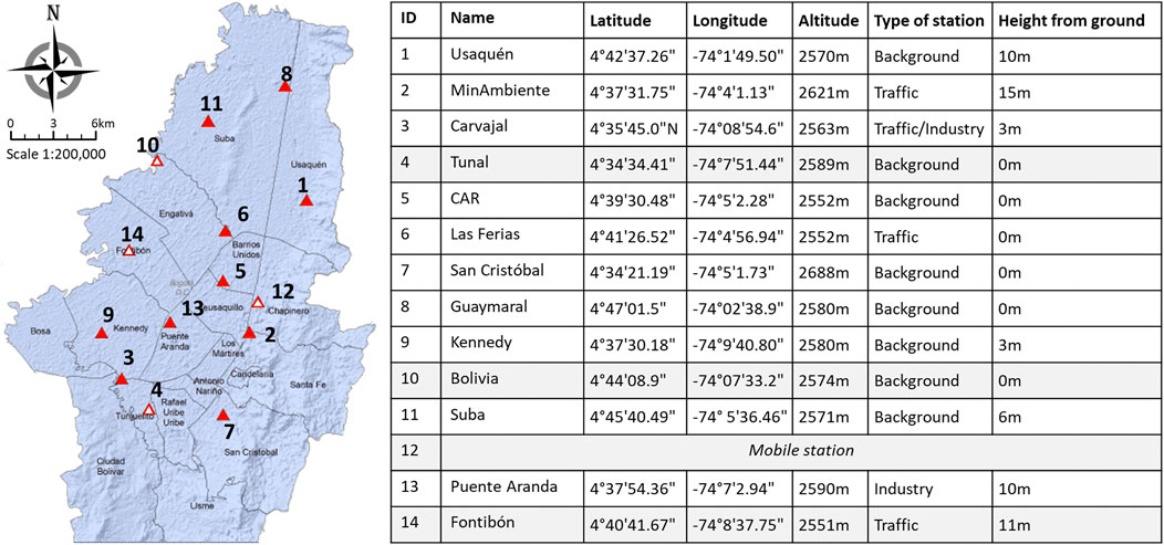
FIGURE 1. Stations of the RMCAB air quality monitoring network of Bogotá. Source: Secretaría Distrital de Ambiente, https://www.ambientebogota.gov.co/estaciones-rmcab.

According to the equipment specifications published by the Secretariat of Environment, 13 out of the 14 stations are equipped to measure and report the concentration levels of PM_2.5. For the period 2015–2018, valid PM_2.5 measurements were found available for 10 of the stations, which are those that in the map in Figure 1 are marked by solid red triangles and in the table at its right are listed with a white background.

We show in Figure 2 the box-and-whiskers plots (whiskers length equal to 1.5 interquartile ranges) of the daily average concentration of PM_2.5 measured at each monitoring station of the RMCAB. A separate plot is reported for the average daily data points of each year, from 2015 to 2018. Figure 2 also reports the guideline value set for the daily average PM_2.5 concentration by the WHO and the Colombian national standard. It can be observed that median values recorded at Carvajal, Kennedy and Puente Aranda stations exceeded the most recent WHO guideline in all the years of the considered period, other stations such as Suba and Las Ferias are showing a tendency to improvement, and the remaining ones are below the threshold. However, 6 out of the 10 stations exceed the national standard value of 50 μg/m³ (upper whiskers outside the solid line). Additionally, a large number of outlier data points, which are further above the national standard, have not been reported in the boxplot chart in Figure 2.

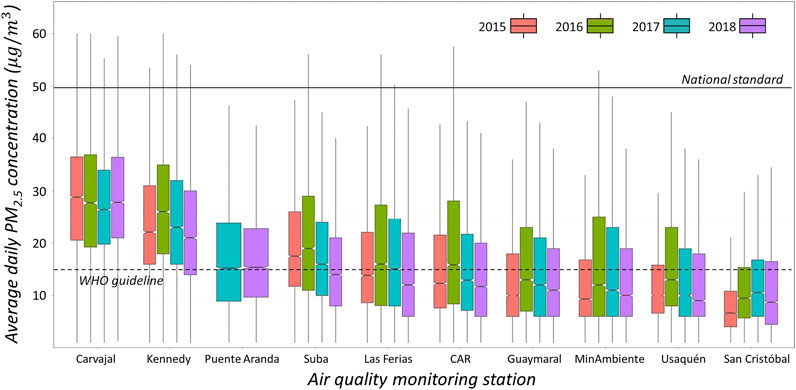
FIGURE 2. Boxplots of average daily PM_2.5 concentration measured at the RMCAB monitoring stations, from 2015 to 2018.

Here, it is important to clarify that air pollution measurements collected beyond year 2018 will not be taken into consideration in this work. We contend that 2018 was the last year for which the measurements of the RMCAB can represent historical trends in Bogotá’s air quality. In fact, as of 2019 the city began the modernization of its public transport fleet, which is still in progress. Also, the environmental authority started changing the instrumentation at some of the monitoring network stations. Finally, the city had two atypical years for traffic and industry during the COVID-19 pandemic (2020 and 2021). In our analyses, we consider the measurements from the 10 monitoring stations identified in Figure 1 as being all equally representative of the local level of exposure to PM_2.5. We acknowledge that the exact placement of the monitoring instruments determines the representativeness of the collected measurements, and that ideally, we should have used only stations whose measurements can estimate background pollutant concentration levels. On he other hand, the relationship between the type of station and the level of PM concentration measured is not so direct, and in the case of Bogotá many studies have shown that the pollutant levels reported y the monitoring stations are indeed characteristics of the geographical districts. Also, these 10 stations are routinely used by the environmental management authority to characterize the status of air quality in the city. All in all, we opted for including all these 10 stations in our analyses, ensuring that the measurements are reasonably covering the urban area of the city.

As it can be appreciated from Figure 2, air quality in Bogotá greatly varies across the city. The median daily average value of PM_2.5 concentration measured at the station of Carvajal in the south of the city is about three times the one measured in San Cristóbal (still in the south) and in Usaquén (in the north). These differences are caused by the heterogeneous distribution of emission sources such as industrial activity hot-spots and highly intensity traffic corridors, as well as the combined effect of geography and meteorological factors. Clearly, people living nearby more polluted areas, such those in the proximity of Carvajal and Kennedy monitoring stations, will be exposed to significantly poorer air quality compared to the inhabitants residing in other areas the city.

The large differences that exist among the areas of the city make clear that spatial gradients convey significant information about the state of air quality in Bogotá. While most analyses have focused on understanding how air pollution changes over time—see for instance (Mura et al., 2020), obtaining a precise picture of the impact of PM_2.5 air pollution requires taking into consideration the information about its spatial distribution. For instance, given the large differences in pollutant concentration levels across city districts, a question that naturally arises is which group of the city population is exposed to the worst/best air quality. Also, a more precise characterization of the impact could be obtained by taking into account further details about the distribution of sensitive groups (young and elder) or the possibility of getting access to health services. Answering these questions has a major practical relevance, and provides insights that could be useful for decision-makers to plan interventions and prioritizing actions aiming at reducing the deleterious consequences of poor air quality on the city dwellers.

A detailed estimation of exposure requires coupling two distinct types of information that can characterize the urban environment: the first is the spatial distribution of PM_2.5, and the second the spatial distribution of city inhabitants, disaggregated by density, age and socio-economic condition. For this to be possible, it is necessary to have available an estimation of the detailed distribution in time and space of PM_2.5 for the city. The task of obtaining the space-time field of PM_2.5 concentration from the measurements collected by the RMCAB monitoring stations will be approached in the next section, using a technique known as Kriging interpolation.

Spatial and temporal interpolation of air quality

The RMCAB stations periodically sample the PM_2.5 air pollution field across Bogotá. We deal here with the task of estimating, from the samples available at the stations, a prediction of the spatial-temporal field at any location in the geographical area of the city.

To formalize our discussion, let S denote the set of coordinates of a geographical space, and T a time interval. Also, let z(s, t) be the concentration of pollutants at location s and time t, s ∈ S, t ∈ T. Given that the topographical relief in the city of Bogotá is very limited, we model S as a subset of the 2 − dimensional Euclidean space. Let $\bar{S}=\{s_1,s_2,\dots ,s_n\}$, with s_i ∈ S, i = 1, 2, … , n be the set of locations at which the field is sampled, and $\bar{T}=\{t_1,t_2,\dots ,t_m\}$, with t_j ∈ T, j = 1, 2, … , m, be the set of sampling times. Then, for any location s ∈ S and time t ∈ T, we would like to make a reliable estimation $\widehat{z}(s,t)$ of the true value z(s, t) of the PM_2.5 concentration from the set of measured values $\{z(s_i,t_j)\mid s_i\in \bar{S},t_j\in \bar{T}\}$.

The Kriging interpolation is a family of methods in the geostatistic literature, which can be used to estimate the unknown value of a spatio-temporal field from a set of measurements collected at selected locations/times. For instance, in (Sampson et al., 2013) the authors used a regionalized universal Kriging model to estimate the annual particular matter concentration. (Song et al., 2017) resorted to ordinary Kriging and extreme learning machine to predict the concentration of soil organic matter. More recently, the work in (Shukla et al., 2020) used inverse distance weighting Kriging for particulate matter mapping, while in (van Zoest et al., 2020) a regression Kriging is adopted for modeling the urban NO₂ concentration.

The basic assumption underlying the model used for estimation in Kriging is that the correlation between values of the field decreases with the increase of distance. In this study, we choose to employ spatial temporal Kriging for interpolating the particulate matter concentration, so to take advantage of the hourly measurements taken at RMCAB stations. The dependence between distance (in time and space) and correlation is described by a function called spatial-temporal variogram. In the following sub-sections, we shall detail the specific options we consider for the variogram, and we will shortly report on the process by which we selected the Kriging interpolation approach to be used for estimating the concentration of PM_2.5 at unobserved locations/times for the city of Bogotá.

Modeling spatial-temporal variation

The most important objective when applying Kriging is to correctly capture in a model the dependence of correlation between any two points of the field and their distance. This modeling step is influenced by the assumptions that can be made on the stationarity of the field. In light of the very limited number of measurements available—only 10 locations across the whole city—we will adopt the most convenient assumptions for modeling. We believe there is no reason for trying to be overly precise when the amount of available data is so limited; rather, our objective is to obtain a reasonable approximation of the field that can serve the purpose of supporting the analyses we want to conduct in this study.

We will assume that the field z(s, t) can be modeled by a Gaussian spatial-temporal random field over S × T, and that z(s, t) can be expressed as the sum of a locally stationary mean μ(s, t) and a covariance function σ(s, t). Both components have to be estimated empirically from the available data, and the covariance part captured by a variogram γ(Δs, Δt) = σ(s₀, t₀) − σ(s, t), where Δs and Δt denote the distance in space and time. In our case, the distance between two points in space is taken to be the Euclidean distance in the flat geometry that we choose for the city of Bogotá. As for the distance in time, to take into account the existence of marked seasonality patterns (see for instance Mura et al. (2020)), we shall use a biased distance function that introduces the required periodicity.

We analyzed various possible choices of a model for the spatio-temporal variogram, i.e. those supported by the gstat package (Gräler et al., 2016) of the statistical software R (R Core Team, 2017). We observed that the simple sum metric variogram model, proposed in (Bilonick, 1988), appears to be the most flexible model. This variogram has the following form:

i.e., it is the sum of a single scalar nugget term, a spatial variogram, a temporal variogram, and a joint variogram component. In Eq. 1, 1_a denotes the indicator function, which takes the value of 1 when the predicate specified by a is true, and 0 otherwise, and κ denotes the anisotropy term, which relates the spatial variation with the temporal variations.

Each of the component variograms can be chosen independently. To determine the most suitable options, i.e. those that result in the best quality of the fitting, we conduct a comparative evaluation of a set of possible models. Specifically, we consider the spherical and Gaussian type of variogram, and fit the eight different simple sum metric models that can be obtained by the possible selection of the two options for the spatial, temporal and combined variograms. To comparatively assess the quality of the eight models, we perform a leave-one-out cross validation. Specifically, we leave out one observation $(s^{*},t^{*})\in \bar{S}\times \bar{T}$ from the input dataset for the interpolation, and we use the Kriging model to obtain the prediction $\widehat{z}(s^{*},t^{*})$ for the true (measured) value z(s*, t*) using the remaining measurements. We repeat this process for the elements in $\bar{S}\times \bar{T}$, and then we estimate a Root Mean Square Error (RMSE) for the model, as follows:

In this work, the RMSE in Eq. (2) is the metric that defines the quality of the Kriging interpolation, and the model with the minimal RMSE is the one chosen for approximating the values of the PM_2.5 field across the city. The results of the leave-one-out cross validation are reported in Table 1.

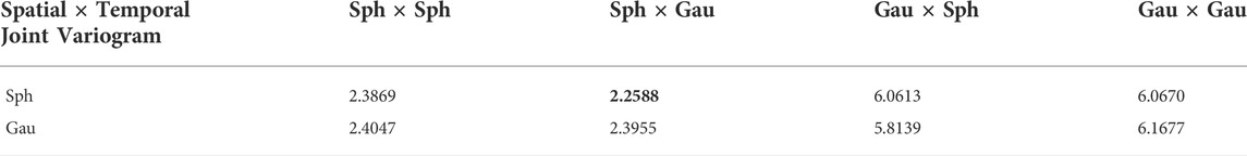
TABLE 1. RMSE obtained with the leave-one-out accuracy estimation for the different combinations of spatial, temporal and joint variograms. The smaller the error, the better the quality of the interpolation. The best model is highlighted using bold font.

Kriging interpolation results

The objective we state for the Kriging interpolation is to construct an approximation for PM_2.5 yearly average concentration field. The input data to the process consists of the whole set of RMCAB hourly measurements for years 2017 and 2018. We first aggregated the data at the month level, obtaining 24 measurements for each of the 10 locations that report PM_2.5 concentration levels. We the estimated the eight possible models based on the simple sum metric variogram, and estimated their RMSE. The results can be seen in Table 1. With the best model, we produced a set of 12 interpolated surfaces, one for each month, with one predicted value for the geographical location of the centroid of each neighborhood in the city. Then, we averaged the 12 surfaces to obtain the yearly average estimation of PM_2.5. The predicted surface of the yearly average pollutant concentration level is reported in Figure 3, and clearly shows the existence of a PM_2.5 concentration gradient that portraits a very uneven spatial distribution of poor air quality.

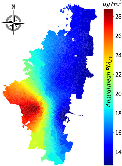
FIGURE 3. Annual ambient PM_2.5 concentration for year 2018. The spatial resolution is at the level of barrio.

Detailed descriptions of the spatial distribution of air pollutants, such as the one reported in Figure 3, allow producing more precise characterizations of PM_2.5 across the urban area. For example, it is possible to describe the exposure of city’s inhabitants at the level of the district. Figure 4 shows the distribution of the yearly average air pollutant concentration values estimated for each neighborhood (barrio, in Spanish), grouped per district. Each boxplot is drawn using the standard 1.5 inter quartile distance for the length of its whiskers. As it can be appreciated from Figure 4, the disparities among sectors of the city that were signaled by the variation among monitoring stations appear to be very relevant. The median PM_2.5 yearly concentration level (27.47 μg/m³) at the most polluted district (Tunjelito) is more than twice the median (13.18 μg/m³) of the least polluted one (Santa Fe). Moreover, three districts have a median PM_2.5 yearly concentration level beyond the national standard of 25 μg/m³. The chart in Figure 4 is an illustrative example of the insightful analyses that can be conducted using spatially distributed air pollution data.

FIGURE 4. Boxplots of the 2018 yearly average PM_2.5 concentration level for the neighborhoods of each district of the city.

Air quality and population density

As already mentioned, Bogotá is a highly heterogeneous city. Inside its boundaries, residential areas co-exist with industrial sectors, historical neighborhoods are located besides modern high-rising buildings and shantytowns where people displaced by the conflict dwell. Such a diversity gets reflected in very different densities of population across the city.

Figure 5A shows a map of the population density of the city of Bogotá in 2018 (Bogotá City Government, 2021). The data in the map is averaged at the level of the UPZ, the acronym of Unidad de Planeamiento Zonal, an intermediate level administrative sub-division between the neighborhood (barrio) and the district (localidad), and demonstrates that the variation in population density within the city boundaries is quite noticeable.

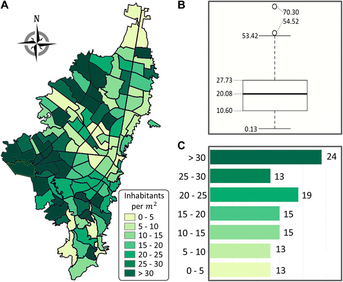
FIGURE 5. Population density across the 112 UPZs of Bogotá, in 2018. (A) map of spatial distribution of population density; (B) box-and-whiskers plot of UPZ population density values; (C) histogram of frequencies for the population density distribution across UPZs.

The range of values of the density is shown in the box-and-whiskers plot in Figure 5B, and covers an interval of values from 0.13 in the northernmost UPZ of the city, up to 50 and until 70 inhabitants/m² in the westernmost ones. Such extreme values of population density are comparable to those observed in the most dense urban areas of the world. Figure 5C provides an histogram of the population density distribution, which shows that both tails hold significant parts of the distribution.

Such differences make it more complicated to grasp a detailed understanding of how poor air quality affects city residents. To assess the exposure to pollutants, it is possible to cross the information provided by the two surfaces in Figures 3, 5. In particular, for each of the neighborhoods, we can associate the resident population with the average annual PM_2.5 concentration on that area. Thus, an empirical distribution of exposure can be generated, which describes how many people are exposed to each level of PM_2.5 air pollution. Such a distribution, summarized in the pie chart reported in Figure 6, provides a very detailed picture of the impact of poor air quality in the city of Bogotá.

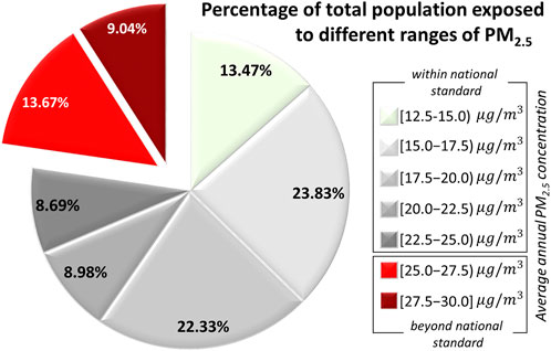
FIGURE 6. Distribution of the exposure to PM_2.5 air pollution of Bogotá residents: gray sectors for exposure to concentration below the national standard threshold, red sectors for exposure to concentrations above the threshold. Each sector reports the percentage of city residents exposed at a specific pollutant range.

Figure 6 breaks down the overall range of values of PM_2.5 concentration levels (12.5–30.0) into seven equally wide intervals. For each interval, the pie chart reports the percentage of city population that is exposed to a PM_2.5 pollution level included in the interval. The distribution in Figure 6 reveals that approximately 77.3% of the population (the part of the pie chart in shades of gray) resides in an area of the city where the average annual concentration of PM_2.5 is below the national standard of 25 μg/m³, while the remaining 22.7% (the red-shaded part in the chart) is exposed to pollution levels that exceed the norm. This latter percentage accounts for approximately 1.6 millions of the inhabitants of the city in 2018. It is also worthwhile noticing that only 13.47% of the population resides in areas with an average annual concentration of PM_2.5 below the most recent WHO recommended threshold of 15 μg/m³.

Considering the significant differences that exist in the PM_2.5 air pollution level across the city, we conduct a further analysis to better characterize the exposure. We divided the city in 3 contiguous geographical regions, characterized by similar levels of air quality. To identify the regions, we used the k-means clustering algorithm (implementation of the Scikit-learn module of Python Pedregosa et al. (2011)). The input to the clustering is a set of 3-dimensional points, each one formed by the two geographical coordinates of the center of a neighborhood, plus the concentration of PM_2.5 estimated at that location. Each input variable is pre-processed with a min-max scaling to be normalized in the [0, 1] interval.

Clustering results are reported in Figure 7, in the 3-dimensional chart shown at the left (chart A). The city area is partitioned in three regions, shown in different shades of gray on the horizontal plane, which approximately correspond to the northern, south-western and south-eastern parts of the city. On top of the clustered regions, we render the surface of PM_2.5 air pollution. As it can be observed, the southwestern cluster clearly corresponds to the most polluted part of the city, which lays under the orange-red colored area of the pollution surface. The northern and southeastern clusters are covering less polluted regions of the city.

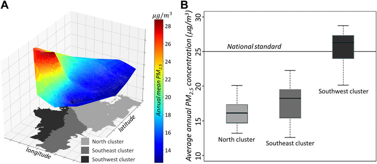
FIGURE 7. (A) on the horizontal plane the 3 clustered regions, in different shades of gray. On top, the 3-dimensional rendering of the PM_2.5 air pollution surface. (B) boxplots of PM_2.5 concentration per cluster, whiskers at 1.5 interquartile ranges.

A description of the differences in PM_2.5 concentration level among clusters is reported by the boxplots in part B of Figure 7 (right side). In each boxplot, the maximum whisker length is set to be equal to 1.5 times the interquartile range. By construction, clusters have minimal inner variance and there are no outlier values in the distributions. Thus, for each of the clusters, the whisker extreme points correspond to the extreme values of the range of PM_2.5 concentration. As it can be appreciated, each cluster has a different median value of the air pollutant concentration: 16.1 μg/m³ for the northern cluster, 18.2 μg/m³ for the southeastern one, and finally 26.3 μg/m³ for the southwestern cluster. The last cluster is significantly more polluted: all PM_2.5 values exceeding the national norm of 25 μg/m³ are grouped in this cluster.

To better quantify the contribution of each cluster to the overall exposure at the city level, we report in Figure 8 a stacked histogram chart. In this chart, the average annual PM_2.5 concentration is on the horizontal axis, and each bar shows the percentages of the city residents that are exposed to a particular level of the pollutant, broken down at the cluster level. The southwestern cluster is the only contributor to exposures above the national limit set for PM_2.5. As indicated in Figure 8, approximately 64.6% of the people resident in this cluster are exposed to pollutant concentrations beyond the acceptable values. This 64.6% corresponds to the 1.6 million city inhabitants who experience inadequate air quality conditions. This fraction of the city population is concentrated in a limited geographical area.

FIGURE 8. Detailed contribution of each cluster to the PM_2.5 air pollution exposure.

Socio-economic condition and exposure to air-quality

Many different indicators of socio-economic condition can be obtained for a population. Income and education level are two commonly used ones. In the case of Bogotá, a stratum is officially associated to each block of the city, which describes the quality of the buildings, including the construction materials, as well as the surrounding infrastructure and services.

Strata are numbered from 1, i.e., very low quality of living conditions, to 6, i.e., high, with stratum four corresponding to medium. Blocks in stratum 1 typically have major issues with the quality of the infrastructure and the provision of public services, are located in areas where construction is difficult or risky (hills, river banks), streets are unpaved, and buildings may have bare brick or even wooden walls. Stratum 6 blocks consist by large modern condos, luxurious and historical houses with gardens or in parks, usually located on panoramic locations.

Even if it is not directly determined by the income of the people living in the block, the stratum is indeed a very good indicator of their socio-economic conditions. Not only does it describe the overall quality of the living environment, but also defines how dwellers will be charged for basic services such as water, gas, power supply and land telephony lines. Therefore, for the sake of the analyses conducted in this section, the stratum will be used.

The distribution of strata is very illustrative of another layer of heterogeneity in the city. The choropleth map at the left in Figure 9 shows the spatial distribution of stratum across the UPZs of the city. For each UPZ, an aggregate stratum is computed by aggregating the strata assigned to its blocks. First, a stratum is determined for each neighborhood of the UPZ, chosen as the modal value of the strata of the blocks within. Second, the population weighted average stratum of the neighborhoods is computed to determine the stratum of the UPZ shown in Figure 9. The map clearly indicates that the majority of blocks with higher strata are located in the northeastern area of the city, and that the southernmost region has a strong prevalence of strata 1 and 2.

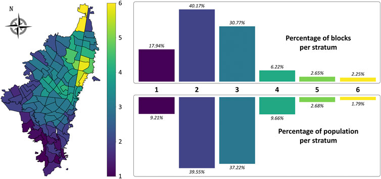
FIGURE 9. Distribution of socio-economic stratum in the city of Bogotá. At the left, spatial distribution of strata across the UPZs. At the right, overall distribution of strata across blocks and population.

The plots at the right side of Figure 9 show the strata distribution across blocks (upper bar chart), and across population (lower bar chart). As it can be seen, most blocks (approximately 89%) are categorized as pertaining to the below medium stratum (i.e., strata 1, 2, and 3). The proportion of the city population living in those strata is also similar, very close to 86%.

A side-by-side comparison of the interpolated surface for the spatial distribution of PM_2.5 concentration level in Figure 3 and the strata distribution in Figure 9 is indicative of the existence of significant disparities among the air quality levels of people living in different strata. Figure 10 shows the distribution of PM_2.5 concentration levels in each stratum (the input values for each stratum are the predicted average yearly concentrations of PM_2.5 of each neighborhood in the stratum).The difference in poor air quality exposure is immediately noticeable. The median value of the air pollutant concentration decreases with the increases of stratum, and so it does the spread of its distribution. All the low strata (1–3) have high median value, and very similar variances, with a part of the distribution exceeding the national standard of 25 μg/m³. On the other hand, the strata from medium to high (4–6) have smaller (and similar) median values, much smaller variance and all neighborhoods have average yearly PM_2.5 exposure below the national standard threshold value.

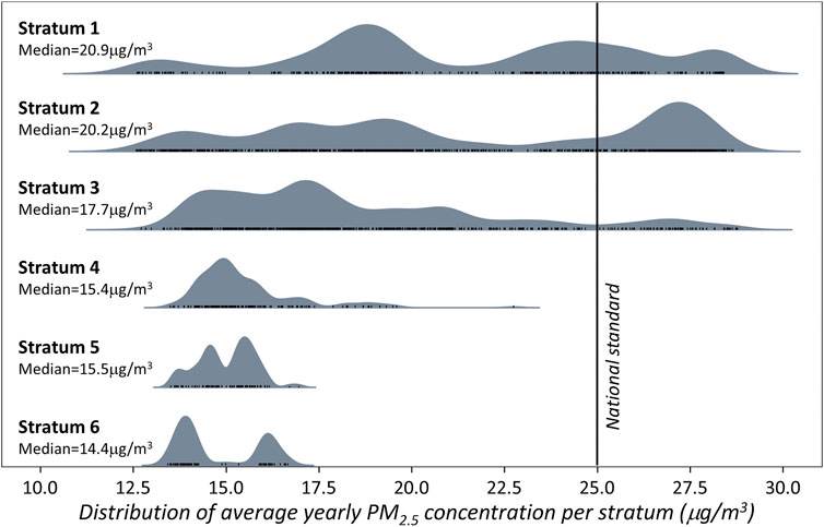
FIGURE 10. Distribution of PM_2.5 yearly average concentration per stratum. The densities are estimated with the categorical Kernel Density Estimation function of the Python Seaborn data visualization library (Waskom, 2021).

Once more, to fully understand the implications that these differences among strata have on the exposure, it is pertinent to consider the distribution of the population. As it can be appreciated from Figure 9, the city dwellers are unequally distributed across the strata. This uneven distribution adds to the disparity in exposure, because almost 86% of the population belongs to strata 1 to 3, and is thus experiencing an yearly average exposure to PM_2.5 that follows one of the three top distributions in Figure 10. This is especially important because people living in the lower socio-economic strata have limited access to high-end health services, as it has been consistently observed for in past studies, see for instance Garcia-Subirats et al. (2014); de Vries et al. (2018); Cifuentes et al. (2021). In particular, belonging to that part of the city population that receives subsidies for health services (i.e., people in strata 1 and 2) is a factor that the aforementioned research has identified as being detrimental for the overall access to health.

The map in Figure 11 shows the geographical location of all the neighborhoods whose modal stratum is either 1 or 2, and whose yearly average concentration of PM_2.5 exceeds the national standard of 25 μg/m³. To ensure the assignment of a stratum at the neighborhood level is accurate, we show besides the map in Figure 11 the distribution of blocks and population across strata. As it can be observed, only a very tiny fraction of blocks is categorized with a stratum other than 1 or 2. Those neighborhoods are all located in the southwest area of the city. They can be grouped in two clusters, which in Figure 11 are enclosed by the two rectangular regions. Clearly, the areas highlighted in Figure 11 should be object of priority interventions aimed at monitoring the health status of the citizens living therein, and ensuring that adequate health services are provided. In spite of the limited area they occupy, the 431 neighborhoods are home to more than 1.4 million people.

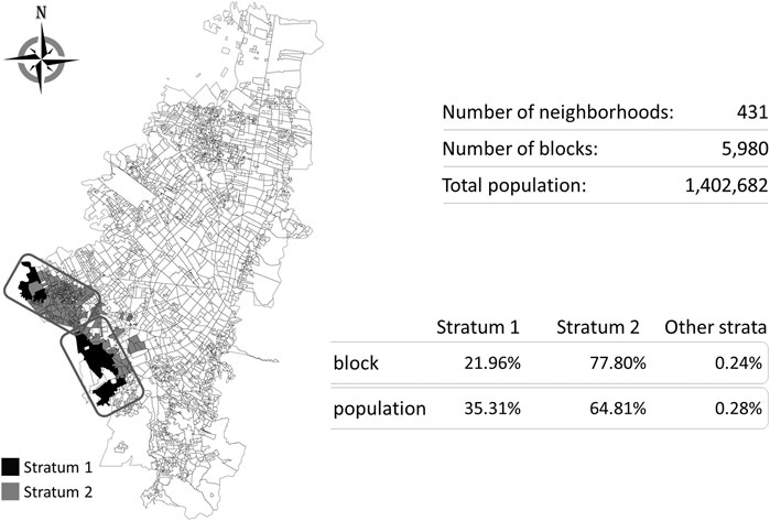
FIGURE 11. Neighborhoods of Bogotá where the yearly average PM_2.5 concentration (in 2018) exceeded the national standard threshold value, and whose inhabitants pertain to the subsided health regime.

Age group exposure to air pollution

Age is an important factor to take into consideration when evaluating the effects of air pollution. Children and elderly population are qualified as sensitive groups, and they are the first to suffer from deteriorated air quality and bear the most serious consequences (Sun and Zhu, 2019; Delgado-Saborit et al., 2021).

The differences in socio-economic conditions, and the results of recent massive urbanization waves, generate significant variations of the age distribution across the city of Bogotá. Figure 12 shows the geographical distribution of three age groups, children aged less than 5 years, young people that consists of individuals between 10 and 19 years old, and the adults older than 64 years. Note that the choropleth maps in Figure 12 are at the level of the UPZ, because that is the lowest granularity level at which the information on the age distribution is available (Bogotá City Government, 2021).

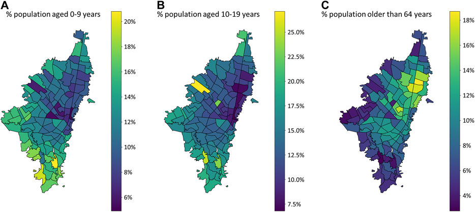
FIGURE 12. Spatial distribution of population age ranges in the city of Bogotá, at the level of the UPZ. (A) percentage of inhabitants younger than 10 years; (B) percentage of inhabitants younger than 20 years; (C) percentage of inhabitants older than 64 years.

As it can be observed from Figure 12, age has a clear gradient across Bogotá: it increases almost radially from the periphery towards the central-eastern sector that corresponds to the historical part of the city.

Given the existence of these differences in the geographical distribution of these age ranges, it is interesting to check whether they result in different exposures to air pollution, i.e., in different levels of risk for the young and the elderly. The bar diagram in Figure 13 shows the exposure to different PM_2.5 concentration ranges for two groups of the populations: children of less than 10 years, and adults older than 64 years. For each range of the pollutant and for each group, the percentage of individuals exposed is determined by their geographical distribution across the pollution field.

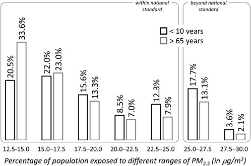
FIGURE 13. Exposure to PM_2.5 concentration of children and elderly.

Both distributions are bimodal, with a considerable part of each population group exposed to PM_2.5 concentrations above the national limit of 25 μg/m³ (21.1% of children and 15.2% of elders). However, the two age groups have different profiles of exposure, with the distribution of the children’s exposure having a larger negative skewness, which means the distribution is shifted towards the right queue. The difference is especially large for the lowest PM_2.5 concentration range, which corresponds to the best air quality conditions. Approximately one third of the adults above 64 years live in areas that enjoy this favorable conditions, while only one fifth of children under 10 years are in the same circumstances.

It is interesting to notice the similarity between the average stratum distribution at the UPZ level (left map in Figure 9) and the geographical distribution of the percentage of inhabitants aged more than 64 years (right map in Figure 12). The scatter plot of the two variables, reported in Figure 14, graphically shows the sign of a positive correlation. An adjusted R² = 0.4999 was estimated for the linear regression model. In Figure 14, the size of each bubble is proportional to the total population of the UPZ. Adding this additional piece of information shows that elderly are proportionally underrepresented in the low stratum, highly populated UPZs. On the contrary, children are proportionally less represented in high stratum, less densely populated UPZs, which are found in those areas of the city with the best air quality. Figure 15 shows the difference between the exposure of children less than 10 years old who live in stratum 1 and 2, and those of the same age who live in strata 3 to 6. The two groups have profoundly different distributions of exposure to PM_2.5. Less than 3% of children from strata three to six live in areas of the city where the average yearly concentration of PM_2.5 is above the national standard, while for children in strata one to two the percentage is ten times larger, exceeding 30%. More than 63% of children from strata three to six are living in the UPZs with the best air quality, but this percentage drops to below 9% for children from strata 1–2. It must be observed that strata one to two accounts for 30% of the children with less than 10 years in the city.

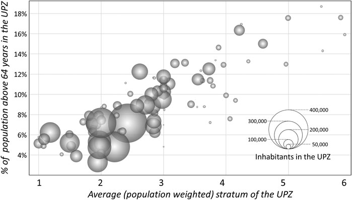
FIGURE 14. Scatter plot of the average stratum of the UPZ (horizontal axis) versus the percentage of adults older than 64 years in the UPZ.

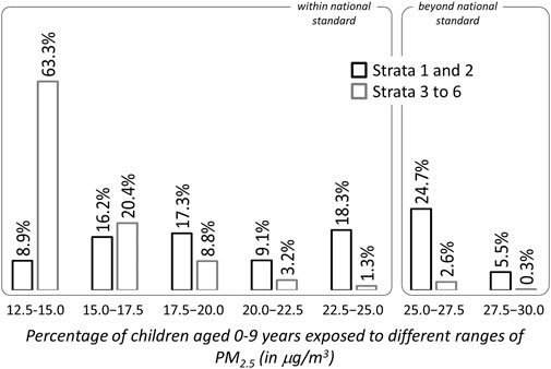
FIGURE 15. Exposure to PM_2.5 concentration for two groups of children living in different strata.

Conclusion

We propose an enriched spatial analysis of air pollution, which integrates air quality, demographic, and socio-economic data to provide decision-makers with a broader insight for urban air quality management. A significant result of this study is the recognition and quantification of profound inequities when assessing air pollution exposure, with sensitive population groups (i.e., citizens with lower income and children) being the most affected. For instance, geographical areas of the city where PM_2.5 concentrations are higher are also highly populated districts and with a greater presence of people with lower socio-economic conditions. This reality is even more critical if we take into account that Colombian air quality standards used for our analysis are significantly more permissive than the WHO guidelines.

Such findings reflect social disparities and have environmental justice implications that urge to be considered when formulating strategies to reduce air pollution and improve the living conditions of urban population. We used Bogotá, Colombia, as a study case, but the enriched spatial analysis method hereby presented is perfectly applicable to any other city in Latin America, where urban air quality is a major concern. We believe the analyses proposed in this study can provide a more comprehensive view of the impact of poor air quality, a systematic approach to assess population exposure, and a means for improving air quality management practices supporting the prioritization of air pollution abatement strategies. Future studies could consider analyzing available information on particulate spoilage chemical composition and relate its value to the presence of specific sources and risks by type of population.

Data availability statement

The datasets presented in this study can be found in online repositories available at https://gitlab.oit.duke.edu/im90/enriched-spatial-analyses-of-pm2.5.

Author contributions

All authors participated in the conceptualization of the work, in the writing and editing of the manuscript. ZJ performed the spatio-temporal Kriging, generated the visualization and participated in the analysis of results. MV conducted the original exploratory research work that led to the first draft version of the paper, including the initial Kriging, analyses and visualizations. IM supervised the whole research work, and coordinated the general revision and the update, designed the final visualizations, lead the writing and editing of the paper. JF supported the initial research, technically supervised the air quality management aspects of the paper, and contributed to the definition of analyses and interpretation of their results.

Acknowledgments

The authors acknowledge the insightful discussions held with Prof. Maria ELsa Correal at Universidad de los Andes during the inception phase of this work.

Conflict of interest

Author JF was employed by Hill Consulting, an advisory and knowledge management firm based in Colombia.

The remaining authors declare that the research was conducted in the absence of any commercial or financial relationships that could be construed as a potential conflict of interest.

Publisher’s note

All claims expressed in this article are solely those of the authors and do not necessarily represent those of their affiliated organizations, or those of the publisher, the editors and the reviewers. Any product that may be evaluated in this article, or claim that may be made by its manufacturer, is not guaranteed or endorsed by the publisher.

References

Atkinson, R., Kang, S., Anderson, H., Mills, I., and Walton, H. (2014). Epidemiological time series studies of PM2.5 and daily mortality and hospital admissions: A systematic review and meta-analysis. Thorax 69, 660–665. doi:10.1136/thoraxjnl-2013-204492
Bilonick, R. A. (1988). Monthly hydrogen ion deposition maps for the northeastern US from July 1982 to September 1984, 22, 1909–1924. doi:10.1016/0004-6981(88)90080-7Atmos. Environ.
Bogotá City Government (2022). Datos Abiertos Bogotá. Available at: https://datosabiertos.bogota.gov.co/(last time accessed: May 25, 2022).
Bogotá City Government (2021). Population for district and UPZ. Available at: https://bogota.gov.co/mi-ciudad/planeacion/visor-de-poblacion-informacion-poblacional-por-localidades-y-upz (Last time accessed: March 14, 2022).
Cifuentes, M. P., Rodriguez-Villamizar, L. A., Rojas-Botero, M. L., Alvarez-Moreno, C. A., and Fernández-Niño, J. A. (2021). Socioeconomic inequalities associated with mortality for COVID-19 in Colombia: A cohort nationwide study. J. Epidemiol. Community Health 75, 610–615. doi:10.1136/jech-2020-216275
Cohen, A. J., Brauer, M., Burnett, R., Anderson, H. R., Frostad, J., Estep, K., et al. (2017). Estimates and 25-year trends of the global burden of disease attributable to ambient air pollution: An analysis of data from the global burden of diseases study 2015. Lancet 389, 1907–1918. doi:10.1016/s0140-6736(17)30505-6
DANE (2018). Departamento administrativo nacional de estadística - censo nacional de población y vivienda. Available at: https://www.dane.gov.co/index.php/estadisticas-por-tema/demografia-y-poblacion/censo-nacional-de-poblacion-y-vivenda-2018/cuantos-somos (last accessed on June 5, 2022).
de Vries, E., Buitrago, G., Quitian, H., Wiesner, C., and Castillo, J. S. (2018). Access to cancer care in Colombia, a middle-income country with universal health coverage. J. cancer policy 15, 104–112. doi:10.1016/j.jcpo.2018.01.003
Delgado-Saborit, J. M., Guercio, V., Gowers, A. M., Shaddick, G., Fox, N. C., and Love, S. (2021). A critical review of the epidemiological evidence of effects of air pollution on dementia, cognitive function and cognitive decline in adult population. Sci. Total Environ. 757, 143734. doi:10.1016/j.scitotenv.2020.143734
Díaz, J. J., Mura, I., Franco, J. F., and Akhavan-Tabatabaei, R. (2021). aiRe-A web-based R application for simple, accessible and repeatable analysis of urban air quality data. Environ. Model. Softw. 138, 104976. doi:10.1016/j.envsoft.2021.104976
Environment Secretariat of Bogotá (2020). Informe anual de la Red de Monitoreo de Calidad de Aire de Bogotá D.C. Available at: https://oab.ambientebogota.gov.co/descargar/14112/ (last time accessed: March 27, 2022).
Environment Secretariat of Bogotá (2022). Red de monitoreo de calidad del aire de Bogotá - RMCAB, hourly reports. Available at: http://rmcab.ambientebogota.gov.co/Report/HourlyReports. (Last time accessed: March 14, 2022).
EPA (2003). Air quality index: A guide to air quality and your health. Washington DC: US Environmental Protection Agency.
Fajersztajn, L., Saldiva, P., Pereira, L. A. A., Leite, V. F., and Buehler, A. M. (2017). Short-term effects of fine particulate matter pollution on daily health events in Latin America: A systematic review and meta-analysis. Int. J. Public Health 62, 729–738. doi:10.1007/s00038-017-0960-y
Franco, J. F., Gidhagen, L., Morales, R., and Behrentz, E. (2019). Towards a better understanding of urban air quality management capabilities in Latin America. Environ. Sci. Policy 102, 43–53. doi:10.1016/j.envsci.2019.09.011
Garcia-Subirats, I., Vargas, I., Mogollón-Pérez, A. S., De Paepe, P., Da Silva, M. R. F., Unger, J. P., et al. (2014). Inequities in access to health care in different health systems: A study in municipalities of central Colombia and north-eastern Brazil. Int. J. equity health 13, 10–15. doi:10.1186/1475-9276-13-10
Gräler, B., Pebesma, E., and Heuvelink, G. (2016). Spatio-Temporal Interpolation using gstat. R J. 8, 204–218. doi:10.32614/RJ-2016-014
Hajat, A., Hsia, C., and O’Neill, M. S. (2015). Socioeconomic disparities and air pollution exposure: A global review. Curr. Environ. Health Rep. 2, 440–450. doi:10.1007/s40572-015-0069-5
Hsu, A., Reuben, A., Shindell, D., de Sherbinin, A., and Levy, M. (2013). Toward the next generation of air quality monitoring indicators. Atmos. Environ. 80, 561–570. doi:10.1016/j.atmosenv.2013.07.036
Jerrett, M., Burnett, R. T., Kanaroglou, P., Eyles, J., Finkelstein, N., Giovis, C., et al. (2001). A GIS–environmental justice analysis of particulate air pollution in Hamilton, Canada. Environ. Plan. A 33, 955–973. doi:10.1068/a33137
MinAmbiente (2008). Ministerio de Ambiente, Vivienda y Desarrollo Territorial, Protocolo para el monitoreo y seguimineto de la calidad del aire. Available at: www.minambiente.gov.co.
MinAmbiente (2017). Ministerio de Ambiente, vivienda y desarrollo territorial, resolución número 2254. Available at: https://dev.minambiente.gov.co/wp-content/uploads/2021/10/Resolucion-2254-de-2017.pdf (last accessed: may 25, 2022).
Morello-Frosch, R., Zuk, M., Jerrett, M., Shamasunder, B., and Kyle, A. D. (2011). Understanding the cumulative impacts of inequalities in environmental health: Implications for policy. Health Aff. 30, 879–887. doi:10.1377/hlthaff.2011.0153
Mura, I., Franco, J. F., Bernal, L., Melo, N., Díaz, J. J., and Akhavan-Tabatabaei, R. (2020). A decade of air quality in Bogotá: A descriptive analysis. Front. Environ. Sci. 8, 65. doi:10.3389/fenvs.2020.00065
Ouyang, W., Gao, B., Cheng, H., Hao, Z., and Wu, N. (2018). Exposure inequality assessment for PM2. 5 and the potential association with environmental health in Beijing. Sci. Total Environ. 635, 769–778. doi:10.1016/j.scitotenv.2018.04.190
Pedregosa, F., Varoquaux, G., Gramfort, A., Michel, V., Thirion, B., Grisel, O., et al. (2011). Scikit-learn: Machine learning in Python. J. Mach. Learn. Res. 12, 2825–2830. doi:10.48550/arXiv.1201.0490
Peláez, L. M. G., Santos, J. M., de Almeida Albuquerque, T. T., Reis, N. C., Andreão, W. L., and de Fátima Andrade, M. (2020). Air quality status and trends over large cities in South America. Environ. Sci. Policy 114, 422–435. doi:10.1016/j.envsci.2020.09.009
R Core Team (2017). R: A language and environment for statistical computing. Vienna, Austria: R Foundation for Statistical Computing. Available at: https://www.R-project.org/.
Sampson, P. D., Richards, M., Szpiro, A. A., Bergen, S., Sheppard, L., Larson, T. V., et al. (2013). A regionalized national universal Kriging model using partial least squares regression for estimating annual PM2.5 concentrations in epidemiology. Atmos. Environ. 75, 383–392. doi:10.1016/j.atmosenv.2013.04.015
Sheng, N., and Tang, U. W. (2016). The first official city ranking by air quality in China — a review and analysis. Cities 51, 139–149. doi:10.1016/j.cities.2015.08.012
Shukla, K., Kumar, P., Mann, G. S., and Khare, M. (2020). Mapping spatial distribution of particulate matter using Kriging and Inverse Distance Weighting at supersites of megacity Delhi. Sustain. cities Soc. 54, 101997. doi:10.1016/j.scs.2019.101997
Song, Y.-Q., Yang, L.-A., Li, B., Hu, Y.-M., Wang, A.-L., Zhou, W., et al. (2017). Spatial prediction of soil organic matter using a hybrid geostatistical model of an extreme learning machine and ordinary Kriging. Sustainability 9, 754. doi:10.3390/su9050754
Sun, Z., and Zhu, D. (2019). Exposure to outdoor air pollution and its human health outcomes: A scoping review. PloS one 14, e0216550. doi:10.1371/journal.pone.0216550
van Zoest, V., Osei, F. B., Hoek, G., and Stein, A. (2020). Spatio-temporal regression Kriging for modelling urban NO2 concentrations. Int. J. Geogr. Inf. Sci. 34, 851–865. doi:10.1080/13658816.2019.1667501
Waskom, M. L. (2021). Seaborn: Statistical data visualization. J. Open Source Softw. 6, 3021. doi:10.21105/joss.03021
World Health Organization (2021). WHO global air quality guidelines: Particulate matter (PM2.5 and PM10), ozone, nitrogen dioxide, sulfur dioxide and carbon monoxide. Available at: https://www.who.int/publications/i/item/9789240034228(last time accessed: June 5, 2022).
Keywords: air quality, PM2.5, spatial-temporal Kriging, population distribution, socio-economic conditions, sensitive groups, environmental justice
Citation: Jin Z, Velásquez Angel MA, Mura I and Franco JF (2022) Enriched spatial analysis of air pollution: Application to the city of Bogotá, Colombia. Front. Environ. Sci. 10:966560. doi: 10.3389/fenvs.2022.966560
Received: 11 June 2022; Accepted: 31 August 2022;
Published: 28 September 2022.
Edited by:
Andrew Hursthouse, University of the West of Scotland, United KingdomReviewed by:
Michael Edward Deary, Northumbria University, United KingdomSanja Potgieter, Manchester Metropolitan University, United Kingdom
Copyright © 2022 Jin, Velásquez Angel, Mura and Franco. This is an open-access article distributed under the terms of the Creative Commons Attribution License (CC BY). The use, distribution or reproduction in other forums is permitted, provided the original author(s) and the copyright owner(s) are credited and that the original publication in this journal is cited, in accordance with accepted academic practice. No use, distribution or reproduction is permitted which does not comply with these terms.
*Correspondence: Ivan Mura, ivan.mura@dukekunshan.edu.cn