Establishing a benthic macrofaunal baseline for the sandy shoreline ecosystem within the Gulf Islands National Seashore in response to the DwH oil spill

1 Introduction

As a major type of land margin feature, sandy shorelines comprise 75 percent of the coastline worldwide (Lercari and Defeo, 2003). Sandy shorelines form wherever inorganic sediments are transported to the sea by riverine discharge, distributed and deposited by longshore currents and wave action. They may stretch great distances often in conjunction with the formation of barrier island chains acting as coastal bulwarks. As such, sandy shorelines provide the first line of defense against catastrophic effects of storms and oil spills within the coastal zone (Beyer et al., 2016). Sandy shorelines provide important ecosystem services, including coastal protection, biological diversity, and trophic support of seabirds and fishes (Amaral et al., 2016; Maslo et al., 2019) as well as recreation and tourism (Klein et al., 2004; Schlacher et al., 2007; Amaral et al., 2016). However, environmental stressors increasingly threaten ecosystem services associated with sandy shorelines worldwide (Schlacher et al., 2007; Defeo et al., 2008).

Landscape-scale disturbances often afflict sandy shoreline ecosystems. Both prolonged press stressors and temporary pulse stressors (sensu Holling, 1973) influence sandy shoreline ecosystems over wide-ranging spatiotemporal scales spanning from several to thousands of km and from weeks to centuries (Defeo et al., 2008). Direct geomorphological alterations to sandy shorelines include the creation of shipping channels (Morton, 2008) which disrupt sediment transport processes (Fanini et al., 2009; Jones et al., 2011). Erosion and inundation due to storms and sea level rise due to global warming increasingly impinge upon sandy shorelines (Defeo et al., 2008). Consequently, the ecological condition and resilience of sandy shoreline ecosystems is a major concern (Jones et al., 2011).

Spatiotemporal scaling of variation in benthic macrofauna is increasingly regarded as key to understanding environmental impacts on sandy shore ecosystems (Rakocinski et al., 1998; Defeo and McLachlan, 2005; Rodil et al., 2012; Veiga et al., 2014; Pandey and Thiruchitrambalam, 2019). Morphological and behavioral adaptations have made resident macrofauna resistant to frequent natural disturbance within dynamic sandy shoreline benthic habitats (McLachlan and Jaramillo, 1995; Jones et al., 2011; Veiga et al., 2014). Thus, natural spatial patterns in sandy shoreline macrofaunal assemblages can serve as baseline indicators of excessive environmental disturbance and stress if reference conditions can be defined at the appropriate spatiotemporal scales (Bessa et al., 2013). Sandy shore macrofaunal assemblages are negatively affected at different spatiotemporal scales of impact by various stressors, including copper pollution (Arntz et al., 1987; Ramirez et al., 2005), oil contamination (Rabalais and Flint, 1983; Short et al., 2004; Owens et al., 2008), tar pollution (Shiber, 1989; Abu-Hilal and Khordagui, 2007), beach renourishment (Goldberg, 1988; Rakocinski et al., 1996; Peterson and Bishop, 2005; Jones et al., 2008; Leewis et al., 2012; Lercari and Defeo, 2003; Leewis et al., 2012; Soga and Gaston, 2018), physical structures (Kraus and McDougal, 1996; Jaramillo et al., 2002), coastal erosion (Masalu, 2002), storms and hurricanes (Rakocinski et al., 2000), and El Nino events (Castilla, 1983). Despite such studies, the spatiotemporal limits of natural variation in sandy shoreline benthic macrofauna remain poorly known (Defeo et al., 2008). Defining boundaries and threshold limits of natural macrofaunal variation within sandy shoreline ecosystems is both challenging and important.

The frequency and extent of sampling needed for defining proper baseline conditions will vary among ecosystems and biomes. Whether and how the shifting baseline syndrome (SBS) applies to defining the limits of natural variation in sandy shore macrofaunal assemblages is a primary concern (Bessa et al., 2013). The SBS refers to how background environmental degradation may elicit continuously changing reference conditions (Pauly, 1995; Soga and Gaston, 2018). The SBS problem challenges resource managers and policymakers. Unacknowledged SBS effects may confound the detection of contemporaneous macrofaunal impacts. The SBS challenge can be met by monitoring reference indicators over a sufficient time frame for detecting effects of shifting background conditions. Long-term comparisons can help determine the proper temporal scale for using monitoring data to define a dependable reference condition. Moreover, reference variation needs to be framed at the correct scale for assessing responses to different environmental stressors (Defeo and McLachlan, 2005). Greater flexibility requires more widespread and frequent sampling over longer time frames. The correct nested scale of macrofaunal variation needs to agree with the extent of exposure to the stressor of concern (Rakocinski et al., 1998).

Occurring within the northern Gulf of Mexico between April and September of 2010, the Deepwater Horizon (DwH) oil spill ranks as the biggest marine oil spill (Beyer et al., 2016). Baseline macrofaunal assemblages of sandy shoreline habitats within the Gulf Islands National Seashore (GINS) of the US National Park Service (NPS) needed to be characterized with respect to the DwH oil spill. This extensive natural sandy shoreline ecosystem offers an appropriate context for environmental assessment (Rakocinski et al., 1993; Rakocinski et al., 1996; Rakocinski et al., 1998; Rakocinski et al., 2000). A previous extensive seasonal macrofaunal inventory of the GINS in 1993 provided an operational baseline for the assessment of storm effects in 1996. However, use of the 1993 macrofaunal inventory as a baseline in the face of the 2010 DwH oil spill was questionable given the plausibility of baseline shifts over the intervening 17-year period. Notwithstanding the specialized nature of sandy shoreline macrofaunal taxa within a frequently disturbed setting, it was not known whether sandy shore assemblages were resilient enough to have completely recovered from the major large-scale hurricanes, Ivan and Katrina, occurring 5–6 years prior to the 2010 DwH oil spill. Together, these two major storms impacted both GINS districts in Florida and Mississippi. It was also essential to characterize the macrofaunal baseline with respect to the DwH oil spill at different hierarchical spatial scales corresponding to environmental factors. Thus a pre-DwH GINS macrofaunal survey was conducted right before the oil spill in spring of 2010. The 2010 pre-DwH macrofaunal survey was used to address the question of whether baseline macrofaunal assemblages shifted between 1993 and 2010 when considered at various spatial scales. For macrofaunal assemblages to serve as reliable indicators, they need to be examined within a hierarchical spatiotemporal context (Defeo and McLachlan, 2005).

To determine whether the 1993 GINS baseline was still valid, we examined hierarchical spatiotemporal scales of natural variation in macrofaunal assemblages of sandy shorelines for the combined 1993 and 2010 macrofaunal GINS datasets. We hypothesized that the 1993 GINS macrofaunal inventory baseline was stable, notwithstanding multiple disturbances by large storms within the intervening 17-year period. Additionally, the relative importance of variability in macrofaunal assemblage structure was examined across hierarchical spatial scales reflecting meaningful subdivisions of the sandy shore environment. Thus, essential scales of macrofaunal variation could be identified and validated for matching up with scales of stressor effects. Finally, a robust baseline was characterized using both datasets.

2 Study area

The US NPS Gulf lslands National Seashore (GINS) embodies natural shoreline located across two disjunct subregions separated by Mobile Bay, including a western district (i.e., Mississippi district) in Mississippi and an eastern district (i.e., Florida district) in the west Florida panhandle near the Alabama border (Figure 1). The two districts encompass land margin ecosystems including barrier islands and embayments separated by ∼ 100 km of intervening coastline. Barrier-islands include West Ship, East Ship, Horn, and Petit Bois Islands within the western Mississippi district, as well as Perdido Key and Santa Rosa Islands within the eastern Florida district. Four embayments intersecting or entirely within the GINS include Mississippi Sound in the western district, as well as smaller Big Lagoon, Santa Rosa Sound, and Pensacola Bay in the eastern district. The GINS region is influenced by major watersheds, including the Pascagoula River in the western district and the Escambia River in the eastern district. Roughly 85,000 acres of natural habitats exist within 169 km of GINS shoreline, comprising both high-energy exposed and protected medium grain quartz sand beaches, as well as adjacent grass beds and saltmarshes. Protected beaches within this region are subsidized by organic material from neighboring grassbed and salt marsh habitats.

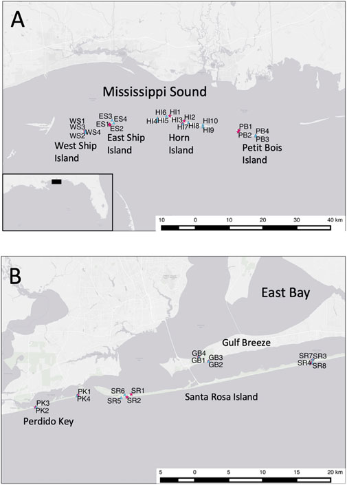
FIGURE 1. (A) Map of western district of the Gulf Islands National Seashore (GINS) study area, showing sites sampled for the 1993 macrofaunal inventory (red stars) and the 2010 macrofaunal pre-oil DwH survey (blue triangles); (B). Map of eastern district of the GINS study area, showing sites sampled for the 1993 macrofaunal inventory (red stars) and the 2010 macrofaunal pre-oil DwH survey (blue triangles).

3 Materials and methods

3.1 Field sampling

A quantitative seasonal inventory of the GINS sandy shoreline macrofauna was conducted in 1993 (Rakocinski et al., 1998). Seventeen years later, during the DwH oil spill event and before any oil impacts occurred, a pre-DwH survey of the GINS sandy shoreline macrofauna was conducted in May 2010 (Figure 1). The study design for the 2010 DwH survey was predicated on the 1993 GINS macrofaunal inventory, which comprised 148 station events including 52 collections in spring and summer, in addition to 22 station events in summer and winter. To attain a spatially balanced design for this study, the 1993 data represented spring macrofaunal samples taken from 5 April to 18 May at 51 stations among 17 sites (i.e., 10 protected, seven exposed) and the 2010 data represented samples taken from 1 May to 28 May in 2010 at 42 stations among 21 sites (i.e., 12 protected, nine exposed). In both years, at least one site was sampled from exposed and protected sites from each barrier island or mainland area where natural sandy shoreline occurred within the GINS (Figure 1). In 1993, nine sites represented the western district, including one exposed and one protected site each at West Ship Island, East Ship Island, and Petit Bois Island, as well as two protected and one exposed sites from Horn Island. Eight sites represented the eastern district in 1993, including one exposed and one protected site each from Perdido Key, two protected sites from Gulf Breeze, and two protected and two exposed sites from Santa Rosa Island. In 2010, thirteen sites represented the western district, including one exposed and one protected site each from West Ship Island, East Ship Island, and Petit Bois Island, as well as seven protected and six exposed sites from Horn Island. Eight sites represented the eastern district in 2010, including one exposed and one protected site each from Perdido Key, two protected sites from Gulf Breeze, and two protected and two exposed sites from Santa Rosa Island. Locations for many sites were similar for both surveys, but each site-event was regarded as independent, especially given the 17-year gap between the 1993 inventory and the 2010 survey. Many of our study sites were subsequently exposed to crude oil from the DwH spill.

Benthic macrofauna were sampled from the upper 20–25 cm of sediment using a 0.016 m² stainless steel box-corer (12.5 cm on a side; 1/64 m²), with the top covered by 0.5 mm stainless mesh (Saloman and Naughton 1977). In 1993, eight box-core samples were taken from each of three stations located within the intertidal swash zone, and from subtidal habitat at 5 and 15 m from the shoreline. In 2010, five box-core samples were taken from each of two stations located within the intertidal swash zone and the subtidal zone at 8 m from the shoreline. Box-core samples were spaced evenly by 1–2 m, parallel to the shoreline. Small macrofaunal organisms were removed by elutriating sediment five times through a 0.5 mm sieve using a dilute formalin solution. Remaining material was washed through a 1.0 mm sieve to recover larger heavy organisms like bivalves. This procedure is effective in removing more than 95% of the organisms (Rakocinski et al., 1991). Processed samples were labeled, fixed with 5%–10% formalin (i.e., depending on the amount of organic material), and returned to the laboratory. Collection information recorded for each event included latitude and longitude, salinity, dissolved oxygen (DO) (mg l⁻¹), pH, and water temperature (°C) at 1 m depth, as well as meteorological conditions, including wind speed and direction, tide stage, sea state, and cloud cover.

3.2 Lab processing

In the laboratory, macrofauna from each sample were sorted into major groups and transferred to 70% ethanol. Next, specimens were identified to the lowest practical taxonomic level (i.e., typically species) using existing literature and enumerated. Letters were used to represent undescribed species. A voucher collection of all nominal taxa was deposited in the USM GCRL zoology museum. A complete list of taxa for this study is presented in the Supplementary Appendix.

3.3 Data analysis

Macrofaunal community patterns and the relative importance of spatiotemporal scales of macrofaunal variation indicated by the combined 1993 and 2010 datasets were examined to define a robust baseline. Macrofaunal data represented 17 intertidal and 34 subtidal stations from 17 sites sampled in spring of the 1993 GINS inventory and 21 intertidal and 21 subtidal stations from 21 sites sampled during the 2010 DwH GINS survey. To match sampling effort at stations between 1993 and 2010, macrofaunal data were used from up to five randomly selected box-core samples for each of the 51 spring 1993 station events. The resulting data matrix for this study represented 159 macrofaunal taxa obtained from 459 box-core samples and 93 station events.

Statistical analyses were conducted using individual box-core samples, whereas some ordinations and graphical procedures were conducted at the station level, in terms of average abundances, or at the site level, in terms of centroids. Prior to calculation of Bray-Curtis dissimilarity among box-core samples or station events, macrofaunal abundances were fourth root transformed in PRIMER-e v7 to deemphasize the influence of large disparities in abundances. All macrofaunal taxa were included as 1) it is acceptable to retain rare taxa in nMDS (Anderson et al., 2008), and 2) to enable full sensitivity to the detection of baseline shifts or responses to stressors.

A preliminary station-level nMDS was used to assess macrofaunal dissimilarities among habitat zones defined by swash intertidal, 5 m subtidal, 8 m subtidal and 15 m subtidal stations. A Hierarchical Group-Average cluster analysis (Clarke and Gorley, 2015) classified station events as defined by habitat zone. Resulting group centroids were plotted for 5m, 8m, and 15 m zones along with similarity envelopes depicting group-average subdivisions superimposed within 2-D nMDS space to validate intertidal and subtidal habitat designations.

Salient macrofaunal groupings were identified from the Similarity Profile (SIMPROF) permutation procedure based on a Hierarchical Group-Average cluster analysis using an index of association for the 30 ‘most important species’ as defined by a per-sample threshold percentage in PRIMER-e 7 (Clarke and Gorley, 2015). The 30 ‘most important’ taxa were classified into eight coherent (i.e., statistically indistinguishable across all samples) indicator groups (i.e., SFGv groups) by Type 3 SIMPROF tests. Affinities of the 30 selected taxa were illustrated by plotting the relative positions of species coordinates along with their group identities within a follow-up nMDS ordination.

A Hierarchical Nested Mixed Model PERMANOVA using Type 1 sequential Sum of Squares (SS) was used to evaluate progressively inclusive sources of variation in macrofaunal dissimilarity. Type 1 SS indicates that variation attributed to specific terms in the model is exclusive and model-order-dependent. As such, successive terms explained remaining variation at larger scales, after preceding terms accounted for the smaller scales (Anderson et al., 2008). Accordingly, progressively inclusive scales ended with year as the broadest scale of variation within the hierarchically nested model. Entry order of terms into the nested mixed model followed the hierarchical arrangement of Group (box-cores for station events) as a random factor at the smallest scale, nested within habitat as a fixed factor (intertidal or subtidal), further nested within Site as a random factor, Side as a fixed factor (protected or exposed), District as a fixed factor (west or east) and terminating at the largest scale with Year as a fixed factor (1993 or 2010). Higher order interaction terms among the four fixed factors and all testable interactions involving random factors were also included within the Hierarchical Nested Mixed Model. Follow up pairwise t-tests between levels of a factor of interest within each level of an interacting factor were made for fixed factors exhibiting significant interactions within the model.

nMDS ordinations of station level or site level means in PRIMER-e v7 (Clarke and Gorley, 2015) illustrated differences in macrofaunal dissimilarity for combinations of factor levels. To determine whether differences in dispersions of sample coordinates contributed to between-group differences, homogeneity of multivariate dispersion (PERMDISP) tests compared deviations of sample coordinates from centroids between levels of fixed factors and their interactions in ordination space. Principal Coordinate Analysis (i.e., PCO or metric MDS) of the dissimilarity matrix of station means facilitated PERMDISP tests of homogeneity of multivariate dispersions of coordinates for groups relative to their centroids (Anderson et al., 2008). Pairwise t-tests were used to examine whether cumulative deviations from centroids differed among levels of fixed factors or interactions. Multiple comparisons among levels were corrected for family-wise error using Holm’s sequential Bonferroni method (Holm, 1979). To determine whether locations of sample coordinates differed among combined levels of the three fixed factors, District, Side, and Habitat, confidence intervals for locations of group centroids were ascertained by bootstrap resampling and plotted along with 96% confidence envelopes within nMDS ordination space (Clarke and Gorley, 2015).

To partition components of variation in macrofaunal dissimilarity exclusively among the main factors of concern, a complimentary hierarchical mixed model PERMANOVA involving crossed random factors based on unique elements and using Type 1 sequential Sum of Squares (SS) provided an implicitly nested model design (sensu Schielzeth and Nakagawa, 2013). Group (station-events) and Site served as random factors, which together with four fixed factors, Habitat, Side, District and Year, entered the model sequentially in the order of increasing scale. Unique elements within the random factors precluded complete crossing within the PERMANOVA design, resulting in the lack of interaction terms and de facto partitioning of the total variance into components attributable exclusively to the main factor terms. Total Sum of Squares was identical between this model and the hierarchical nested mixed model, however components of variation and significance levels differed between models for terms occurring in both models.

The Similarity Percentages (SIMPER) procedure in PRIMER-e v7 (Clarke and Gorley, 2015) helped identify which major taxa were driving differences among PERMANOVA factor levels. SIMPER outputs were used to interpret macrofaunal differences between years for the two districts, and between habitats of protected and exposed sites within the western and eastern districts. Resulting tables included differences between the top 20 numerically dominant taxa, or fewer if those dominant taxa provided ≥90% of the cumulative total abundance. Summary tables of abundances and percentages of total numbers for all taxa occurring within the eight combinations of District, Side and Habitat across both macrofaunal surveys were constructed, summarized, and compared in terms of sample effort, total density, species richness, and major taxonomic groups.

4 Results

A total of 47,571 macrofaunal organisms were obtained from 255 box core samples representing 51 station events at 17 sites for the spring 1993 inventory and from 204 box-core samples representing 42 station events at 21 sites for the spring 2010 pre-impact DwH survey. Taxonomic classification, numbers of specimens, and percent total number for all macrofaunal taxa occurring among eight combined levels of District, Side, and Habitat are presented in Supplementary Appendix S1A–S1H. The baseline dataset comprised 159 taxa, including 68 polychaete, 21 amphipod, 17 bivalve, nine decapod, nine gastropod, six isopod, six cumacean, five echinoderm, five nemertean, three mysid, two tanaid and six miscellaneous taxa (Supplementary Appendix S1I). Species richness (S) per square meter varied from 16.67 to 83.33 among the eight groups representing combined levels of District, Side, and Habitat (Supplementary Appendix S1I). The number of samples ranged between 30 and 85 box-cores, and effort was proportionate with inherent taxonomic diversity across the eight subdivisions. Species richness (S) typically reached higher levels at protected sites than at exposed sites and in subtidal habitat than in intertidal habitat (Supplementary Appendix S1I). When normalized to sample area (i.e., m⁻²), S was higher within subtidal habitat at protected sites within the eastern district than within the western district (S = 83.33 vs 61.03 m⁻², respectively). In contrast, S was higher within intertidal habitat at exposed sites within the western district than within the eastern district (S = 25.0 vs 16.67 m⁻², respectively). Total density varied from 2,120.83 m⁻² to 15,254.41 m⁻², and total densities from protected and exposed subtidal habitats differed substantially and inversely between districts: subtidal densities at protected sites were more than twice as high in the western district (15,254.41 m⁻² vs 5,937.50 m⁻²); whereas subtidal densities at exposed sites were more than fivefold higher in the eastern district (13,629.17 m⁻² vs 2,523.55 m⁻²).

Intertidal and subtidal habitat designations for nMDS and PERMANOVA were confirmed by a station-level nMDS ordination for the four habitat zones as defined by seaward distance (i.e., swash, 5 m, 8 m, or 15 m). Centroids for the zones along with accompanying similarity envelopes showed that the swash zone macrofauna was uniquely different from the subtidal zones (Figure 2). Moreover, the degree of macrofaunal dissimilarity among the three subtidal zones reflected survey year more than distance from shore, as shown by grouping of the centroids for the 5 m and 15 m zones. Thus, intertidal (i.e., swash zone) and subtidal (i.e., 5 m 8 m, and 15 m) habitat designations were used for further analysis.

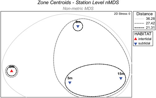
FIGURE 2. Non-metric multidimensional scaling (nMDS) centroids for station groups defined by seaward distance (i.e., swash, 5m, 8m, or 15 m) along with overlayed similarity envelopes delineated by group average cluster analysis branches.

Average total densities ranged from 1,673.75 within western exposed intertidal habitat to 15,254.41 within western protected subtidal habitat across the eight combinations of District, Side, and Habitat (Supplementary Appendix S1I). The 30 ‘most important’ taxa selected by PRIMER-e collectively made-up 94.2 percent of the total number of macrofaunal organisms. And the selected taxa formed eight coherent (i.e., statistically indistinguishable) indicator groups (i.e., SFGv groups), as determined by Type 3 SIMPROF tests (Table 1). Taxa belonging to mutually exclusive SFGv groups within nMDS space are less likely to co-occur, whereas taxa within the same groups are more likely to co-occur. These SFGv groups also likely correspond with distinct ecological conditions within the sandy nearshore environment, as illustrated by their relative positions within 2-D nMDS space (Figure 3).

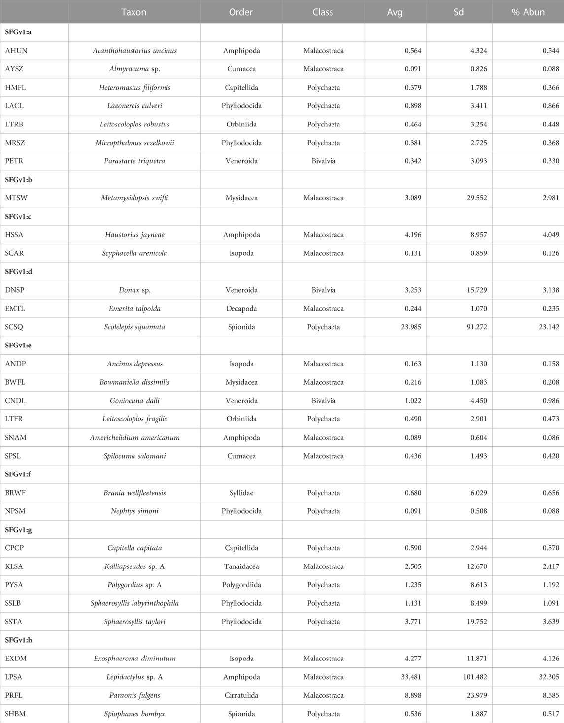
TABLE 1. Eight coherent SFGv indicator groups designated by Type 3 SIMPROF tests from among the 30 ‘most important’ taxa as selected by PRIMER-e. SFGv indicator groups exemplify co-occurring taxa. (Avg–average abundance; SD–standard deviation; % Abun–percent of total abundance; cumulative abundance for the 30 selected taxa = 94.2%.

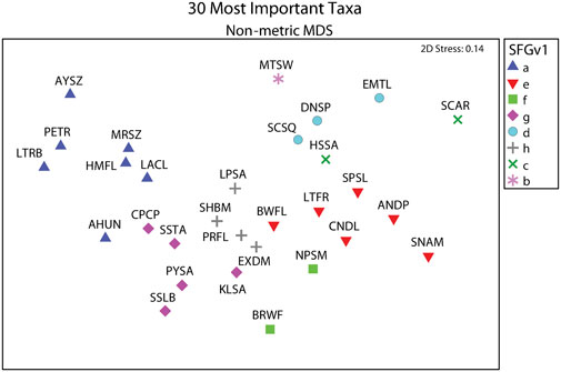
FIGURE 3. Eight coherent SFGv indicator groups designated by Type 3 SIMPROF tests from among the 30 ‘most important’ taxa selected by PRIMER-e. SFGv indicator groups exemplified co-occurring taxa as illustrated by their assigned symbols and relative positions within 2-D nMDS space. Letters in legend correspond to SFGv group identities. Specific taxa for taxon codes presented in Table 1.

The Hierarchical Nested Mixed Model PERMANOVA using Type 1 SS distinguished multiple sources of meaningful variation and effects among the 459 box-core samples (Table 2). All four of the main fixed factor terms were significant. However, the significance level of the Year main factor was comparatively weak. The Year main factor explained only 2.8 percent of the variation in faunal dissimilarity, which was the lowest of any significant effect. As the Year factor represented the highest level within the hierarchical nested model, it was given the best chance to show a difference when using the Type 1 sequential SS method, because none of the macrofaunal variation had been attributed to other factors. Accordingly, the nMDS 2-D ordination of station events showed better separation of districts than years (Figure 4A). Moreover, site centroids of station coordinates in 2-D nMDS space illustrated notable macrofaunal affinity based on island identity, regional proximity, and shore side (i.e., exposed vs protected), notwithstanding year (Figure 4B) Four two-way interactions involving fixed factors were also significant, including Year × Habitat, District × Side, District × Habitat, and Side × Habitat. In addition, the three-way District × Side × Habitat interaction was marginally significant (P = 0.036).

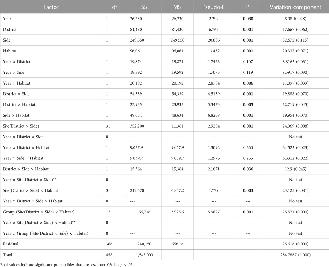
TABLE 2. Results of the Hierarchical Nested Mixed PERMANOVA using Type 1 sequential Sum of Squares. Nested factors are random. Year, District, Side, and Habitat are fixed factors, each comprising two levels. Bold–p < 0.05.

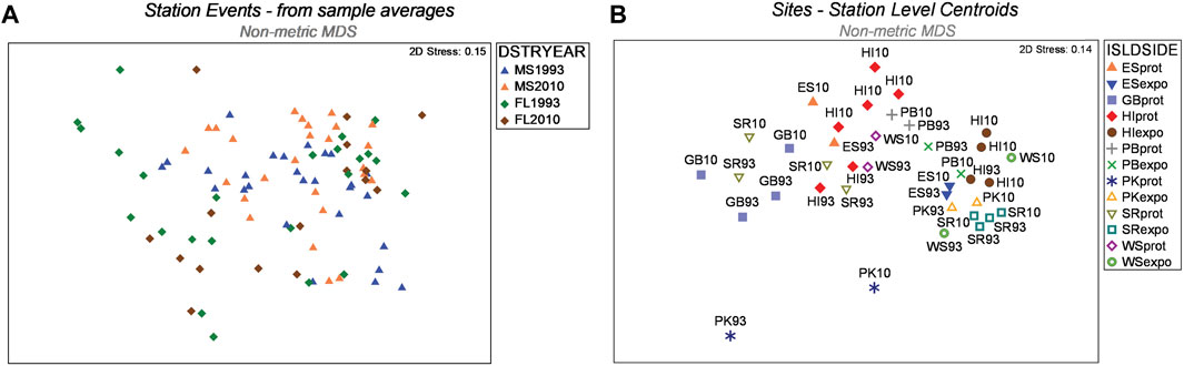
FIGURE 4. (A) Ordination of nMDS coordinates for station events. Coordinates overlap less between districts than between years (legend codes: DSTRYEAR - District/Year; MS–western district; FL eastern district; (B). Site centroids of station coordinates in 2-D nMDS space illustrating macrofaunal affinity based on island identity, region, and shore side (i.e., exposed vs protected legend codes: ISLDSIDE, Island/Side; ES, East Ship Island; GB, Gulf Breeze; HI, Horn Island; PB, Petit Bois Island; PK, Perdido Key; SR, Santa Rosa Island; WS, West Ship Island; prot, protected; expo, exposed).

When classified into eight groups representing combined levels of the three spatially hierarchical fixed factors, the nMDS 2-D ordination showed clear separation of station event groups (Figure 5A). Locations for the eight groups were clearly distinct, as shown by representative bootstrapped means and 96% confidence envelopes within nMDS space (Figure 5B). Protected sites showed greater separation within nMDS space than exposed sites. Macrofaunal dissimilarity between districts was also greater for protected sites than for exposed sites. The widest separation within nMDS space occurred between intertidal and subtidal habitats of protected sites within the Western district.

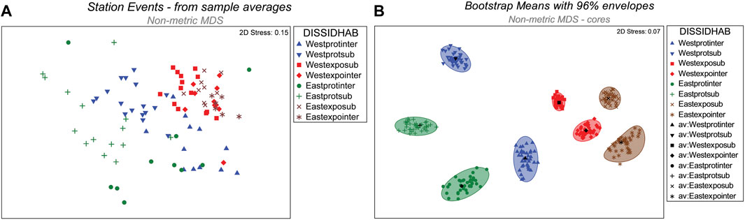
FIGURE 5. (A) Ordination of nMDS coordinates representing station events. Coordinates for the eight combinations of District, Shore side, and Habitat segregate within 2-D ordination space. (B). Plots of group centroids with 96% confidence envelopes as determined by bootstrap resampling for eight combined levels of District, Side, and Habitat. (legend codes: DISSIDHAB - District/Side/Habitat; West–western district; East -eastern district; prot–protected site; expo–exposed site; inter–intertidal habitat; sub–subtidal habitat; av, group centroid).

Follow up pairwise t-tests between factor levels of interest for significant interactions revealed that assemblages were modestly different between years within intertidal habitat, whereas assemblages were markedly different between years within subtidal habitat (Table 3). Notwithstanding between-year differences within habitats, the variance component of the Year × Habitat interaction only accounted for four percent of the total variance in assemblage structure (Table 2). Differences between the two districts as well as differences between exposed and protected sites were significant for both intertidal and subtidal habitats (Table 3; Figure 5B). And the two districts were modestly different for exposed sites and markedly different for protected sites (Table 3). Furthermore, the districts were moderately different between exposed intertidal and exposed subtidal habitats; and districts were markedly different between protected intertidal and protected subtidal habitats (Table 3; Figure 5B). Follow up differences were not of concern for significant interactions involving nested random factors. Nevertheless, significant interactions involving nested random terms collectively explained 26 percent of the variation in faunal dissimilarity (Table 2).

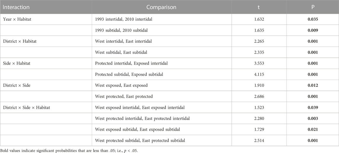
TABLE 3. Pairwise t-tests between factor levels of interest for significant interactions within the Hierarchical Nested Mixed Model PERMANOVA (Number of permutations = 998–999). Bold–p < 0.05.

In addition to locations of centroids, significant PERMANOVA results can signify differences in dispersions of nMDS coordinates between groups (Anderson et al., 2008). But PERMDISP tests of homogeneity of multivariate dispersions of nMDS coordinates were non-significant for Year (P = 0.992) and Habitat (P = 0.102) (Supplementary Appendix S2A). However, PERMDISP tests were strongly significant for District (P = 0.001) and Side (P = 0.001). Thus, both locations and dispersions of nMDS coordinates differed between both levels of the District and Side factors. Furthermore, nMDS dispersions also clearly differed among combined levels for four of six possible interactions between two fixed factors, specifically for Year by Habitat (P = 0.003), District by Side (P = 0.001), District by Habitat (P = 0.001), and Side by Habitat (P = 0.001). And dispersions differed for the three-factor combination of District by Side by Habitat (P = 0.001) (Supplementary Appendix S2A). Follow up pairwise t-tests showed that dispersions for subtidal habitat differed between 1993 and 2010 (P = 0.008), and dispersions in 2010 differed between intertidal and subtidal habitat. Salient differences in dispersions among the four combinations of District and Side included that between exposed sites of Western vs Eastern districts (P = 0.004). Salient differences in dispersions among the four combinations of District and Habitat included that for subtidal habitats of Western vs Eastern districts (P = 0.001). Salient differences in dispersions among the four combinations of Side and Habitat included that for intertidal habitats of protected vs exposed sites (P = 0.001), and for subtidal habitats of protected vs exposed sites (P = 0.001). Upon correction for family-wise significance, dispersions differed for eight of 28 combined levels of District, Side, and Habitat, including salient differences for subtidal habitats of protected sites between western vs eastern districts (P = 0.001) and for subtidal habitats between protected vs exposed sites within the eastern district (P = 0.001).

The Implicit Nested Mixed Model PERMANOVA using Type 1 sequential Sum of Squares partitioned variation entirely among the main factors at decreasing spatiotemporal scales (Table 4). The Total Sum of Squares was identical between the implicit nested model and the nested mixed model, however components of variation and significance levels of the terms differed between models. At the largest scale, Year was non-significant in the implicit nested model. However, all subsequent terms were strongly significant (P = 0.001). Moreover, when ranked in order of decreasing magnitude, variation components indicated: Group (Station level) > Shore Side > Site > Habitat > District > Year. Thus, the degree of variation attributable to the factor levels did not directly follow the inherent spatiotemporal hierarchy.

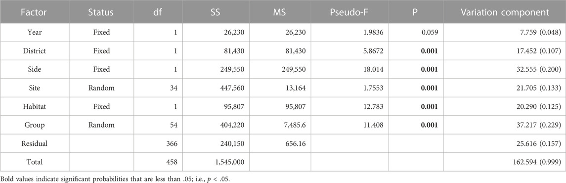
TABLE 4. Results from the Implicit Nested PERMANOVA model using a crossed design between unique coded random and fixed factors and Type 1 sequential Sum of Squares. Year, District, Side, and Habitat are fixed factors, each comprising two levels. Output terms were constrained to main factors by design, which facilitated designations of their exclusive variance components. Bold–p < 0.05.

The Similarity Percentage (SIMPER) procedure helped to interpret macrofaunal differences between years for each District and between districts for each combination of Side and Habitat (Supplementary Appendix S3A). Nine of 20 top taxa across both years were shared between districts. Of the top 20 taxa in the western district, eight taxa were more abundant in 1993 and five taxa were more abundant in 2010, whereas of the 20 top taxa in the eastern district, 13 taxa were more abundant in 1993 and five taxa were more abundant in 2010. The most dominant taxon, Scolelepis squamata, was markedly more abundant in 2010 than in 1993 in the eastern district, whereas the abundance of this polychaete was more similar between years within the western district. Conversely, the haustoriid amphipod, Lepidactylus sp. A, was more abundant in 1993 than in 2010 in both districts. Another haustoriid amphipod, Haustorius jayneae, was more abundant in 1993 within the western district, while abundances of this amphipod were comparable between years within the eastern district. And the polychaete, Paraonis fulgens, was more abundant in 1993 in both districts.

Notable differences in abundances of the top 20 taxa across both districts occurred within intertidal and subtidal habitats of protected sites (Supplementary Appendix S3A). The top 20 numerically dominant taxa within intertidal habitat at protected sites made up 85.79 percent of the total abundance. Percent average dissimilarity of intertidal habitat at protected sites between districts was 74.20. Greater abundances of Lepidactylus sp. A occurred within intertidal habitat of protected sites within the eastern district. Conversely, greater relative abundances of Scolelepis squamata and Emerita talpoida occurred within intertidal habitat of protected sites within the western district. The top 20 numerically dominant taxa within subtidal habitat at protected sites made up 51.38 percent of the total abundance between districts. Percent average dissimilarity of subtidal habitat of protected sites between districts was 80.52. Various salient taxa were more abundant within subtidal habitats at protected sites within the western district, including Exosphaeroma diminutum, Kalliapseudes sp. A, Scolelepis squamata, Paraonis fulgens, Sphaerosyllis taylori, and Spilocuma watlingi. Conversely, Laeonereis culveri was more abundant within subtidal habitat at protected sites within the eastern district. Taxonomic classification, numbers of specimens, and percent total number for all macrofaunal taxa collected from intertidal and subtidal habitats of protected sites within both districts are presented in Supplementary Appendix S1A, B, E, F.

The top 13 numerically dominant taxa within intertidal habitat at exposed sites made up 90.39 percent of the total abundance (Supplementary Appendix S3A). Percent average dissimilarity of intertidal habitat at exposed sites between districts was 47.56. Six of the 13 dominant taxa occurred exclusively within one district, five of which occurred solely within the western district. Most notably, the diminutive brooding bivalve, Goniocuna dalli, was abundant within intertidal habitat of exposed beaches within the western district, while absent from the eastern district. Conversely, the anomuran crab, Emerita talpoida, was more abundant within intertidal habitat of exposed beaches within the eastern district than in the same habitat within the western district. The top 20 numerically dominant taxa within subtidal habitat at exposed sites made up 84.24 percent of the total abundance (Supplementary Appendix S3A). Percent average dissimilarity of subtidal habitat at exposed sites between districts was 58.15. Nine of the 20 dominant taxa occurred exclusively within one district, seven of which occurred solely within the western district. Four of the salient taxa, including Paraonis fulgens, Haustorius jayneae, Ancinus depressus, and Leitoscoloplos fragilis, were more abundant within the subtidal habitat of exposed beaches within the western district, whereas four other salient taxa, including Scolelepis squamata, Metamysidopsis swifti, Donax sp., and Emerita talpoida were more abundant within the subtidal habitat of exposed beaches within the eastern district. Taxonomic classification, numbers of specimens, and percent total number for all macrofaunal taxa collected from intertidal and subtidal habitats of exposed sites within both districts are presented in Supplementary Appendix S1C, D, G, H.

5 Discussion

For macrofaunal assemblage structure to serve as robust indicator of environmental degradation, the boundaries of natural variation need to be defined and validated (Ysebaert and Herman, 2002). Properly defined baseline boundaries should facilitate detection of egregious macrofaunal impacts and recovery. This is especially challenging for sandy shore macrofaunal taxa that are adapted and subjected to varying degrees of natural disturbance on landscape and habitat scales (Jones et al., 2011), in addition to intermittent meteorological disturbances on regional scales (Rakocinski et al., 2000). Using sandy shore macrofauna as indicators of temporal environmental shifts, Bessa et al. (2014) inferred sustained effects of human pressures over a 10-year period at an urban beach. So, it is noteworthy that sandy shoreline macrofaunal assemblages appeared relatively stable on a 17-year temporal scale between spring 1993 and just before impingement by the DwH oil spill, in spring 2010. The Year factor within the implicit nested PERMANOVA model explained only 4.8 percent of the variation in faunal dissimilarity, compared to other main factors which collectively accounted for an additional 79.5 percent of the variation. Indeed, statistically indistinguishable dispersions of nMDS coordinates between spring 1993 and 2010 also confirm the lack of a substantial macrofaunal baseline shift over the 17-year intervening period. A significant Year by Habitat interaction within the hierarchical nested mixed model PERMANOVA denoted between year differences in both locations and dispersions of sample coordinates for subtidal habitat, and likely reflected the broader range of seaward distances for samples from subtidal habitat in 1993 (i.e., 5m and 15 m) than in 2010 (i.e., 8 m). Hence our combined dataset expanded baseline boundaries of natural variation in the sandy shore macrofaunal assemblage structure. Accordingly, the combined GINS data for 1993 and 2010 provide a robust baseline for natural sandy shore habitat within this region.

The lack of a major baseline shift in macrofaunal assemblage dissimilarity between 1993 and 2010 was notable given the history of disturbances by major storms within the intervening 17-year period. Most notably, two of the most severe hurricanes within the region impinged on our study area 5–6 years prior to 2010. Hurricane Ivan directly impacted the eastern district of GINS in 2004 and hurricane Katrina directly impacted the western district in 2005. Effects of hurricanes on sandy shore macrofauna have been documented within the northern Gulf of Mexico region, including the GINS (Saloman and Naughton, 1977; Rakocinski et al., 2000). Fall samples from the eastern district of our 1993 GINS inventory provided a baseline for comparing with macrofaunal samples taken in 1996, 1 year after hurricanes Opal and Erin consecutively struck in 1995 (Rakocinski et al., 2000). Effects on macrofaunal species richness, total density, densities of indicator species, and assemblage structure were still evident in fall 1996. Moreover, the degree of inferred impact corresponded with the proximity of storm disturbance on a landscape scale. Such a correspondence between macrofaunal impact and disturbance could indicate major effects of over washed sediments. The recovery of impacted shoreline macrofaunal assemblages also corresponds to landscape and habitat scale factors related to the frequency and magnitude of exposure to disruptive hydrology. Accordingly, assemblages of organisms adapted to withstand wave swept conditions, such as those populating exposed sandy shorelines and intertidal habitats, are quite resilient (Rakocinski et al., 2000). Essentially comparable macrofaunal assemblages between 1993 and 2010 implies that the sandy shore macrofauna can fully recover from regional effects of major storms within 5–6 years within our study area. Fortuitously, the 1993 GINS macrofaunal inventory provided an excellent foundation for establishing a baseline, because there had been a preceding period of 20 years without direct impacts of major storms within either district (https://www.nhc.noaa.gov/outreach/history/).

Another strong indication of an inherently stable sandy shoreline macrofauna was evinced by centroids for sites representing specific islands. Although replication was insufficient to include island as a hierarchical level within PERMANOVAs, notable fidelity in macrofaunal assemblage composition was implied by the proximity of site centroids representing specific islands in nMDS space, despite any between-year differences. High site-specific macrofaunal similarity within the 15-m subtidal zone was also apparent in a former study within this system (Rakocinski et al., 1998), for which site level fidelity in macrofaunal similarity was noted over a six- or 7-year period. In the present study, site level fidelity in macrofaunal similarity was inferred across a much longer 17-year period. More variable centroids in nMDS space for protected sites than for exposed sites reflected differences in inherent assemblage diversity. Nevertheless, the relatively close placement of centroids for proximate protected sites across the 17-year period also revealed location-specific macrofaunal fidelity. Characteristic environmental factors related to morphodynamics, as well as to physical abiotic and biotic conditions likely favored many of the same macrofaunal taxa between the two time periods (Bae et al., 2018).

The Implicit Nested Mixed Model PERMANOVA facilitated the partitioning of variance in macrofaunal dissimilarity among the main factors representing the nesting of spatiotemporal scales. As such, decreasing amounts of variance were attributed to Group (Station level random factor), Side (Landscape level fixed factor), Site (Location level random factor), Habitat (Seaward location fixed factor), District (Region level fixed factor), and finally Year (Survey level fixed factor). The Group factor delineated subjects as represented by sets of individual box-core samples at the station level. The Type 1 sequential Sum of Squares option ensured that variance ascribed to each successive hierarchical level referred only to that which was not already explained at less inclusive levels within the model. A different approach to evaluating the influence of hierarchical factors on the same sandy shore macrofauna was taken by Rakocinski et al. (1998), based on a cluster analysis using the Group Average sorting strategy and a Principal Coordinate analysis. Based on 23 common taxa from the 15 m subtidal habitat obtained in 1986/87 and 1993, the sequence of factors influencing macrofaunal similarity was Side (Landscape), followed by District (Region), Year (1986/87 vs 1993), Site (Location), and Season (spring, summer, autumn, winter). Our present study calculated dissimilarity on the entire macrofauna, included intertidal in addition to subtidal habitat, and only contained samples taken during the spring season. Despite these and other incommensurate differences between studies, the order of three major sources of macrofaunal variation ranked the same. In both studies, Side explained more variation than District, which explained more than Year. Thus, the landscape scale was more important than region, and year was the least important explanatory factor of those in common within both studies. The hierarchical placement of Season could not be compared, as only the spring 1993 samples were commensurate with 2010 pre DwH samples. But as season was the least important level noted by Rakocinski et al. (1998), data from all four seasons of the 1993 GINS inventory can also be considered as part of the valid baseline. Indeed, the subordinate role of season as a source of macrofaunal variation was noted in Rakocinski et al. (1998): “… dominant taxa occurred more consistently across seasons at individual stations than across stations within any given season.” Understanding the relative importance of nested spatiotemporal scales of macrofaunal variation facilitates environmental assessments by helping to correctly match different stressors to their spatiotemporal scales of reference (Morrisey et al., 1992; Rakocinski et al., 1998; Defeo and McLachlan, 2005; Veiga et al., 2014; Pandey and Thiruchitrambalam, 2019).

An important rationale for characterizing variation in macrofaunal assemblages at multiple nested spatiotemporal scales is to appropriately match effects of stressors to ecological responses (Defeo et al., 2008). Corresponding with scales of variation in macrofaunal assemblages, effects of disturbance and stress are expressed on various scales (Defeo and McLachlan, 2005). For example, the largest spatial scale of hurricane impact is typically expressed at the district level within our study area. The regional scale of impacts from major storms is a product of several factors, including 1) the separation of the GINS districts by about 100 km of coastline encompassing the Mobile River and Mobile Bay estuarine system; 2) impacts focused on the right front quadrants of hurricanes; and 3) a typical hurricane impact area of around 180 km. Effects of storms will also vary relative to how disturbance is manifested at smaller scales with respect to landscape and habitat features (Rakocinski et al., 2000). Effects of the DwH oil spill were also expressed across multiple scales, including the most inclusive spatial scale covering the entire GINS study area (Nixon et al., 2016). However, actual oiling of surface sediments occurred patchily on exposed and protected beaches over several years (Owens et al., 2008; Michel et al., 2013; Clough et al., 2017). Due to the disposition of the Macondo well, Florida beaches experienced heavier oiling than Mississippi beaches (Nixon et al., 2016). And incoming oil was relatively weathered in the eastern district (Snyder et al., 2014). Thus, effects of the DwH spill on macrofaunal assemblages would have been expressed at several spatial scales for which meaningful variation was observed in this study, including habitat, landscape, and district levels. Moreover, recurrent exposure to various stages of weathered oil would have continued to affect the sandy shoreline ecosystem over multiple years. It would be insightful to know when the sandy shoreline macrofauna fully recovered from the DwH event with respect to the limits defined by this study.

Despite superficial homogeneity, sandy shoreline ecosystems comprise dynamic benthic habitats that vary seasonally, regionally, and geographically (Defeo and McLachlan, 2013). Spatial variation in sandy shoreline macrofauna has been attributed to differences in shoreline morphodynamics in connection with the degree of wave exposure and attendant sediment dynamics (Oliver et al., 1979; Shelton and Robertson, 1981; Dexter, 1983; Knott et al., 1983; McLachlan et al., 1984; Eleftheriou, 1988; Fleischack and de Freitas, 1989; Raffaelli et al., 1991; Rakocinski et al., 1991; 1993; Jaramillo and McLachlan, 1993). Landscape related variation in sandy shoreline macrofaunal assemblages corresponds with different disturbance regimes in connection with sediment properties, including sediment grain size and organic content (Defeo and McLachlan, 2005; Pandey and Thiruchitrambalam, 2019). Protected shoreline habitats may also receive high subsidies of organic input from other nearby habitats like grass beds and salt marshes (Rakocinski et al., 1998). Known scale-related patterns in sandy shore macrofaunal variability include effects of local patchiness, habitat zonation, landscape related morphodynamics, and regional discontinuities (McLachlan et al., 1993; Rakocinski et al., 1993; Rakocinski et al., 1996; Rakocinski et al., 1998). In the present study, definitive macrofaunal subdivisions were defined for each of the eight combinations of levels for the three fixed factors, District, Side, and Habitat. Subdivisions were exemplified by distinct bootstrapped mean dissimilarity and 96% confidence envelopes for each of the eight factor combinations within nMDS space. Greater separation of bootstrapped means for protected sites than for exposed sites in nMDS space reflected greater macrofaunal dissimilarities at the landscape level. Discernable baseline macrofaunal assemblages were delineated by combined levels of District, Side and Habitat. Corresponding differences in macrofaunal assemblages include rare taxa which depend on adequate sample effort to obtain. Thus, assessments of environmental impacts require properly defined references. Accordingly, a complete listing of the macrofaunal data for the eight combined levels of District, Side and Habitat, along with a summary table are provided (Supplementary Appendix S1A–I).

Sandy shoreline benthic habitats worldwide consist of comparable functional groups of macrofauna, due to the general prerequisite for adaptation to wave swept conditions, including the ability to burrow and filter-feed within moving water (Rodil et al., 2014). Consequently, benthic macrofaunal assemblages of sandy shorelines are quite resilient, and thus provide good indicators of biotic integrity in the face of catastrophic damages like those presented by the DwH oil spill. However, resource managers often avoid using shoreline macrofaunal assemblages in assessments of oil spills, because macrofauna are considered too variable to serve as reliable indicators. Indeed, published assessments of the effects of the DwH oil spill on the sandy shoreline ecosystem using macrofaunal assemblages as indicators appear deficient (Beyer et al., 2016; Clough et al., 2017). Effective management of sandy shoreline ecosystems requires the development and communication of sound research tools by scientists (Scapini and Fanini, 2011). Incorporating more integrative ecological indicators like macrofaunal assemblages would help address the need to focus on the cumulative effects of oil spills (Bjorndal et al., 2011). Using macrofauna as indicators for sandy shoreline ecosystems should be eminently tractable when responses and impacts are compared on commensurate scales. Although the present study is limited to a narrow seasonal window and infrequent sampling, it provides a spatially extensive macrofaunal reference for the sandy shoreline ecosystem of the GINS at two time points spanning a 17-year period for a region of the northern Gulf of Mexico facing multiple environmental threats (Defeo et al., 2008). In conclusion, this study validates a macrofaunal baseline reference for future assessments of environmental impacts and trends, delineation of salient spatiotemporal scales, and the management of benthic habitats within the GINS sandy shoreline ecosystem.

Data availability statement

Publicly available datasets were analyzed in this study. This data can be found here: http://www.usm.edu/gulf-coast-research-laboratory/museum-collections.php.

Author contributions

CR, RH, and SL contributed to the conceptualization and design of the study. RH, CR, and SL helped to obtain funding for the study. CR and SL supervised the project. SL, KV, and CR conducted field work to obtain samples for the 2010 and 1993 GINS macrofaunal surveys. KV managed the project, including sample processing and data entry. KV and SL verified taxonomic identifications. SL created and curated the data. CR conducted the data analyses, prepared the figures, and wrote the first draft and revision. All authors reviewed and approved the draft. This paper is dedicated to the memory of RH.

Funding

The Funding to work up, accession, and catalog macrofaunal samples from the pre-oil survey and preexisting historical samples from Perdido Key into the USM GCRL museum was provided by the National Science Foundation RAPID Program Award No. DEB-1055071. This project also supported the entry of collection records into the searchable USM GCRL museum database. Funding for the 1993 GINS macrofaunal inventory was provided by the US National Park Service - Gulf Islands National Seashore, Department of the Interior Contract No. CA-5320-8-8001.

Acknowledgments

The USM Gulf Coast Research Laboratory (GCRL) assisted by providing boat time and travel expenses in support of an emergency pre-oil macrofaunal survey from shoreline habitats of the Mississippi and Florida districts of the NPS Gulf Islands National Seashore (GINS) in May 2010. National Park Service GINS personnel helped with transporting GCRL workers to conduct field work for the pre-oil macrofaunal survey. Special thanks go to the USM graduate students and other volunteers who helped with the 2010 pre-oil DwH macrofaunal survey.

Conflict of interest

The authors declare that the research was conducted in the absence of any commercial or financial relationships that could be construed as a potential conflict of interest.

Publisher’s note

All claims expressed in this article are solely those of the authors and do not necessarily represent those of their affiliated organizations, or those of the publisher, the editors and the reviewers. Any product that may be evaluated in this article, or claim that may be made by its manufacturer, is not guaranteed or endorsed by the publisher.

Supplementary material

The Supplementary Material for this article can be found online at: https://www.frontiersin.org/articles/10.3389/fenvs.2022.951341/full#supplementary-material

References

Abu-Hilal, A. H., and Khordagui, H. K. (2007). Assessment of tar pollution on the United Arab Emirates beaches. Environ. Int. 19, 589–596. doi:10.1016/0160-4120(93)90310-e
Amaral, A. C. Z., Corte, G. N., Filho, J. S. R., Denadai, M. R., Colling, L. A., Borzone, C., et al. (2016). Brazilian sandy beaches: Characteristics, ecosystem services, impacts, knowledge and priorities. Braz. J. Oceanogr. 64, 5–16. doi:10.1590/S1679-875920160933064sp2
Anderson, M. J., Gorley, R. N., and Clarke, K. R. (2008). PERMANOVA+ for PRIMER: Guide to software and statistical methods. Plymouth, UK: PRIMER-E.
Arntz, W. E., Brey, T., Tarazona, J., and Robles, A. (1987). Changes in the structure of a shallow sandy-beach community in Peru during an El Niño event. South Afr. J. Mar. Sci. 5, 645–658. doi:10.2989/025776187784522504
Bae, H., Lee, J. H., Song, S. J., Ryu, J., Noh, J., Kwon, B. O., et al. (2018). Spatiotemporal variations in macrofaunal assemblages linked to site-specific environmental factors in two contrasting nearshore habitats. Environ. Pollut. 241, 596–606. doi:10.1016/j.envpol.2018.05.098
Bessa, F., Cunha, D., Gonçalves, S. C., and Marques, J. C. (2013). Sandy beach macrofaunal assemblages as indicators of anthropogenic impacts on coastal dunes. Ecol. Indic. 30, 196–204. doi:10.1016/j.ecolind.2013.02.022
Bessa, F., Gonçalves, S. C., Franco, J. N., André, J. N., Cunha, P. P., and Marques, J. C. (2014). Temporal changes in macrofauna as response indicator to potential human pressures on sandy beaches. Ecol. Indic. 41, 49–57. doi:10.1016/j.ecolind.2014.01.023
Beyer, J., Trannum, H. C., Bakke, T., Hodson, P. V., and Collier, T. K. (2016). Environmental effects of the deepwater Horizon oil spill: A review. Mar. Pollut. Bull. 110, 28–51. doi:10.1016/j.marpolbul.2016.06.027
Bjorndal, K., Bowen, B. W., Chaloupka, M., Crowder, L. B., Heppell, S. S., Jones, C. M., et al. (2011). Better science needed for restoration in the Gulf of Mexico. Science 331, 537–538. doi:10.1126/science.1199935
Castilla, J. C. (1983). Environmental impact in sandy beaches of copper mine tailings at Chañaral, Chile. Mar. Pollut. Bull. 14, 459–464. doi:10.1016/0025-326x(83)90046-2
Clough, J. S., Blancher, E. C., Park, R. A., Milroy, S. P., Graham, W. M., Rakocinski, C. F., et al. (2017). Establishing nearshore marine injuries for the Deepwater Horizon natural resource damage assessment using AQUATOX. Ecol. Model. 359, 258–268. doi:10.1016/j.ecolmodel.2017.05.028
Defeo, O., and McLachlan, A. (2013). Global patterns in sandy beach macrofauna: Species richness, abundance, biomass and body size. Geomorphology 199, 106–114. doi:10.1016/j.geomorph.2013.04.013
Defeo, O., and McLachlan, A. (2005). Patterns, processes and regulatory mechanisms in sandy beach macrofauna: a multi-scale analysis. Mar. Ecol. Prog. Ser. 295, 1–20. doi:10.3354/meps295001
Defeo, O., Schoeman, D. S., McLachlan, A., Jones, A., Schlacher, T. A., Scapini, F., et al. (2008). Threats to sandy beach ecosystems: A review. Coast. Shelf Sci. 81, 1–12. doi:10.1016/j.ecss.2008.09.022
Dexter, D. M. (1983). “Community structure of intertidal sandy beaches in New South Wales, Australia,” in Sandy beaches as ecosystems. Editors A. McLachhn, and T. Erasmus (The Hague: JunkPubl.), 461–471.
Eleftheriou, A. (1988). The intertidal fauna of sandy beaches: A survey of the east Scottish coast (No. 38). Aberdeen: Department of Agriculture &Fisheries for Scotland, Marine Laboratory.
Fanini, L., Marchetti, G. M., Scapini, F., and Defeo, O. (2009). Effects of beach nourishment and groynes building on population and community descriptors of mobile arthropodofauna. Ecol. Indic. 9, 167–178. doi:10.1016/j.ecolind.2008.03.004
Fleischack, P. C., and de Freitas, A. J. (1989). Physical parameters influencing the zonation of surfzone benthos. Estuar. Coast. Shelf Sci. 28, 517–530. doi:10.1016/0272-7714(89)90027-9
Goldberg, W. M. (1988). “Biological effects of beach restoration in south Florida: the good, the bad, and the ugly,” in Beach preservation technology 88. Problems and advancements in beach nourishment: Florida shore and beach preservation. Editor L. S. Tait (Tallahassee, FL: Association Inc.), 19–28.
Holling, C. S. (1973). Resilience and stability of ecological systems. Annu. Rev. Ecol. Syst. 4, 1–23. doi:10.1146/annurev.es.04.110173.000245
Jaramillo, E., Contreras, H., and Bollinger, A. (2002). Beach and faunal response to the construction of a seawall in a sandy beach of south Central Chile. J. Coast. Res. 18, 523–529.
Jaramillo, E., and McLachlan, A. (1993). Community and population responses of the macroinfauna to physical factors over a range of exposed sandy beaches in south-central Chile. Estuar. Coast. Shelf Sci. 37, 615–624. doi:10.1006/ecss.1993.1077
Jones, A. R., Murray, A., Lasiak, T. A., and Marsh, R. E. (2008). The effects of beach nourishment on the sandy-beach amphipod Exoediceros fossor: impact and recovery in Botany Bay, New South Wales, Australia. Mar. Ecol. 29, 28–36. doi:10.1111/j.1439-0485.2007.00197.x
Jones, A. R., Schlacher, T. A., Schoeman, D. S., Dugan, J. E., Defeo, O., Scapini, F., et al. (2011). “Sandy-beach ecosystems: Their health, resilience and management,” in Sandy beaches and coastal zone management – Proceedings of the fifth international symposium on sandy beaches, 19th-23rd october 2009, rabat, Morocco. Editor A. Bayed (Travaux de 'Institut Scientifique, Rabat, série générale), 6, 125–126.
Klein, Y. L., Osleeb, J. P., and Viola, M. R. (2004). Tourism-generated earnings in the coastal zone: a regional analysis. J. Coast. Res. 20, 1080–1088.
Knott, D. M., Calderand, D. M., and van Dolah, R. F. (1983). Macrobenthos of sandy beach and nearshore environments at Murrells Inlet, South Carolina, U.S.A. Estuar. Coast. Shelf Sci. 16, 573–590. doi:10.1016/0272-7714(83)90087-2
Kraus, N. C., and McDougal, W. G. (1996). The effects of seawalls on the beach: part 1, an updated literature review. J. Coast. Res. 12, 691–701.
Leewis, L., van Bodegom, P. M., Rozema, J., and Janssen, G. M. (2012). Does beach nourishment have long-term effects on intertidal macroinvertebrate species abundance?. Estuar. Coast. Shelf Sci. 113, 172–181. doi:10.1016/j.ecss.2012.07.021
Lercari, D., and Defeo, O. (2003). Variation of a sandy beach macrobenthic community along a human-induced environmental gradient. Estuar. Coast. Shelf Sci. 58, 17–24. doi:10.1016/S0272-7714(03)00043-X
Masalu, D. C. P. (2002). Coastal erosion and its social and environmental aspects inTanzania: a case study in illegal sand mining. Coast. Manag. 30, 347–359. doi:10.1080/089207502900255
Maslo, B., Leu, K., Pover, T., Weston, M. A., Gilby, B. L., and Schlacher, T. A. (2019). Optimizing conservation benefits for threatened beach fauna following severe natural disturbances. Sci. Total Environ. 649, 661–671. doi:10.1016/j.scitotenv.2018.08.319
McLachlan, A., Cockcroft, A. C., and Malan, D. E. (1984). Benthic faunal response to a high energy gradient. Mar. Ecol. Prog. Ser. 16, 51–63. doi:10.3354/meps016051
Mclachlan, A., Jaramillo, E., Donn, T. E., and Wessels, F. (1993). Sandy Beach Macrofauna Communities and their Control by the Physical Environment: A Geographical Comparison. J. Coast. Res. 15, 27–38.
McLachlan, A., and Jaramillo, E. (1995). Zonation on sandy beaches. Oceanogr. Mar. Biol. Annu. Rev. 33, 305–335.
Michel, J., Owens, E. H., Zengel, S., Graham, A., Nixon, Z., Allard, T., et al. (2013). Extent and degree of shoreline oiling: Deepwater Horizon Oil Spill, Gulf of Mexico, USA. PLoS ONE 8 (6), e65087. doi:10.1371/journal.pone.0065087
Morrisey, D. J., Howitt, L., Underwood, A. J., and Stark, J. S. (1992). Spatial variation in soft-sediment benthos. Mar. Ecol. Prog. Ser. 81, 197–204. doi:10.3354/meps081197
Morton, R. A. (2008). Historical changes in the Mississippi-Alabama barrier-island chain and the roles of extreme storms, sea level, and human activities. J. Coast. Res. 246, 1587–1600. doi:10.2112/07-0953.1
Nixon, Z., Zengel, S., Baker, M., Steinhoff, M., Fricano, G., Rouhani, S., et al. (2016). Shoreline oiling from the Deepwater Horizon oil spill. Mar. Pollut. Bull. 107, 170–178. doi:10.1016/j.marpolbul.2016.04.003
Oliver, J. S., Slattery, P. N., Hulberg, L. W., and Nybakken, J. W. (1979). Relationships between wave disturbance and zonation of benthic invertebrate communities along a subtidal high-energy beach in Monterey Bay, California. Fish. Bull. U.S. 78, 437354.
Owens, E. H., Taylor, E., and Humphrey, B. (2008). The persistence and character of stranded oil on coarse-sediment beaches. Mar. Pollut. Bull. 56, 14–26. doi:10.1016/j.marpolbul.2007.08.020
Pandey, V., and Thiruchitrambalam, G. (2019). Spatial and temporal variability of sandy intertidal macrobenthic communities and their relationship with environmental factors in a tropical island. Estuar. Coast. Shelf Sci. 224, 73–83. doi:10.1016/j.ecss.2019.04.045
Pauly, D. (1995). Anecdotes and the shifting baseline syndrome of fisheries. Trends Ecol. Evol. 10, 430. doi:10.1016/S0169-5347(00)89171-5
Peterson, C. H., and Bishop, M. (2005). Assessing the environmental impacts of beach nourishment. Bioscience 55, 887–896. doi:10.1641/0006-3568(2005)055[0887:ateiob]2.0.co;2
Rabalais, S. C., and Flint, R. W. (1983). IXTOC-1 effects on intertidal and subtidal infauna of south Texas Gulf beaches. Contributions Mar. Sci. 26, 23–35.
Raffaelli, D., Karakassis, I., and Galloway, A. (1991). Zonation schemes on sandy shores: a multivariate approach. J. Exp. Mar. Biol. Ecol. 148, 241–253. doi:10.1016/0022-0981(91)90085-b
Rakocinski, C. F., Heard, R. W., LeCroy, S. E., McLelland, J. A., and Simons, T. (1993). Seaward change and zonation of the sandy-shore macrofauna at Perdido Key, Florida, USA. Estuar. Coast. Shelf Sci. 36, 81–104. doi:10.1006/ecss.1993.1007
Rakocinski, C. F., Heard, R. W., LeCroy, S. E., McLelland, J. A., and Simons, T. (1996). Responses by benthic macroinvertebrate assemblages to extensive beach restoration at Perdido Key, Florida, USA. J. Coast. Res. 12, 326–353.
Rakocinski, C. F., Heard, R. W., Simons, T., and Gledhill, D. (1991). Macrobenthic associations from beaches of selected barrier islands in the northern Gulf of Mexico. Bull. Mar. Sci. 48, 689–701.
Rakocinski, C. F., LeCroy, S. E., McLelland, J. A., and Heard, R. W. (1998). Nested spatio-temporal scales of variation in sandy-shore macrobenthic community structure. Bull. Mar. Sci. 63, 343–362.
Rakocinski, C. F., LeCroy, S. E., McLelland, J. A., and Heard, R. W. (2000). Possible sustained effects of hurricanes Opal and Erin on the macrobenthos of nearshore habitats within the Gulf Islands National Seashore. Gulf Caribb. Res. 12, 19–30. doi:10.18785/gcr.1201.03
Ramirez, M., Massolo, S., Frache, R., and Correa, J. (2005). Metal speciation and environmental impact on sandy beaches due to El Salvador copper mine, Chile. Mar. Pollut. Bull. 50, 62–72. doi:10.1016/j.marpolbul.2004.08.010
Rodil, I. F., Compton, T. J., and Lastra, M. (2012). Exploring macroinvertebrate species distributions at regional and local scales across a sandy beach geographic continuum. PloSOne 7 (6), e39609. doi:10.1371/journal.pone.0039609
Rodil, I. F., Compton, T. J., and Lastra, M. (2014). Geographic variation in sandy beach macrofauna community and functional traits. Estuar. Coast. Shelf Sci. 150, 102–110. doi:10.1016/j.ecss.2013.06.019
Saloman, C. H., and Naughton, S. P. (1977). Effect of hurricane Eloise on the benthic fauna of Panama City Beach, Florida, USA. Mar. Biol. 42, 357–363. doi:10.1007/bf00402198
Scapini, F., and Fanini, L. (2011). “The role of scientists in providing formal and informal information for the definition of guidelines, regulations or management plans for sandy beaches,” in Sandy beaches and coastal zone management – Proceedings of the fifth international symposium on sandy beaches, 19th-23rd october 2009, rabat, Morocco. Editor A. Bayed (Travaux de l'Institut Scientifique, Rabat, série générale), 6, 87–94.
Schielzeth, H., and Nakagawa, S. (2013). Nested by design: model fitting and interpretation in a mixed model era. Methods Ecol. Evol. 4, 14–24. doi:10.1111/j.2041-210x.2012.00251.x
Schlacher, T. A., Dugan, J., Schoeman, D. S., Lastra, M., Jones, A., Scapini, F., et al. (2007). Sandy beaches at the brink. Divers. Distrib. 13, 556–560. doi:10.1111/j.1472-4642.2007.00363.x
Shelton, C. R., and Robertson, P. B. (1981). Community structure of intertidal macrofauna on two surf-exposed Texas sandy beaches. Bull. Mar. Sci. 31, 833–842.
Shiber, J. G. (1989). Plastic particle and tar pollution on beaches of Kuwait. Environ. Pollut. 57, 341–351. doi:10.1016/0269-7491(89)90088-2
Short, J. W., Lindeberg, M. R., Harris, P. M., Maselko, J. M., Pella, J. J., and Rice, S. D. (2004). Estimate of oil persisting on the beaches of Prince William Sound 12 years after the Exxon Valdez oil spill. Environ. Sci. Technol. 38, 19–25. doi:10.1021/es0348694
Snyder, R. A., Vestal, A., Welch, C., Barnes, G., Pelot, R., Ederington-Hagy, M., et al. (2014). PAH concentrations in Coquina (Donax spp.) on a sandy beach shoreline impacted by a marine oil spill. Mar. Pollut. Bull. 83, 87–91. doi:10.1016/j.marpolbul.2014.04.016
Soga, M., Gaston, K. J., and Welch, C. (2018). Shifting baseline syndrome: Causes, consequences, and implications. Front. Ecol. Environ. 16, 222–230. doi:10.1002/fee.1794
Veiga, P., Rubal, M., Cacabelos, E., Maldonado, C., and Sousa-Pinto, I. (2014). Spatial variability of macrobenthic zonation on exposed sandy beaches. J. Sea Res. 90, 1–9. doi:10.1016/j.seares.2014.02.009
Keywords: benthic macrofauna, sandy shoreline, ecological indicators, shifting baseline syndrome, DWH oil spill
Citation: Rakocinski CF, LeCroy SE, VanderKooy KE and Heard RW (2023) Establishing a benthic macrofaunal baseline for the sandy shoreline ecosystem within the Gulf Islands National Seashore in response to the DwH oil spill. Front. Environ. Sci. 10:951341. doi: 10.3389/fenvs.2022.951341
Received: 23 May 2022; Accepted: 20 December 2022;
Published: 10 January 2023.
Edited by:
Brian Joseph Roberts, Louisiana Universities Marine Consortium, United StatesReviewed by:
Daniel Pech, El Colegio de la Frontera Sur, MexicoAldo Cróquer, The Nature Conservancy, Dominican Republic
Copyright © 2023 Rakocinski, LeCroy, VanderKooy and Heard. This is an open-access article distributed under the terms of the Creative Commons Attribution License (CC BY). The use, distribution or reproduction in other forums is permitted, provided the original author(s) and the copyright owner(s) are credited and that the original publication in this journal is cited, in accordance with accepted academic practice. No use, distribution or reproduction is permitted which does not comply with these terms.
*Correspondence: Chet F. Rakocinski, chet.rakocinski@usm.edu
†These authors have contributed equally to this work