A comprehensive wind speed forecast correction strategy with an artificial intelligence algorithm

1 Introduction

Weather forecasting plays a profound role in daily human life as well as in economic and social activities since it is pivotal to agriculture, disaster prevention and control, power generation, etc. (Barbounis et al., 2006). As a key indicator of the weather system, wind speed forecasting has particular value to a lot of engineering applications, e.g., meaningful for wind power generation. In particular, with the development of large-scale wind farms, more and more wind power is integrated into the power grid (Yang et al., 2014), and the accuracy of wind speed directly affects the performance of wind power scheduling. However, due to the intermittence and uncertainty of wind, the high accuracy of wind speed forecasting is a challenge.

It is known that wind speed is pertinent to numerous factors, e.g., temperature, terrain, rainfall, pressure, etc., Hu et al. (2014). Inspired by this idea, the numerical weather prediction (NWP) system is a commonly used physical model for weather forecasting and wind speed forecasting (Alexiadis et al., 1998). However, this physical model is based on a meteorological system which is huge and complex, and with an experiment overhead, it is difficult to be constructed by individuals. With this drawback, the dominant proportion of existent forecast methodologies in the literature is generally data-driven models Al-Yahyai et al. (2010). As the performance of computing devices has increased dramatically in the past decades, more advanced artificial intelligence (AI) algorithms are being applied to these data-driven models for wind speed forecasing. However, conventional data-driven methods are statistical models which can achieve good accuracy in short-term prediction but have bad performance in long-term prediction due to the error accumulation problem. Physical models, e.g., NWP, could realize the large time-scale prediction, but the forecasting results are rough and low-accurate. Combining these two methods, a useful way of improving the long-term forecasting accuracy is correction modeling which utilizes statistical models to correct the results of physical models (Voyant et al., 2012). The mechanism of error correction methodologies is usually utilizing the current weather information as the input to further correct the predicted data (Wang et al., 2019). It aims to minimize the prediction errors brought by the meteorological models.

To realize a correct model with higher accuracy in wind speed forecasting, this article proposes a kind of comprehensive correction strategy based on a deep learning algorithm. Compared with the conventional models, deep learning algorithms have a better feature representation ability to improve prediction accuracy. It provides a comprehensive model, while the customized meteorological model of the local information is not needed. It can significantly reduce the workload. This article also compares the performance of NWP models with various conventional models and deep-learning models. Experimental results show that deep learning models can significantly simplify the workflow, while the prediction accuracy is satisfied.

The layouts of the other sections are organized in the following way: Section 2 demonstrates the related work of conventional methodologies in wind speed prediction. Section 3 shows the design process of the error correction for wind speed forecasting with deep learning. A case study is given to validate the functionality of the proposed method in Section 4. Section 5 concludes the whole paper and illustrates future work.

2 Related work

To increase the accuracy of wind speed forecasting, appreciable effort from academia and industry has been dedicated to the improvement of the models. Due to the intermittency and uncertainty of wind, as reported by Li (2022a), and the observation errors of the model, the prediction inevitably introduces errors, particularly under the hourly scale.

A straightforward way to reduce forecasting errors is by improving the accuracy of the prediction model. The extensively applied methods can be categorized into two types: physical models and statistical models. Similar to NWPs, a physical model requires numerous meteorological information and a physical mechanism which makes the application and modeling complicated (Maria Grazia De Giorgi et al.,2011). As mentioned earlier, multiple physical processes such as aerodynamics, thermodynamics, and hydromechanics are involved. Thus, the physical model of the meteorological system is generally complicated (Maria Grazia De Giorgi et al., 2011). Statistical models require historical data such as wind speed and time stamps to conduct the forecasting. A classical method is the persistence method which utilizes the latest measured wind speed value as the forecast basis of the next point (Buhan et al., 2016). Its major advantage is the straightforward working principle and low-computational overhead which enable it to be easy-implemented. Li (2022a) also built the model for the wind turbine generator for wind power generation forecast error correction. Various statistical learning algorithms are also applied in the wind speed forecasting industry, e.g., the autoregressive moving average (ARMA) model (Ergin Erdem, 2011) invented in the 1980s, the artificial neural network (ANN) (Li and Shi, 2010), support vector machine (SVM) (Ren et al., 2014), etc. Moreover, some hybrid methods combining several statistical learning algorithms are also proposed. Additionally, the physical model and data-driven model can also be blended to increase the accuracy of the prediction, as demonstrated in Nielsen et al. (2007).

Lima et al. (2020) compare the historical solar data with NWP model predicted results in Brazil, and they claim the predicted results have notable differences from the local data. Thus, due to prediction error existing in all forecasting methods, post-processing methods seem to be essential to correct the forecasting error. Vogelzang and Stoffelen (2011) proposed NWP model error structure functions with the scatterometer winds. Synthetic and model prediction methods are adopted. As a mighty tool for error correction, Kalman filtering has been employed in wind prediction (Wang et al., 2021; Vogelzang and Stoffelen, 2011). The machine learning technology has superiorities in regard to self-adaptive and data-driven features which enable it to be extensively applied for data post-processing of NWP. Li et al. (2021) utilized bilinear transformation and the ICEEMDAN framework for short-term wind power prediction, while spatial-temporal analysis is applied in Li (2022b).

In Sweeney et al. (2013), different combined methods for wind speed forecasting were compared for error minimization. Zjavka (2015) proposed polynomial neural networks for on-line wind speed forecast correction. The multi-site model experimental study was conducted to validate the functionality of the proposed method. Jiang and Huang (2017) utilized hybrid methods of SVM and generalized the auto-regressive conditionally heteroscedastic model to correct the prediction error. Both the accuracy and stability of the model were satisfied. Du (2019) employed an ensemble-based method that incorporates three machine learning algorithms for NWP prediction result correction. By combining the three predicted results, it can enhance the prediction accuracy. Hossain and Mahmood (2020) used a long short-term memory model for minute-level solar energy forecasting, while Yang et al. (2014) used deep learning methods for day-ahead hour-level forecasting. Tang et al. (2022) used two shallow machine learning algorithms for medium- and long-term weather forecasting. Intelligent techniques are also employed for the underground projects of the Rockburst Hazard in Ahmad et al. (2021b) and Ahmad et al. (2022) and shallow foundation on cohesion-less soils in Ahmad et al. (2021a).

3 Materials and methods

3.1 Forecasting setup

The prediction process is defined as $\bar{v}=f(.)$, where $\bar{v}$ is the predicted 10 m wind speed, and f (.) is the NWP model. The NWP models contain errors due in part to the quality of the data used to drive the model and in part to computational limitations. Some errors are systematic, and it is desired to be reduced by applying statistical post-processing methods.

The current NWP model predicts 10 m wind speed data for every 12 h over a 13–48 h period. In addition, the real measurements are collected hourly; thus, the prediction error e_t can be calculated, as given in Eq. 1, when the real measurements are collected.

where ${\bar{v}}_t$ is the NWP wind speed at time t; v_t is the measured 10 min wind speed at time t. Figure 1 shows the heat map plot of prediction errors of one location.

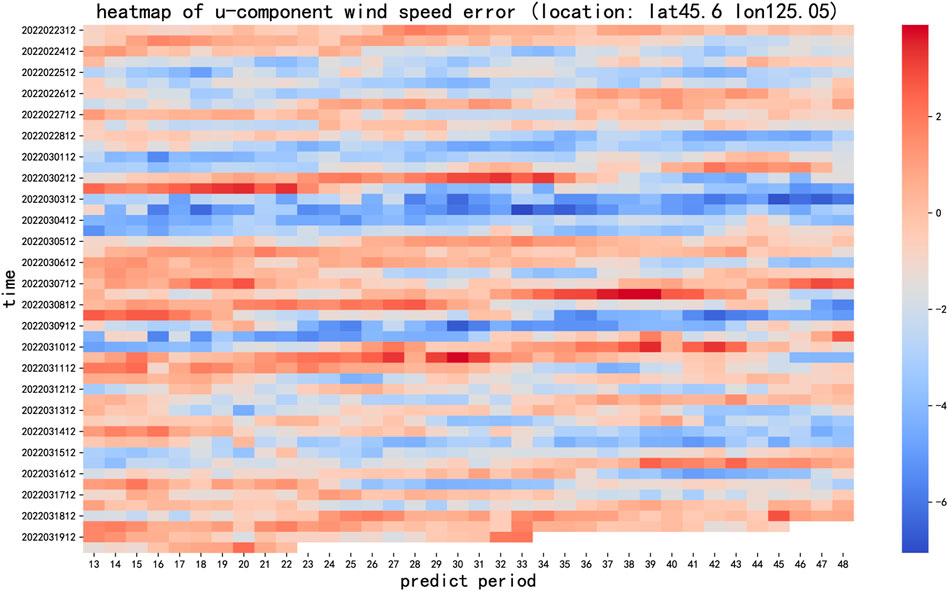
FIGURE 1. NWP prediction error of one location.

3.2 Time series-based algorithms

Time-series prediction (TSP) algorithms predict the future value over a period of time by developing models based on previous data and applying them to conduct prediction. The future is estimated based on what has already happened. Following the principle of TSP, the historical errors are learned and modeled to predict the future error, as shown in Figure 2. Once the error is predicted, the NWP wind speed can be corrected easily by just adding the predicted error. This process is expressed by Eq. 2 and Eq. 3:

where ${\widehat{e}}_t$ is the predicted error at time t and ${\widehat{v}}_t$ is the corrected NWP wind speed.

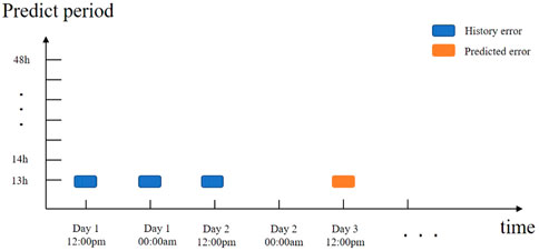
FIGURE 2. Time series prediction for correction.

3.3 Deep learning-based algorithms

TSP-based algorithms only leverage historical error information, yet other features such as temperature and air pressure, are generally neglected. Moreover, for different locations and predicted periods, TSP-based algorithms need to be modeled separately. In other words, for an NWP system monitoring 50 locations over 13–48 h periods, 1800 models are needed separately in terms of learning parameters and prediction. The modeling process is time-consuming.

To generalize the application scenarios of the forecasting model, in this paper, deep learning algorithms are utilized since they are able to automatically learn arbitrary complex mappings from inputs to outputs, which have been widely used in time series prediction tasks recently. Deep learning-based time series prediction algorithms are able to take location patterns and prediction periods into consideration and thus can train a generalized model with location patterns and prediction periods as input features. For the sake of simplicity, deep learning-based TSP algorithms are verified to pose an optimal balance among multiple parallel prediction tasks such as wind speed prediction for various locations and prediction periods.

3.3.1 Recurrent neural networks

Recurrent neural networks (RNNs) are appropriate for modeling time series data with the recurrent structure which uses neural networks to model the functional relationship between input features in the recent past to a target variable in the future.Figure 3 shows the structure of the RNN in which the transition of a hidden state from consecutive time slots is learnt from historical data. Specifically, the prediction of the output y_t depends not only on the input x_t but also on the hidden state w_ht, as shown in Eq. 4. w_ht plays the role of memorizing the previous information by weighting the previous output y_t−1. However, RNNs have the disadvantage of vanishing gradients due to the weight matrix multiplication at each time step. Thus, the RNN is not good at capturing non-stationary dependencies that occur over a long period of time.

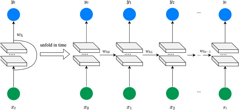
FIGURE 3. RNN model structure.

3.3.2 Long short-term memory model

The long short-term memory (LSTM) model is a variant of the RNN first, as proposed by Zjavka (2015), to overcome the gradient vanishing problem in the vanilla RNN. Figure 4 shows the structure of an LSTM cell in which a cell state c and three gates are imported to enable the storage and access of information over long periods of time. Gates are composed of a sigmoid neural net layer and a point-wise multiplication operation which are able to optionally let information through. First, the input gate weighs the current input x_t and previous output h_t−1, as shown in the following:

where W_i and b_i are the weight matrix and the bias vector of the input gate, respectively. The output of the input gate controls the selection of information in the cell state.

where W_c and b_c are the weight matrix and bias vector of the input layer, respectively. Therefore, the selected information can be represented by ${\text{c}}_t^i≔{\mathbf{i}}_t\odot {\tilde{\mathbf{c}}}_t$.

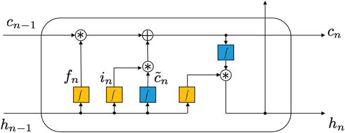
FIGURE 4. LSTM cell.

Similarly, the forget gate controls the selection of information that should be dropped:

where W_f and b_f are the weight matrix and bias vector of the forget gate, respectively. Then, the new cell state is as follows:

The output gate decides which part of information should be the output, i.e.,

where W_o and b_o are the weight matrix and bias vector of the forget gate, respectively.

4 Experimental study

In this section, the actual weather forecast data are utilized to evaluate the time series and deep learning-based strategies. The historical NWP output data are produced by Weather Research and Forecasting (WRF)-3.5 adopted by the Inner Mongolia Meteorology Bureau as one of their bases to deliver daily weather forecasts of that region. The WRF-out data are generated every 12 h (at 00:00 UTC and 12:00 UTC) from June 2019 to March 2022, containing predictions in advance of 12 h extending to 96 h with an interval of 1 h. The corresponding ground truth data are acquired from the China land surface data assimilation system, 2rd version (CLDAS-V2.0), which provide near-real-time reanalysis field data via integrating information from land surface stations, radars, and remote sensing of satellites.

The following experiments are implemented on a Linx PC with AMD Ryzen 5 3550H, 2.1 GHz CPU, 16 GB of RAM, and Python 3.8 with TenserFlow 2.8.0.

4.1 Empirical evaluation

To verify the superiority of the proposed correction strategy, the original NWP wind speed error and corrected wind speed error are compared. For the TSP-based algorithms, the training data are the past original NWP wind speed errors for a specific location and a specific prediction period. In contrast, for the deep-learning-based algorithms, the past original NWP wind speed errors for all locations and all predicted periods are used to train a general model. The input is features that are created from the historical NWP wind speed errors and additional related information.

4.1.1 Location-based evaluation

For the purpose of evaluating the correction and predicting the performance of the proposed strategy over all locations, the root mean square error (rmse) and the mean absolute error (mae) are used as the performance criteria. Obviously, the smaller the value, the better the performance of the proposed model is.

where $t\in {\mathcal{N}}^T$ is the time slot for making prediction, and $n\in {\mathcal{N}}^N$ is the prediction period. Thus, rmse_loc evaluates the overall prediction performance for location loc. Similarly,

The overall forecasting performance is evaluated in Figure 5 and Figure 6. The boxplot is used to compare the overall performance based on locations. The curve of NWP, i.e., the blue one on the left, shows the predicted results without correction. Rolling mean, ETS, and ARIMA denote the predicted results of the NWP model with conventional data correction models, while LSTM and CNN are the predicted results corrected with deep learning algorithms. From the result, without forecast correction, the rmse and mae are apparently higher than those with correction. Both TSP-based algorithms and deep-learning-based forecast correction algorithms are able to reduce the prediction error. Specifically, rolling mean methods and LSTM show the best comprehensive performance. Thus, forecast correction is necessary since it can significantly increase the prediction accuracy. However, as demonstrated earlier, the rolling mean, exponential smoothing (ETS), and autoregressive integrated moving average (ARIMA) methods all need to build the local NWP model. This means the model is no longer applicable if the location changes. The deep learning model does not need to be trained repeatedly by location patterns and predicted period data which enables it to be more universal. Also, Figure 5 and Figure 6 show that the CNN algorithm has a reduced upper limit and lower limit of RMSE over the LSTM algorithm, but the LSTM algorithm has a lower average RMSE. Reliability has the highest priority in terms of weather forecasting. Therefore, LSTM is still the most recommended algorithm for NWP forecast correction.

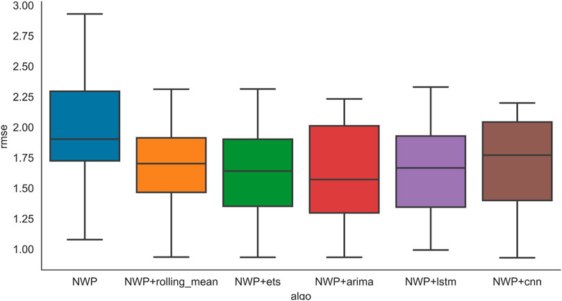
FIGURE 5. Overall rmse results based on the location.

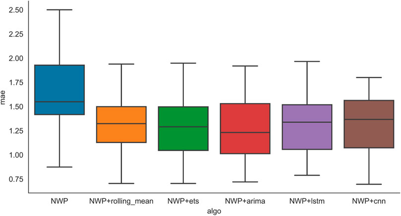
FIGURE 6. Overall mae results based on the location.

4.1.2 Prediction period-based evaluation

Similarly, rmse and mae for different prediction periods are also learnt to evaluate the correction and predicting the performance of the proposed strategies.

where $l\in {\mathcal{N}}^L$ is the location set. Thus, rmse_n and mae_n represent the overall predicting performance at the prediction period n.

To validate the application of the aforementioned algorithm in the short-term weather forecast, the predicted results over 48 h are plotted, as shown in Figures 7, 8. From the plots, without forecast correction, the rmse_n is 2.05 and the mae_n is 1.65. With forecast correction, the rmse_n is reduced to be lower than 1.7 and the mae_n is reduced to be lower than 1.4. It should be noted that the error of the CNN algorithm is high in the first 20 h and then falls down and stays stable in the following period. The NWP with the LSTM forecast correction model shows superior comprehensive performance over the other algorithms.

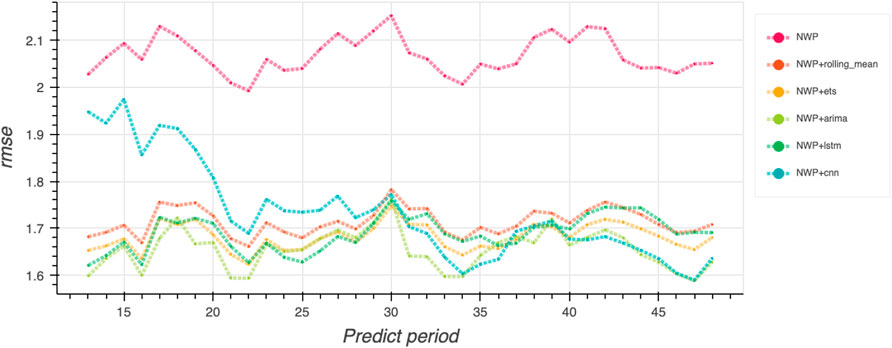
FIGURE 7. Overall rmse results based on the prediction period.

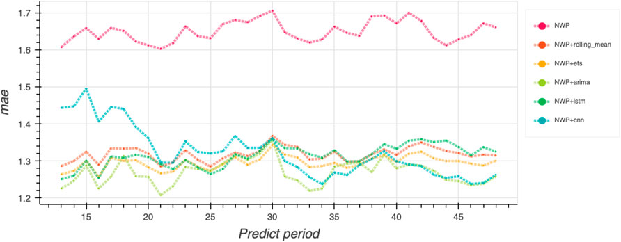
FIGURE 8. Overall mae results based on the prediction period.

4.1.3 Clustering method-based evaluation

Different locations have different geographical features, i.e., some locations are on the highland, while some may be near the waters. Instead of treating them equally, clustering them into different groups may enhance the model representation ability. To verify this, three clustering methods based on the global position system (GPS) data are used to take advantage of the geographical information. The clustering results are further input to the LSTM model as additional features. Figure 9, Figure 10 and Figure 11 show the clustering of GPS data by different algorithms, where the locations are categorized into different groups.

FIGURE 9. Clustering of the global positioning system (GPS) location by k-means.

FIGURE 10. Clustering of the GPS location by density-based spatial clustering of applications with noise (DBSCAN).

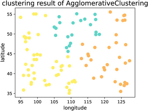
FIGURE 11. Clustering of the GPS location by agglomerative clustering.

The comparison results are shown in Figure 12 and Figure 13. From the plots, all the clustering methods can further reduce the rmse and mae. Among these clustering methods, agglomerative clustering has the best performance on reducing the rmse, while k means showed a better effect than others in terms of the mae.

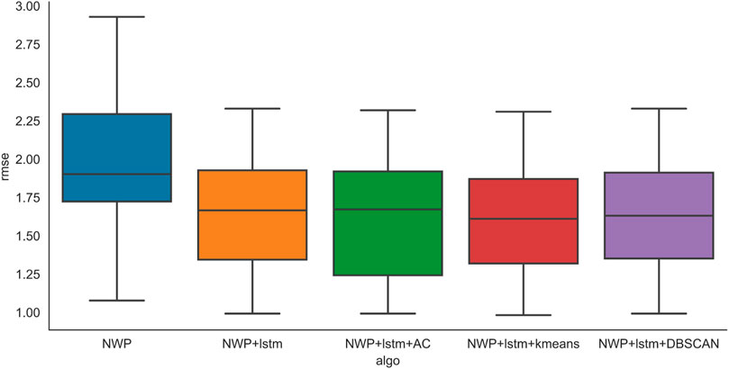
FIGURE 12. Overall rmse results for different clustering methods based on the location.

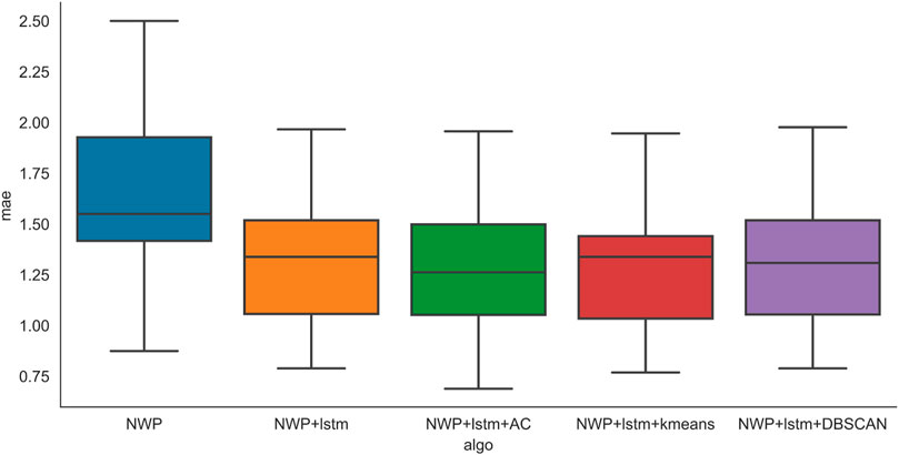
FIGURE 13. Overall mae results for different clustering methods based on the location.

4.1.4 Multi-step prediction evaluation

Previously, all results are one-step predictions, where historical data are used to predict the next time slot. In this subsection, multi-step prediction performance is learned. Figure 14 and Figure 15 show the rmse and mae results of the different step prediction performances, respectively. From the results, the predicting performance drops slightly as the prediction step increases.

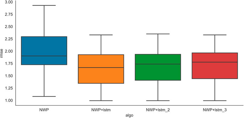
FIGURE 14. Overall rmse results for different prediction steps based on the location.

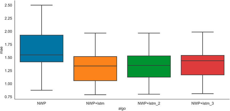
FIGURE 15. Overall mae results for different prediction steps based on the location.

5 Discussion

With the rapidly increasing demand for wind energy, the fluctuation and intermittence pose challenges to power dispatch. Thus, it is desired to have an accurate prediction of the wind speed. From the experimental results presented in Section 4, the NWP model shows considerable prediction errors, and this is also reported by Lima et al. (2020). Therefore, forecasting correction is necessary. In industry applications, how to minimize prediction error is still a major challenge. This study presents the application of deep learning algorithms on the forecasting correction for the NWP prediction results. Several conventional methodologies including rolling mean, ETS, and ARIMA are compared with deep learning methodologies such as LSTM and CNN. Both methodologies show superiority in terms of prediction accuracy enhancement. Based on the analysis demonstrated in this article, the accuracy of the wind speed prediction can be enhanced from the following perspectives.

5.1 Improved NWP model

Wind speed is an important output of the NWP model, which is utilized to describe meteorological evolution. Its accuracy can significantly increase prediction accuracy. The modeling of the local information is comprehensive progress. Generally, the accuracy of the model is impacted by multiple factors, such as the time step. However, with higher resolution, the computational load increases dramatically. Thus, the NWP model should consider the tradeoff between the computational load and accuracy.

5.2 Application of the deep learning-based error correction algorithm

From the analysis of this paper, both TSP-based and deep-learning-based error correction algorithms can effectively reduce prediction error. The experimental study shows that both methodologies can realize the same effect in terms of prediction error minimization. TSP algorithms are generally easier to be implemented when the computational load is lower. However, repeated modeling is needed if the location information changes. Also, the selection of the TSP algorithm can have a great impact on the prediction. Hence, the TSP algorithm should be estimated prior to using it.

The deep learning algorithm is data-driven, and it just needs the local weather information to train the algorithm. It can save time in mathematical modeling. Therefore, the penetration of deep learning-based methods is increasing in the industry. The experimental study is conducted to compare the accuracy of the proposed method with ARIMA, ETS, and LSTM. LSTM shows the best overall performance among the listed methods. It should be noted that clustering does not show critical improvement to prediction accuracy. However, it can increase the computational speed, which makes it still necessary.

Data availability statement

The data analyzed in this study are subject to the following licenses/restrictions: confidential meteorological data which are not published. Requests to access these datasets should be directed to sunqilong@cigit.ac.cn.

Author contributions

XZ proposed the idea and finished this article. QS provided the original data for the experimental study and wrote the code of the algorithms. WT, SY, and BW assisted in deep learning algorithm training and running the algorithm.

Funding

This work was funded partially by the Chinese Academy of Sciences (No. KFJ-STS-QYZD-2021-01-001) and the Inner Mongolia Meteorological Observatory (No. QXT21111102).

Conflict of interest

Authors WT, SY, and BW are employed by China Merchants Fintech Company Ltd.

The remaining authors declare that the research was conducted in the absence of any commercial or financial relationships that could be construed as a potential conflict of interest.

Publisher’s note

All claims expressed in this article are solely those of the authors and do not necessarily represent those of their affiliated organizations, or those of the publisher, the editors, and the reviewers. Any product that may be evaluated in this article, or claim that may be made by its manufacturer, is not guaranteed or endorsed by the publisher.

References

Ahmad, M., Ahmad, F., Wróblewski, P., Al-Mansob, R. A., Olczak, P., Kamiński, P., et al. (2021a). Prediction of ultimate bearing capacity of shallow foundations on cohesionless soils: A Gaussian process regression approach. Appl. Sci. 11, 10317. doi:10.3390/app112110317
Ahmad, M., Hu, J.-L., Hadzima-Nyarko, M., Ahmad, F., Tang, X.-W., Ur Rahman, Z., et al. (2021b). Rockburst hazard prediction in underground projects using two intelligent classification techniques: A comparative study. Symmetry 13, 632. doi:10.3390/sym13040632
Ahmad, M., Katman, H. Y., Al-Mansob, A. F., Ramez, A., Safdar, M., and Alguno, A. C. (2022). Prediction of rockburst intensity grade in deep underground excavation using adaptive boosting classifier. Complexity 2022, 1–10. doi:10.1155/2022/6156210
Al-Yahyai, S., Charabi, Y., and Gastli, A. (2010). Review of the use of numerical weather prediction (nwp) models for wind energy assessment. Renew. Sustain. Energy Rev. 14, 3192–3198. doi:10.1016/j.rser.2010.07.001
Alexiadis, M., Dokopoulos, P., Sahsamanoglou, H., and Manousaridisa, I. (1998). Short term forecasting of wind speed and related electrical power. Sol. Energy 63, 61–68. doi:10.1016/S0038-092X(98)00032-2
Barbounis, T., Theocharis, J., Alexiadis, M., and Dokopoulos, P. (2006). Long-term wind speed and power forecasting using local recurrent neural network models. IEEE Trans. Energy Convers. 21, 273–284. doi:10.1109/TEC.2005.847954
Buhan, S., Özkazanç, Y., and Çadırcı, I. (2016). Wind pattern recognition and reference wind mast data correlations with nwp for improved wind-electric power forecasts. IEEE Trans. Ind. Inf. 12, 991–1004. doi:10.1109/tii.2016.2543004
Du, P. (2019). Ensemble machine learning-based wind forecasting to combine nwp output with data from weather station. IEEE Trans. Sustain. Energy 10, 2133–2141. doi:10.1109/tste.2018.2880615
Ergin Erdem, J. S., and Shi, J. (2011). Arma based approaches for forecasting the tuple of wind speed and direction. Appl. Energy 88, 1405–1414. doi:10.1016/j.apenergy.2010.10.031
Hossain, M., and Mahmood, H. (2020). Short-term photovoltaic power forecasting using an lstm neural network and synthetic weather forecast. IEEE Access 8, 172524–172533. doi:10.1109/access.2020.3024901
Hu, Q., Su, P., Yu, D., and Liu, J. (2014). Pattern-based wind speed prediction based on generalized principal component analysis. IEEE Trans. Sustain. Energy 5, 866–874. doi:10.1109/TSTE.2013.2295402
Jiang, Y., and Huang, G. (2017). Short-term wind speed prediction: Hybrid of ensemble empirical mode decomposition, feature selection and error correction. Energy Convers. Manag. 144, 340–350. doi:10.1016/j.enconman.2017.04.064
Li, G., and Shi, J. (2010). On comparing three artificial neural networks for wind speed forecasting. Appl. Energy 87, 2313–2320. doi:10.1016/j.apenergy.2009.12.013
Li, H., Deng, J., Feng, P., Pu, C., Arachchige, D. D. K., and Cheng, Q. (2021). Short-term nacelle orientation forecasting using bilinear transformation and iceemdan framework. Front. Energy Res. 9, 780928. doi:10.3389/fenrg.2021.780928
Li, H. (2022a). Scada data based wind power interval prediction using lube-based deep residual networks. Front. Energy Res. 10, 920837. doi:10.3389/fenrg.2022.920837
Li, H. (2022b). Short-term wind power prediction via spatial temporal analysis and deep residual networks. Front. Energy Res. 10, 920407. doi:10.3389/fenrg.2022.920407
Lima, F., Costa, R., Goncalves, M., Pes, A., Pereira, E., and Martins, F. (2020). Comparing solar data from nwp models for brazilian territory. IEEE Lat. Am. Trans 18, 899–906. doi:10.1109/tla.2020.9082918
Maria Grazia De Giorgi, M. T., Ficarella, A., and Tarantino, M. (2011). Error analysis of short term wind power prediction models. Appl. Energy 88, 1298–1311. doi:10.1016/j.apenergy.2010.10.035
Nielsen, H. A., Nielsen, T. S., Madsen, H., Pindado, M. J. S. I., and Marti, I. (2007). Optimal combination of wind power forecasts. Wind Energy (Chichester). 10, 471–482. doi:10.1002/we.237
Ren, Y., Suganthan, P. N., and Srikanth, N. (2014). A novel empirical mode decomposition with support vector regression for wind speed forecasting. IEEE Trans. Neural Netw. Learn. Syst. 27, 1793–1798. doi:10.1109/tnnls.2014.2351391
Sweeney, C. P., Lynch, P., and Nolan, P. (2013). Reducing errors of wind speed forecasts by an optimal combination of post-processing methods. Mater. Apps. 20, 32–40. doi:10.1002/met.294
Tang, T., Jiao, D., Chen, T., and Gui, G. (2022). Medium- and long-term precipitation forecasting method based on data augmentation and machine learning algorithms. IEEE J. Sel. Top. Appl. Earth Obs. Remote Sens. 15, 1000–1011. doi:10.1109/jstars.2022.3140442
Vogelzang, J., and Stoffelen, A. (2011). Nwp model error structure functions obtained from scatterometer winds. IEEE Trans. Geosci. Remote Sens. 50, 2525–2533. doi:10.1109/tgrs.2011.2168407
Voyant, C., Muselli, M., Paoli, C., and Nivet, M.-L. (2012). Numerical weather prediction (nwp) and hybrid arma/ann model to predict global radiation. Energy 39, 341–355. doi:10.1016/j.energy.2012.01.006
Wang, H., Han, S., Liu, Y., Yan, J., and Li, L. (2019). Sequence transfer correction algorithm for numerical weather prediction wind speed and its application in a wind power forecasting system. Appl. Energy 237, 1–10. doi:10.1016/j.apenergy.2018.12.076
Wang, T., Huang, S., Gao, M., and Wang, Z. (2021). Adaptive extended kalman filter based dynamic equivalent method of pmsg wind farm cluster. IEEE Trans. Ind. Appl. 57, 2908–2917. doi:10.1109/TIA.2021.3055749
Yang, H.-T., Huang, C.-M., Huang, Y.-C., and Pai, Y.-S. (2014). A weather-based hybrid method for 1-day ahead hourly forecasting of pv power output. IEEE Trans. Sustain. Energy 5, 917–926. doi:10.1109/TSTE.2014.2313600
Keywords: wind speed, numerical weather prediction, forecast correction, deep learning, artificial intelligence
Citation: Zhao X, Sun Q, Tang W, Yu S and Wang B (2022) A comprehensive wind speed forecast correction strategy with an artificial intelligence algorithm. Front. Environ. Sci. 10:1034536. doi: 10.3389/fenvs.2022.1034536
Received: 01 September 2022; Accepted: 31 October 2022;
Published: 22 November 2022.
Edited by:
Yusen He, Grinnell College, United StatesReviewed by:
Feezan Ahmad, Dalian University of Technology, ChinaWenping He, Sun Yat-sen University, China
Yi Zhang, Sichuan University, China
Copyright © 2022 Zhao, Sun, Tang, Yu and Wang. This is an open-access article distributed under the terms of the Creative Commons Attribution License (CC BY). The use, distribution or reproduction in other forums is permitted, provided the original author(s) and the copyright owner(s) are credited and that the original publication in this journal is cited, in accordance with accepted academic practice. No use, distribution or reproduction is permitted which does not comply with these terms.
*Correspondence: Qilong Sun, sunqilong@cigit.ac.cn