An online power system transient stability assessment method based on graph neural network and central moment discrepancy

1 Introduction

The stable and reliable operation of the power system is essential to the economy and social development of our society. Even though power systems around the globe have been mostly working properly and stably for the past several decades, the current systems are under new challenges and the risk of widespread blackouts is increasing. The first challenge is climate change. The frequency of server weather events, such as hurricanes, extreme heat, or cold weather, is increasing. The power systems may directly get damaged by these events and led to N-1, N-2, or worse conditions. The historical heavy rainstorm in the Chinese city of Zhengzhou led to multiple losses of transmission lines. Or the power systems may have to operate with lower safety margins and in near-limit conditions to accommodate the cooling or heating load peaks. To fight climate change, countries around the world reached the Paris Agreement for low-carbon and green transitions to reduce carbon dioxide emissions. Renewable energy generation resources, such as wind and solar generations, have been installed in power systems at various voltage levels. A lot of them are distributed small resources that are behind-the-meter. These resources are not directly observable to the system operator through monitoring systems, like SCADA, but will respond to dynamic and fast-changing weather conditions. This led to the second challenge, which is the complex, uncertain, changing operating conditions, from the generation side to the load side. The third challenge is the aging infrastructure, which is considered as the main cause of outages in the United State (Bie et al., 2017). These led to unpredicted equipment failures. The stable operation of the current power system is challenged by the above factors. A new transient stability assessment framework is needed with fast assessment speed, high accuracy, and online updating capabilities.

The most reliable transient stability assessment method is the time-domain simulations (TDS). TDS-based methods can achieve the most accurate results with well-defined, detailed simulation models of power systems. Various commercial simulation software have been developed and adopted by the industry and regulation agencies for grid stability studies, such as PSS®E, PowerWorld, and PSD-BPA. Many parallel computing or various time-step simulation techniques have also been developed (Liu et al., 2019). However, the TDS is also very time-consuming. To generate the stability assessment result of a single test case may take seconds or minutes, even with a high-end computation platform. Therefore, the transient stability assessments of all N-1 cases for a given region system is only performed during the planning stage or for long-term studies with typical summer and winter cases. For online moving screening, only the most important test cases can be studied. Under the high penetration of renewable energy resources, the system operating conditions is consistently changing, the several cases can no longer be able to cover enough number of important cases. A Faster online transient stability assessment technique is needed.

Another category of transient stability assessment method is the energy function-based methods. These methods have a long history. They were developed in 1960s and 70s when the memories of computers were too small to handle all of the parameters of TDS. Energy function-based methods compare the transient energy during disturbances with critical energies of the system to assess the stability. The critical energy values are very hard to compute for real systems. Methods, such as closest unstable equilibrium point (UEP), controlling UEP, or potential energy boundary surface or BCU, have been used to approximate the critical energy values (Chiang and Thorp, 1989; Chiang et al., 1994; Chiang, 2011). Even though the energy function-based method can provide the fastest assessments, the results are considered over conservative and inaccurate. Because it can not model the complex high-order dynamics, especially for power electronics devices, and hard to compute lossy systems.

With the development of data-driven artificial intelligence and machine learning-based technologies, a new potential solution for fast and accurate transient stability assessment is emerging. Many works have been using the support vector machine methods or neural network-based learning algorithms to achieve the fast online assessment of transient stability (Che et al., 2020) – (Gupta et al., 2019). These methods are supervised learning methods. In the current works, the TDS is used to generate the training and testing set with label samples. The algorithms are trained offline and implemented online. In (Che et al., 2020), the support vector machine is implemented to estimate the region of attraction of the post-fault system. Ref (Yan et al., 2021) proposed to use of the information entropy to rank the value of training samples and improve the learning efficiency. A graph convolutional neural network and long-short-term memory network-based multi-task transient stability assessment framework were proposed in (Huang et al., 2020), which utilizes the time sequence data handling capability of recurrent structure to extract information from post-fault states. In (Yan et al., 2019), an online batch processing framework is proposed, in which the convolutional neural network can work with TDS to perform online transient stability assessment tasks. These works show the good potential of implementing the deep learning-based method for transient stability assessment. However, the future power system with high penetrations of renewable energy resources, the operating condition of the system is consistently changing with large variations. Conventional offline-trained deep learning networks may not be able to provide accurate results. Even though the online transfer learning-based method can be used to improve the performance, there is a fact that all of the offline or online trainings are subject to certain levels of biased data, resulting in underperformance of the trained networks. Especially, when the training data set is small during the online transfer learning.

With the development of physics-informed neural networks and many other new technologies, engineers and researchers are beginning to insert engineering knowledge into the neural network framework to improve the adaptability and interpretability of the neural network, and also to improve the training efficiency (Raissi et al., 2017; Raissi et al., 2019; Karniadakis et al., 2021). The deep learning-based methods were originally designed to analyze the huge dataset in areas, where little human knowledge can be used, such as social networks, protein folding, etc. However, as mentioned above, the transient stability assessment of power systems has been intensively studied for many decades, and established knowledges and methods can provide valuable help.

In this work, we attempted to address the following issues, 1) the transient stability assessment method should be able to provide online fast screening results under various operating conditions; 2) the physics information and some existing knowledge should be implemented to improve the performance of the deep learning-based method; 3) during the online self-updating process, the distribution bias of the small training set should be addressed to improve the adaptability of the proposed method. Therefore, we developed an online transient stability assessment method based on the graph neural networks and central moment discrepancies. The contributions of this paper are the followings:

1) A graph neural network-based transient stability assessment framework is proposed, which can interactively work with TDS to provide reliable assessment results under changing operating conditions.

2) The physics information and existing knowledge are used to improve the performance of the deep learning-based algorithms, including a feature preprocessing module and multiple networks.

3) An online updating scheme with transfer learning and central moment discrepancy is used to improve the adaptability of the proposed method.

4) The performance of the proposed method is tested with a 16-machine 68-bus system. And compared with other deep learning methods. The t-distributed stochastic neighbor embedding (t-SNE) is used to virtualize the results.

The rest of this manuscript is organized as the following. Section 2 provides the formulation of the transient stability assessment problem and the proposed framework. The feature preprocessing module and the physics-informed graph neural networks are described in Section 3. Section 4 gives the details of the online transfer learning and central moment discrepancy in the proposed framework. The case studies are presented in Section 5. Section 6 concludes this work.

2 Power system transient stability assessment with the proposed framework

A well-designed power system should be able to maintain its transient stability after disturbances. A general model is given by a set of differential-algebraic equations,

The above equations with other detailed power system features are used in the TDS to analyze the stability of the system.

2.1 Formulations of the transient stability assessment problem

The transient stability of power systems needs to be assessed at three stages, namely, the offline planning stage, the online operation stage, and the real-time post-fault stage. As shown in Figure 1.

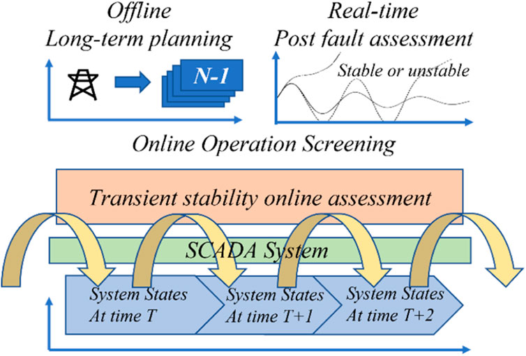
FIGURE 1. Power system transient stability assessment at different stages.

For the offline planning stage, when there is a new transmission line, a new generation unit needs to be added to the system, or other major renovations, the system transient stability needs to be re-assessed by all of the N-1 cases, under typical operating scenarios. Currently, most of the grid operators in US or China only perform N-1 tests with several typical scenarios, usually two scenarios for summer, and two scenarios for winter. These tests may cover some of the worst scenarios historically. However, due to the increasing penetration of renewable energy, these typical scenarios are no longer be able to provide reliable and not overly conservative operation references. Therefore, online assessments are needed. In addition, the time consumption of the offline assessments is not a primary concern, the TDS-based methods are usually implemented.

For the online operation stage, the operating conditions of the power system are constantly changing. The real and reactive power load and power generations from renewable energy resources are continuously fluctuating. The controllable resources and demand response resources are following the system needs. In real power systems, the states of the system can be acquired by the SCADA system with state estimations for every 5–15 min. And some of the resources which have fast response dynamics are re-scheduled or re-dispatched for every 15 min to 1 h. First, the system operating conditions are gained, and the power flow is calculated based on the new dispatch result. Then, a list of final security checks needs to be quickly conducted, including a set of N-1 tests of transient stability, before the dispatch signals are distributed. In the legacy grid, the operating conditions rarely have large, unpredictable variations within 15 min interval. With the development of renewable energy, the operating conditions are subject to larger fluctuations and the solar and wind forecasting usually provide potential ranges of active power output with certain confidence intervals. As a result, a faster, and more accurate online transient stability assessment capability is required to continue monitoring the system and guide the operations. A larger set of N-1 scenarios need to be assessed between every dispatch interval. These tests can provide much better references for the system operator, compared to offline analysis. The results of the online screening for transient stability are used for supporting the optimal dispatch and preventive controls for the online operations of power systems.

For the real-time post-fault stage, the transient rotor angle stability is determined mostly by the first swing, or several following swings (Kundur, 1994). This means the time frame is very short. The real-time assessment is combined with emergence control decisions and performed by comparing the fault and protection device action information with offline simulated scenarios. In addition, the use of phasor measurement unit (PMU) is limited by industry practice due the cyber security concerns.

In this work, we primarily focus on the transient stability assessment at the online operation stage, where lots of simulations and assessments need to be performed as soon as possible and as accurately as possible. Some of the features, proposed in this work, can be applied to the other two stages.

The power system transient stability assessment problem is a classification problem. After a disturbance, if the post-fault states trajectory is asymptotic stable and the final equilibrium point is a stable equilibrium point, then the system is stable. Otherwise, the system is unstable, or may fall into a limit cycle. In a real system, the operating condition at the post-fault stable equilibrium point should satisfy certain operating requirements. Actually, the transient stability is often referred to as the rotor angle stability of the system, which means that all the synchronous machines should remain synchronism. Based on the well-established engineering knowledge, the transient stability index (TSI) can be used to identify the stability of the system with the following equation (Tang et al., 1994),

where $∆{\delta }_{\mathit{max}}$ represents the maximum rotor angle differences between any two generators in the system. When $TSI$ is greater than 0, the system is stable. Otherwise, the system is unstable.

2.2 The proposed transient stability assessment framework

In this work, we proposed a comprehensive transient stability assessment framework for the online operation stage. The overall structure of the framework is shown in Figure 2. It consists of an offline preparation section, an online assessment section and an online updating section. The structure and workflow of the proposed framework are described in the following. The detailed formulations of multiple physics-informed neural networks (M-PINNs) and transfer learning with central moment discrepancies (CMD) is provided in section III and IV.

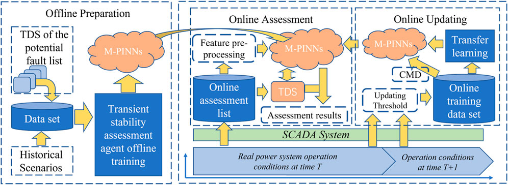
FIGURE 2. The proposed transient stability assessment framework.

2.2.1 Offline training section

To provide fast online transient stability assessment results, the proposed framework is a data-driven machine learning-based method. The M-PINNs need to be trained offline under well-established supervise learning procedures. The training data set is mainly generated by time-domain simulations of a potential fault list. To the best knowledge of the authors, this list usually contains a huge set of different faults, such as all of the N-1 faults and some important N-1-1 or N-2 fault scenarios. Notice that for a real power system, the “-1” refers to the loss of a component, not limited to line or generation losses. The component could also be a busbar at a substation or a tower carrying multiple lines. In addition, the simulations results of historically fault scenarios are also added to the data set. The TDS can provide the data input the M-PINNs needed, and the simulation results can be labeled by Equation 3 to supervise the training process. During the offline training the multi-fold cross-validation can be used to improve the data usage and the performance of the M-PINNs. After training with the fault scenarios under different operating conditions, a general transient stability assessment agent, M-PINNs, is produced for online operation.

2.2.2 Online assessment section

During the online operation of the power system, as stated above, the online assessment is needed to ensure the system’s safety. At each time-period, the system operating condition is collected by the SCADA system with state estimations. Then, the transient stability of a smaller list of potential fault scenarios should be investigated. This list is usually built based on the engineering knowledge of system operators. And various according to different operating conditions, such as power flow changes. Conventionally, the TDS is used, resulting in limited analyzation capability. In this work, the M-PINNs are used to work with TDS to generate reliable assessment results, the concept is shown as the following.

For TDS-based transient stability assessment, the per-fault, fault-on, and post-fault simulations are required. Usually, the post-fault simulations need to last for several seconds, which is time-consuming. For M-PINNs data driven-based transient stability assessment, only the first several hundred milliseconds (100–300 m) of the post-fault simulations are needed for the assessment. This means the M-PINNs method can drastically reduce the computation cost and time consumption for online assessment. Therefore, increasing the analyzation capability of the system to pre-screening more possible fault scenarios under changing operating conditions. If the assessment results from the M-PINNs surpass a pre-set confidence threshold, then, output the results. Otherwise, the full-length TDS is used to re-assess the low-confidence, high-risk scenarios. Therefore, the TDS and M-PINNs work together to provide reliable transient stability assessment results. In other words, the well-trained M-PINNs can solve the assessment tasks of easier potential fault scenarios in a timely manner, and find the hard ones for TDS to work with.

3 Features pre-processing and physics-informed neural networks

The section formulates the core part of the online transient stability assessment method, namely, the feature pre-processing module and the physics-informed neural networks. They will be running in parallel with the TDS during the online operation and provide quick stability assessment results.

3.1 Feature pre-processing module

The feature pre-processing module serves as the important interface between the TDS and the neural networks. It is crucial for improving the efficiency and accuracy of online assessments.

The TDS of power systems are performed with numerical methods, such as the Euler methods or Runge-Kutta methods. In this work, the TDS is developed based on the structure of the Power System Toolbox by Prof. J.H. Chow (Chow and Cheung, 1992). To further speed up the simulations, the Kron reduction is used, where all the non-active buses in the system are eliminated (Dörfler and Bullo, 2013), (Villegas Pico and Johnson, 2019). Generation buses, and the slack bus are kept in the simulation. In this reduction process, it also converts the power system from a sparse network to an all-to-all connection network. For any power system with a nodal admittance matrix,

where $N$ is the total number of buses. It is assumed that the non-generation nodes can be regarded as passive constant impedances during the transient period. Only the generation nodes have current injections. The $Y$ matrix can also be rearranged to the following form,

where $g$ represents the group of generation nodes, $p$ represents the group of passive nodes. The reduced network is,

where $Y_{red}$ is the reduced network admittance matrix. This means that during the TDS, only the state variables of the generation buses are available. The state variables of other internal buses, such as voltage magnitude or phase angle need additional calculations. In order to let the TDS and M-PINNs work together more efficiently, the M-PINNs will only take the states from generation buses. Details are provided in the next subsection.

The state parameters $\overline{X}$ of the generator buses are sampled per 0.01 s, from time $t_0$ to $\left(t_0+t_{end}\right)$. The sampled vector is $\overline{X}=\left[\begin{array}{cc}{x}_{t_0}& \begin{array}{cc}{x}_{t_1}& \begin{array}{cc}\begin{array}{ccc}\cdots & x_{t_m}& \cdots \end{array}& x_{t_{end}}\end{array}\end{array}\end{array}\right]$. And the $x_{t_m}$ is normalized by the following equation,

where $\mathit{max}$ and $\mathit{min}$ drives the maximum and minimum value of sampled vector of a state variable. $x_{t_m,nom}$ is the value after normalization. Notice that the state parameter $\overline{X}$ can be one of any generator parameters, like rotor angles, currents, voltages, etc. The parameters are only normalized with respect to the maximum and minimum values of its own class. For fast transient stability assessment, the sampling time window is usually few hundred milliseconds after the fault happened or fault cleared. Within this short time range, the state parameters will not have extremely large and small values due to the system inertia and control limits. Then, Equation 7 can be used to normalize the system parameters.

In computer science, information technology, and complex system community, the entropy is widely used for measuring the average level of useful “information”, extracting the “surprises”, or “changes” within a dataset. In previous works, an rule-based rapid stability assessment has been developed with the assistance of entropy measures (Kamwa et al., 2009). It should be noted that even though the time-series data from TDS contains all the information for stability assessment. The level of useful information in each state variable vector at different time-period is different. Some state variables contain much more detailed information about the fault and what happened thereafter, such as the voltage magnitude. Other state variables may preserve less information due to the limitations of simple and slow dynamics, such as the rotor speed. The information entropy equation is defined as the following,

where $X=\left[x_1,x_2,\dots ,x_i,\dots x_n\right]$ is the discretized vector of the state variable $\overline{X}$. $\left.{P(x}_1),P(x_2),\dots ,P(x_i),\dots P(x_n\right)$ are the probability of appearances. $H\left(X\right)$ is the information entropy value. Eq. 8 is used to extract the physical information from the TDS outputs. In case studies section, we will show that the M-PINNs can benefit from these inputs.

3.2 Multiple physics-informed neural networks

Neural network-based machine learning algorithms have strong fitting capabilities for high-order non-linear systems. By adopting the supervised learning training process, the neural networks can build the mappings between the input and labeled output, which is purely data-driven. Different from the previous works, we introduce the physics-informed concept to the transient stability assessment, the physics-informed neural networks (PINNs) not only can be driven by big data, but also informed by pre-established physics knowledge. In this way, the PINNs can be built, trained, and implemented more wisely and efficiently.

The structure of the PINN in this work is shown in Figure 3. The major components are input layer, hidden layer, pooling layer, activation function, fully connected layer, and output layer, as shown in Figure 3.

FIGURE 3. The structure of the PINN.

3.2.1 Input layer

The standard input layer for graph neural networks is used to link the input signals with the hidden layers in the middle. The number of input nodes equal to the number of buses in the target power system. As stated above, only the states from the generation buses are used. For other passive nodes, the information entropy of the system is used to fill in the blanks.

3.2.2 Hidden layer

The hidden layer is designed based on the structure of Chebyshev neural network, which is a branch of the spectral graph neural network.

Define a graph $G=\left(V,E,W\right)$, where $V$ and $E$ are the set of vertices and edges in $G$, $W$ is the adjacency matrix of $G$. Notice that if the power grid is considered as a graph, the vertices are the buses in power system; edges represent the transmission lines; $W$ preserve the topology information of the power grid; and $G$ is always a connected graph when the system is stable during the normal operation condition without any buses or lines tripped. Thus, we have

where $L$ is the normalized Laplace matrix, $I$ is the identity matrix, $D$ is the diagonal matrix with the following diagonal elements,

where $i$ and $j$ are indices of matrix $D$ and $W$. Define the eigenvectors of the normalized Laplace matrix $L$ as $\mathrm{U}=\left[{\mathrm{u}}_1,{\mathrm{u}}_2,...,{\mathrm{u}}_{\mathrm{n}}\right]$, and the matrix of eigenvalues as, $\mathrm{\Lambda }=\mathrm{d}\mathrm{i}\mathrm{a}\mathrm{g}\left({\lambda }_1,{\lambda }_2,...,{\lambda }_{\mathrm{n}}\right)$, where $L=U\Lambda U^T$. The Fourier transform on graph $G$ can be defined as,

where $\widehat{x}$ is the projection on the spectral domain through the orthogonal basis $U^T$ of the original input signal $x$.

Define the operator of spectral graph convolution as “${*}_G$”, and the operator of matrix dot product as “☉”. The spectral graph convolution between two signals $x$ and $y$ is derived as,

Let $U^{T}y={\left[{\theta }_0,{\theta }_1,...,{\theta }_{n-1}\right]}^T$, and define $g_{\theta }=diag\left(\left[{\theta }_0,{\theta }_1,...,{\theta }_{n-1}\right]\right)$ as the kernel function of the spectral graph convolution operation. The graph convolution on the spectral domain has the following expression

With Equations 9–13, the basic structure of PINN is established. The power systems topology and transmission line admittance matrix can be substitute or derived into the form of Equation 9, since the $Y_{bus}$ matrix has the similar formulation (Kundur, 1994). The physical law and physical model of the power system are embedded into the design of the neural networks. The PINNs in this work have the same number of vertices as the number of buses in the power grids.

In the above formulation, the information from all of the nodes in $V$ are needed for the calculations. This creates a huge computational burden for large power system with lots of buses. And it is also very inefficient, because the buses from far distances in power systems have marginal impacts on the local rotor dynamics. Buses/nodes nearby have the majority of the coupled impacts. Therefore, in this work, the Chebyshev polynomial expansions are used to approximate the graph convolution kernel $g_{\theta }$ (Michaël et al., 2016), (Tang et al., 2019), with the following expansions,

where $K$ is the number of polynomials, $\beta$ is a vector of coefficients. Substitute Equation 14 into Equation 13, the Chebyshev approximated spectral graph neural network is given by,

where the kernel is localized via convolutions with a Kronecker delta function (Hammond et al., 2011). Let $d_g$ represents shortest path distance between two vertices. $\forall d_g\left(i,j\right)>K$, ${\left(L^K\right)}_{i,j}=0$. This is a $K$-localized spectral filter with $K^{th}$-order polynomials of the Laplacian. In terms of the adjacency matrix $W$, it counts the number of edges between vertices $i$ and $j$. This process reduces the complexity of PINNs to the same level of conventional convolution neural network (CNN). With a good $K$ value, chosen based on the average distance between the nearest generation buses in a power grid, the inputs from generation buses can be collected and the computational burden is also well balanced.

Notice that even though the CNN is widely used in a lot of power system stability studies (Yan et al., 2021), (Yan et al., 2019), (Gupta et al., 2019), the convolution operation in CNN is not designed for the power engineering problems. It was originally designed for the computer vision and image recognition tasks with a critical assumption that the neighboring pixels in an image are correlated. Thus, the CNN algorithms convolute the information into the center pixel position from its neighbors. In power engineering problems, we can, for example, put the time-series voltage data of different buses into a 2-dimensional matrix and substitute it input the CNN. However, the voltage data does not share the same pre-assumption. The CNN-based methods were working simply because of the strong non-linear fitting capabilities of the CNN. The buses in a power grid are topologically correlated with transmission lines and power flows. Therefore, Equations 9–15 are used to build the linkage between vertices and edges in an undirected graph. And this graph is physically informed by the power grid network.

3.2.3 Pooling layer and activation function

Two different pooling layers are investigated in this work, namely, the local average pooling and the maximum value pooling over the kernel. And the maximum value pooling is chosen. The leak Relu activation function is used in the PINNs.

3.2.4 Fully connected layer and output layer

The fully connected layer in a deep network usually serves as a classifier. The hidden Chebyshev layers and pooling layers can build the mapping between the input and the internal feature space. And the fully connected layer can link the internal feature space with a labeled sample space. Lastly, the Softmax layer is used as the output layer to provide the final output. Instead of a single hard maximum output, the soft maximum provides the probability of each classification category, which can provide a valuable reference for the confidence of the classification results.

4 Online transient stability transfer learning with central moment discrepancy

The purpose of this online transfer learning is to further improve the assessment accuracy with real-time operating conditions acquired by the SCADA system. It used the offline trained model or the model from the previous time period as good baseline models, where a lot of general knowledge has been learned. Therefore, the online training workload is reduced and can focus on the cases and scenarios needed the most at the moment.

The proposed graph neural network-based PINN is firstly trained offline as the generalized model with numerals power system operating conditions and fault scenarios. It can provide fair transient stability assessment results in all cases.

It should be noted that the training process of neural networks can be considered as an optimization process, where the algorithm is trying to find the best-fit weights through the loss function and back propagation. If the faults scenarios and operating conditions of the training samples are evenly distributed in the offline training set. The algorithm will try to find the optimal parameters that achieves the minimum losses over the whole set. The idea is similar to the support vector machine model, which finds one best-fitting hyperplane to separate all the data samples by categories. The model is generalized in macroscopic but may lose accuracy in microscopic. Therefore, in this work, the transfer learning with central moment discrepancies is used to fine tuning the weights of the PINNs to provide better transient stability assessment results under online operating conditions.

4.1 The online transient stability transfer learning framework.

The proposed online transfer learning framework is shown in Figure 4.

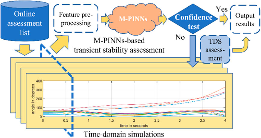
FIGURE 4. The structure of transfer learning for transient stability assessment.

The online transfer learning is initiated when the changes of the operating condition of the power system surpass the pre-set threshold. In this case, the changes are measured by using the standardized Euclidean distance,

where $n$ is number of dimensions of the measured operating conditions. $Y\left(y_1,y_2,\dots ,y_n\right)$ and $X\left(x_1,x_2,\dots ,x_n\right)$ are the neighboring operating conditions at time period $T$ and $T+1$. $s_i$ is the standard deviation of the $i$-th dimension. The standardized Euclidean distance over comes the problem of different scales between different dimensions. When $d>d_{threshold}$, the transfer learning will extract the current M-PINNs-based model from the online assessment framework and update it. Then the updated model will be used for the online assessment for the next time period.

4.2 The transfer learning with central moment discrepancy

The basic idea of transfer learning is to retrain the M-PINNs with training samples based on the current operating condition. Due to the time limitation, only a small number of training samples can be generated by TDS. In real-world operations, these small samples are selected based on the engineering knowledge. In addition, the training samples from previous similar operating conditions will be used to assist the transfer learning process. According to the transfer learning algorithm, the weights parameters of all the layers of M-PINNs are retrained with the following loss function (Zhu et al., 2021),

where $l\left(・\right)$ is the cross entropy loss function, $M$ is the number of the batch size, $z_i$ and $z_i^{\prime }$ are the output label and true lable of $i$-th sample. $\gamma$ is a scaler weight, $L_{regularizer}$ is a regularizer function to prevent the model from overfitting the small sample set by using the central moment discrepancy (CMD).

Consider that there is a mismatch between the distribution of the small transfer leanrning trainning set and the distribution of the potential fault cases set of a true system. To measure this distribution shift, many technics can be used, such as, the Kullback-Leibler divergence (KL), the maximum mean discrepancy (MMD) or CMD can be used. In this work, to achieve better online performance and faster speed, the CMD is adopted for the following reasons, 1) the KL-divergence approach only matches the first moment, which lacks of capability in higher order moments in the hidden activation space; 2) comparing with the MMD-based approach, which minimizes the distance between weighted sums of all moments with the Taylor expansion of the Gaussian kernel, the CMD does not require computationally expensive matrix computations (Zellinger et al., 2017). The $L_{regularizer}$ can be defined as,

where $E\left(Z_{train}\right)=1/M\sum z_{train,i}$ and $E\left(Z\right)=1/M\sum z_i$ are first order moment of the training set and the whole potential fault set. $c_k\left(Z_{train}\right)=E{\left(Z_{train}-E\left(Z_{train}\right)\right)}^k$ and $c_k\left(Z\right)=E{\left(Z-E\left(Z\right)\right)}^k$ are the $k$-th order moment. This regularizer term can be used to balance the fitting of the M-PINNs between the underfitting the potential fault scenarios under the current operating condition and the overfitting the small online transfer learning data set. In addition, the dropout mechanism is also used to prevent the overfitting.

5 Case study

5.1 Test system and data

In this paper, the proposed M-PINNs-based online transient stability assessment method is tested on a modified IEEE 16-machine 68-bus system, which is a benchmark equivalent model of the New England test system (NETS) and the New York power system (NYPS), as shown in Figure 5. The generators from G1 to G9 belong to NETS area, G10 to G13 belong to NYPS, and the neighboring areas are represented by G14, G15 and G16. To further include the renewable energy generations, the G10 and G11, G4 and G5 are replaced by lumped wind turbines with virtual synchronous machine (VSM) controls (Zhong, 2016), (Liu and Zhang, 2019). Notice that the VSM also has virtual generation parameters, which are equivalent to the conventional generators but subject to different dynamics according to primary energy sources. The sixth-order sub-transient model of the synchronous generators with a second-order exciter model, and a third-order PSS model has been implemented in the simulations (Liu et al., 2019). The parameters of the test system are from the Power System Toolbox (PST) (Chow and Cheung, 1992). All six types of faults from PST are considered, namely the three-phase fault, the line to ground fault, the line-to-line fault, line-to-line to ground fault, loss of line fault and loss of load at bus fault. The offline training data set is built where the fault types, fault locations and fault durations are randomly selected from six types of faults, on all buses and transmission lines, duration ranges from 3 cycles to 15 cycles with uniform distributions. The size of the offline training set is 10000 samples. The training set is generated by TDS with various simulation time steps, ranging from 1e-6 to 1e-3, according to the PST (Chow and Cheung, 1992).

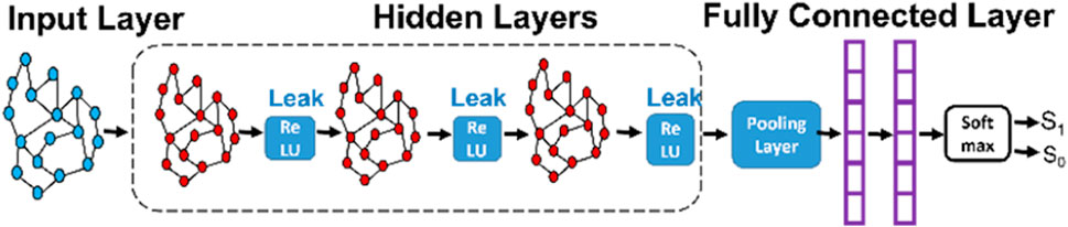
FIGURE 5. The single line diagram of the modified IEEE 16-machine 68-bus system.

5.2 Implementation and validation of the proposed framework

Using the test system and dataset, the proposed Chebyshev neural network-based M-PINNs models are firstly trained offline. The parameters in the hidden layers are trained with back propagation through the stochastic gradient descent method. In this work, the momentum mechanism is also used to further speed up the training process.

For inputs, the topology of the power system is adopted as the topology of the Chebyshev neural networks by Equation 9. The relative rotor angle, rotor speed, q-axis current and bus voltage magnitude of generators and VSMs are used as inputs for the network nodes of generation buses. The renewable generations can access the system through these VSMs. The information entropies of the above four measurements are used as the homogeneous inputs for all of the other nodes. The sampling rate for the inputs is 30 milliseconds, and the time window is 300 milliseconds from the moment of fault introduced. Notice that this time window is much shorter than some other works in literatures, since they used the fault clearing time as the starting point. This means that longer post-fault trajectories are accessible for the neural network model, which is easier. But the assessment results are produced slower than the proposed method in this work.

For the M-PINNs model setup, the concept of ensemble learning is adopted (Ren et al., 2015; Liu and Zhang, 2016; Liu et al., 2020). The M-PINNs model is consist of four PINNs. Each of them takes three out of four measurement inputs mentioned above, for example, one of the PINNs uses rotor speed, q-axis current, and bus voltage magnitude as inputs, no relative rotor angle. And the final decision is only made when at least three out of four PINNs agree with each other. This setup has several advantages. First, the model is more robust to random errors, because at least three independently trained must produce the same assessment results. Second, the model gained the capability of overcoming unexpected errors in one of the input states. Last but not least, when the assessment results are tied two by two amount four PINNs, this means that the results do not pass the confidence test. Thus, according to Figure 6, the samples will be sent back to the TDS for accurate assessment.

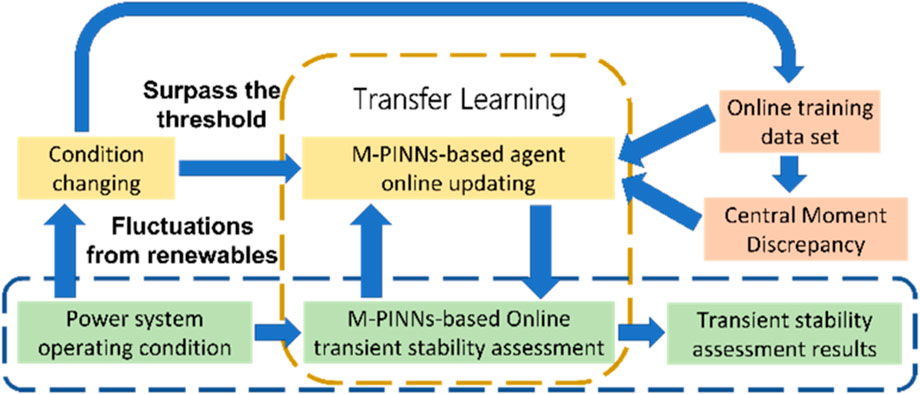
FIGURE 6. The coordination between TDS and M-PINNs.

The algorithm is implemented in TensorFlow and the power system model is built in MATLAB. The hyperparameters are shown in Table 1. The convergence of four PINNs of the proposed model during offline training is demonstrated by the accuracy curves in Figure 7.

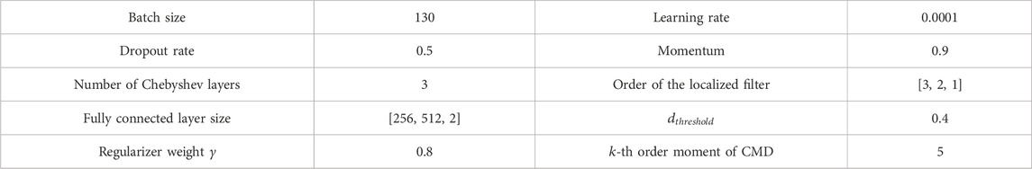
TABLE 1. The hyper parameters of M-PINNs model.

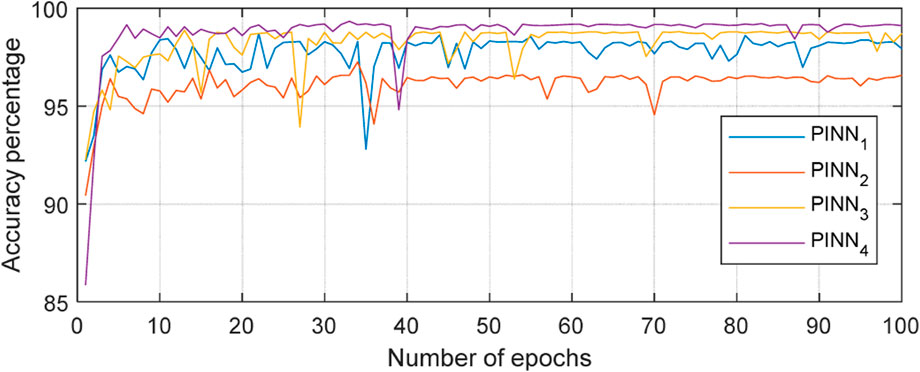
FIGURE 7. The accuracy curves of four PINNs during the training.

The accuracy of the proposed M-PINNs is compared with other machine learning-based algorithms in Table 2. For fairness, when the model has a tied result (2-2 even), the result from the PINN without rotor speed input is used as the final decision. The TDS is not used simply for a fair comparison. The “±” sign shows the variation ranges with 10 different random seeds. From the results, the proposed method has the best transient stability assessment accuracy. The overall accuracy of the proposed framework is 99.64%. Because the cases with tied results from M-PINNs are further verified with TDS.

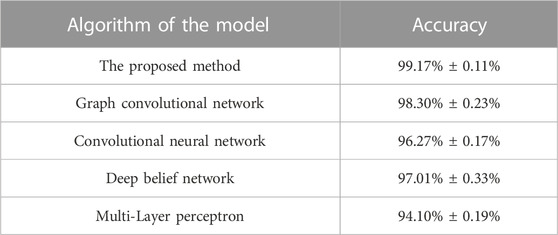
TABLE 2. The performance of Different models.

For the transfer learning performance, the results are shown in Table 3, including the five different operation scenarios and the results from a model without transfer learning, a model with transfer learning but no CMD, and the proposed model. It can be seen that the proposed model provides the best results again.

TABLE 3. The transfer learning performance of the proposed framework.

In addition, the t-distributed stochastic neighbor embedding (t-sne) algorithm is also implemented to show the classification process of the proposed PINN model in Figure 8.

FIGURE 8. The virtualization of the classification process of a PINN model.

T-sne is a non-linear dimension reduction method. It is commonly used in machine learning literatures to virtualize the deep neural network working process through neuron activations signal matrices. The subplot (a–f) in Figure 8 shows the activations of the input layer, the first Chebyshev graph convolution layer, the second Chebyshev graph convolution layer, the third Chebyshev graph convolution layer, the fully connected layer and the final Softmax layer. From the figure, we can see that the PINN model is effectively separated the stable cases, labeled as 1, and unstable cases, labeled as 0.

6 Conclusion

In this work, an online power system transient stability assessment framework is proposed with spectral graph convolution neural network-based M-PINNs and transfer learning with CMD technics. The designs of the framework are provided in detail. The proposed framework can be trained offline with physical information from the power grid, and work closely with time-domain simulations during the online assessment stage to provide fast and accurate results. The physical informed feature and CMD regularizer design provide the framework with strong capabilities to handle the system operation changes, due to the variations from the renewable generations.

For future works, under the practical scenarios with the penetration of power electronic devices interfaced resources, the emergency control actions are faster and may overlap with the time frame of assessment and protection actions. Therefore, a coordinated framework between the assessment-protection-control should be investigated as a valuable future research direction.

Data availability statement

The raw data supporting the conclusions of this article will be made available by the authors, without undue reservation.

Author contributions

ZL and XH wrote the manuscript; ZD built the simulation environment; ZL and PZ provided the conceptual idea; ZL performed all the experiments.

Funding

This work is supported by National Nature Science Foundation of China (52107068); Fundamental Research Funds for the Central Universities (2021JBM027).

Conflict of interest

The authors declare that the research was conducted in the absence of any commercial or financial relationships that could be construed as a potential conflict of interest.

Publisher’s note

All claims expressed in this article are solely those of the authors and do not necessarily represent those of their affiliated organizations, or those of the publisher, the editors and the reviewers. Any product that may be evaluated in this article, or claim that may be made by its manufacturer, is not guaranteed or endorsed by the publisher.

References

Bie, Z., Lin, Y., Li, G., and Li, F. (2017). Battling the extreme: A study on the power system resilience. Proc. IEEE 105 (7), 1253–1266. doi:10.1109/JPROC.2017.2679040
Che, Y., Cheng, C., Liu, Z., and Zhang, Z. J. (2020). Fast basin stability estimation for dynamic systems under large perturbations with sequential support vector machine. Phys. D. Nonlinear Phenom. 405, 132381. doi:10.1016/j.physd.2020.132381
Chiang, H.-D. (2011). Direct Methods for Stability Analysis of Electric Power Systems: Theoretical Foundation, BCU Methodologies, and Applications. John Wiley & Sons. Hoboken, NJ, USA
Chiang, H.-D., and Thorp, J. S. (1989). The closest unstable equilibrium point method for power system dynamic security assessment. IEEE Trans. Circuits Syst. 36 (9), 1187–1200. doi:10.1109/31.34664
Chiang, H., Wu, F. F., and Varaiya, P. P. (1994). A BCU method for direct analysis of power system transient stability. IEEE Trans. Power Syst. 9 (3), 1194–1208. doi:10.1109/59.336079
Chow, J. H., and Cheung, K. W. (1992). A toolbox for power system dynamics and control engineering education and research. IEEE Trans. Power Syst. 7 (4), 1559–1564. doi:10.1109/59.207380
Dörfler, F., and Bullo, F. (2013). Kron reduction of graphs with applications to electrical networks. IEEE Trans. Circuits Syst. I Regul. Pap. 60 (1), 150–163. doi:10.1109/TCSI.2012.2215780
Gupta, A., Gurrala, G., and Sastry, P. S. (2019). An online power system stability monitoring system using convolutional neural networks. IEEE Trans. Power Syst. 34 (2), 864–872. doi:10.1109/TPWRS.2018.2872505
Hammond, D. K., Vandergheynst, P., and Gribonval, R. (2011). Wavelets on graphs via spectral graph theory. Appl. Comput. Harmon. Anal. 30 (2), 129–150. doi:10.1016/j.acha.2010.04.005
Huang, J., Guan, L., Su, Y., Yao, H., Guo, M., and Zhong, Z. (2020). Recurrent graph convolutional network-based multi-task transient stability assessment framework in power system. IEEE Access 8, 93283–93296. doi:10.1109/ACCESS.2020.2991263
Kamwa, I., Samantaray, S. R., and Joós, G. (2009). Development of rule-based classifiers for rapid stability assessment of wide-area post-disturbance records. IEEE Trans. Power Syst. 24 (1), 258–270. doi:10.1109/TPWRS.2008.2009430
Karniadakis, G. E., Kevrekidis, I. G., Lu, L., Perdikaris, P., Wang, S., and Yang, L. (2021). Physics-informed machine learning. Nat. Rev. Phys. 3 (6), 422–440. doi:10.1038/s42254-021-00314-5
Liu, X., Zhang, X., Chen, L., Xu, F., and Feng, C. (2020). Data-driven transient stability assessment model considering network topology changes via mahalanobis kernel regression and ensemble learning. J. Mod. Power Syst. Clean. Energy 8 (6), 1080–1091. doi:10.35833/MPCE.2020.000341
Liu, Z., He, X., Ding, Z., and Zhang, Z. (2019). A basin stability based metric for ranking the transient stability of generators. IEEE Trans. Ind. Inf. 15 (3), 1450–1459. doi:10.1109/TII.2018.2846700
Liu, Z., and Zhang, Z. (2019). Probabilistic-based transient stability assessment of power systems with virtual synchronous machines. IEEE Int. Symposium Industrial Electron. 2019. doi:10.1109/ISIE.2019.8781299
Liu, Z., and Zhang, Z. “Solar forecasting by K-Nearest Neighbors method with weather classification and physical model,” in Proceedings of the NAPS 2016 - 48th North Am. Power Symp. Proc.,2016 Denver, CO, USA, September 2016. doi:10.1109/NAPS.2016.7747859
Michaël, D., Xavier, B., and Pierre, V. (2016). “Convolutional neural networks on graphs with fast localized spectral filtering michaël,” in Proceedings of the 30th Conference Neural Information Processing Systems (NIPS), Barcelona, Spain, December 2016, 395–398.
Raissi, M., Perdikaris, P., and Karniadakis, G. E. (2017). Physics informed deep learning (Part II): Data-driven discovery of nonlinear partial differential equations. Available: http://arxiv.org/abs/1711.10566.
Raissi, M., Perdikaris, P., and Karniadakis, G. E. (2019). Physics-informed neural networks: A deep learning framework for solving forward and inverse problems involving nonlinear partial differential equations. J. Comput. Phys. 378, 686–707. doi:10.1016/j.jcp.2018.10.045
Ren, Y., Suganthan, P. N., and Srikanth, N. (2015). Ensemble methods for wind and solar power forecasting—a state-of-the-art review. Renew. Sustain. Energy Rev. 50, 82–91. doi:10.1016/j.rser.2015.04.081
Tang, C. K., Graham, C. E., El-Kady, M., and Alden, R. T. H. (1994). Transient stability index from conventional time domain simulation. IEEE Trans. Power Syst. 9 (3), 1524–1530. doi:10.1109/59.336108
Tang, S., Li, B., and Yu, H. (2019). ChebNet: Efficient and stable constructions of deep neural networks with rectified power units using Chebyshev approximations. [Online]. Available:.http://arxiv.org/abs/1911.05467
Villegas Pico, H. N., and Johnson, B. B. (2019). Transient stability assessment of multi-machine multi-converter power systems. IEEE Trans. Power Syst. 8950 (), 3504–3514. doi:10.1109/tpwrs.2019.2898182
Yan, R., Geng, G., Jiang, Q., and Li, Y. (2019). Fast transient stability batch assessment using cascaded convolutional neural networks. Fast Transient Stab. Batch Assess. Using Cascaded Convolutional Neural Netw. 34 (4), 2802–2813. doi:10.1109/tpwrs.2019.2895592
Yan, R., Wang, Z., Yuan, Y., Geng, G., and Jiang, Q. (2021). Information entropy based prioritization strategy for data-driven transient stability batch assessment. CSEE J. Power Energy Syst. 7 (3), 443–455. doi:10.17775/CSEEJPES.2020.04500
Zellinger, W., Lughofer, E., Saminger-Platz, S., Grubinger, T., and Natschläger, T. (2017). “Central moment discrepancy (CMD) for domain-invariant representation learning,” in Proceedings of the 5th International Conference on Learning Representations, ICLR 2017, France, Europe , May 2017, 1–13.
Zhong, Q. C. (2016). Virtual synchronous machines: A unified interface for grid integration. IEEE Power Electron. Mag. 3 (4), 18–27. doi:10.1109/MPEL.2016.2614906
Keywords: transient stability assessment, graph neural network, physics-informed neural network, central moment discrepancy, deep learning
Citation: Liu Z, Ding Z, Huang X and Zhang P (2023) An online power system transient stability assessment method based on graph neural network and central moment discrepancy. Front. Energy Res. 11:1082534. doi: 10.3389/fenrg.2023.1082534
Received: 28 October 2022; Accepted: 06 January 2023;
Published: 17 February 2023.
Edited by:
Jun Liu, Xi’an Jiaotong University, ChinaCopyright © 2023 Liu, Ding, Huang and Zhang. This is an open-access article distributed under the terms of the Creative Commons Attribution License (CC BY). The use, distribution or reproduction in other forums is permitted, provided the original author(s) and the copyright owner(s) are credited and that the original publication in this journal is cited, in accordance with accepted academic practice. No use, distribution or reproduction is permitted which does not comply with these terms.
*Correspondence: Zhao Liu, liuzhao1@bjtu.edu.cn; Xiaoge Huang, xhuang98@binghamton.edu