Optimal Power Flow of Renewable-Integrated Power Systems Using a Gaussian Bare-Bones Levy-Flight Firefly Algorithm

1 Introduction

Since its start approximately half a century ago, optimal power flow (OPF) has remained a popular topic among power system researchers. The primary goal of OPF is to reduce generating costs by adjusting control variables such as produced actual power and network generator bus voltages to their optimal values. System limitations in generator capabilities, power flow equations, line thermal limit, and bus voltage limits must be met while optimizing generation costs. The ideal operational status of the system is represented by the programmed power of the generator, the complicated power flow in the lines, and the bus voltage vector established throughout the optimization procedure. The typical OPF problem involves thermal power producers using fossil fuels to produce electricity (Niknam et al., 2013). With the growing use of solar and wind-based distributed generations in the electricity grids, a study of OPF is required to account for the uncertainties associated with these renewable energy sources.

Researchers from all around the world have researched OPF using simply thermal power generators. A recent study used the moth swarm algorithm (MSA) (Mohamed et al., 2017) to demonstrate the algorithm’s efficiency in terms of rapid running time and rapid convergence for various OPF objectives for several bus systems. Lévy mutation-enhanced teaching–learning-based optimization (TLBO) (LTLBO) (Ghasemi et al., 2015a), grey wolf optimizer (GWO) (El-Fergany and Hasanien, 2015), a unique method to multi-objective OPF using a new hybrid optimizer that considers generator limitations and multi-fuel type (Narimani et al., 2013), and a revised bacteria foraging (Panda et al., 2017). In (Bouchekara et al., 2016), an improved colliding bodies optimization (ICBO) method is presented. Increasing the number of colliding bodies raises the algorithm’s findings, which is a benefit for addressing the OPF problem. Using the backtracking search algorithm (BSA) technique, authors (Chaib et al., 2016) have calculated OPF with more complicated objectives of multi-fuel choices and incorporated the valve-point effect. A typical approach for optimizing group searches has been enhanced using adaptive group search optimization (AGSO) (Daryan et al., 2016). In (Khorsandi et al., 2013; Rezaei Adaryani and Karami, 2013; Ayan et al., 2015; He et al., 2015), the various kinds of artificial bee colony (ABC) algorithm such as basic ABC, improved ABC (IABC), a chaotic ABC (CABC), and a modified ABC (MABC) for solving OPF problems have been implemented and compared. Also, to deal with the OPF problems, an enhanced multi-objective Quasi-reflected Jellyfish search algorithm (MOQRJFS) (Shaheen et al., 2021), MOELA (multiobjective electromagnetism-like algorithm) (Jeddi, Einaddin and Kazemzadeh, 2016), an improved adaptive differential evolution (DE) (Li et al., 2020), a new version of salp swarm algorithm (SSA) (Kamel, Ebeed and Jurado, 2021), a multi-regional OPF considering load and generation variability using marine predators algorithm (MPA) (Swief et al., 2021), BAT search algorithm (Venkateswara Rao and Nagesh Kumar, 2015), a multi-objective evolutionary algorithm with constraint handling technique based on non-dominated sorting (Li et al., 2022), an enhanced MSA (EMSA) based on quasi-opposition-based learning (Bentouati et al., 2021), delicate flower pollination algorithm (DFPA) (Dhivya et al., 2021), levy spiral flight equilibrium optimizer (LSFEO) for OPF incorporating center node unified power flow controller (CUPFC) (Mostafa et al., 2021), teaching-learning-studying-based optimizer (TLSBO) (Akbari, 2022), boundary assigned animal migration optimization (BA-AMO) (Dash et al., 2022), an adaptive Quasi-oppositional differential migrated biogeography-based optimization (AQODMBBO) (Pravina et al., 2021), a new variable neighborhood descent (VND) method to solve OPF for large-scale networks (Home-Ortiz et al., 2021), a sine-cosine mutation operator and a modified Jaya (SCM-MJ) (Gupta et al., 2021), tunicate swarm algorithm (TSA) (El-Sehiemy, 2022), chaos embedded particle swarm optimization (CEPSO) (Daghan, Gencoglu and Özdemır, 2021), sparrow search algorithm (SSA) (Jebaraj and Sakthivel, 2022), chaotic Bonobo optimizer (CBO) to the OPF problem with stochastic renewable energy sources (RESs) (Hassan et al., 2022), and SSO (social spider optimization) (Nguyen, 2019) have been developed. Differential search algorithm (DSA) (Abaci and Yamacli, 2016) and a novel parallel genetic algorithm (PGA), i.e., EPGA (Mahdad et al., 2010), are a newly developed technique that applies the most advanced evolutionary algorithm (EA) to a few established OPF goals for thermal-integrated power systems.

While the above research works solely handle standard generator models, a system including generators that rely on both wind and thermal power has lately been investigated in a few works of literature in the search for the lowest generating cost. The literature (Zhou et al., 2011) has presented a dynamic economic dispatch (DED) model in the presence of large-scale wind generation while considering risk reserve restrictions. The authors (Mishra et al., 2011) have used the DFIG wind turbine model to solve the same problem. A modified hybrid, PSOGSA, of PSO and gravitational search algorithm (GSA) with chaotic maps methodology considering the uncertainties of solar radiation and wind speed using a stochastic model has been introduced (Biswas et al., 2017), a sine-cosine algorithm for OPF-based hydro-thermal wind scheduling in hybrid power systems have been presented in (Dasgupta et al., 2020). Multi-objective dynamic OPF (MODOPF) of wind integrated power systems with demand response has been investigated (Ma et al., 2019). Pumped hydro storage has been discussed in (Kusakana, 2016) as a possible alternative to battery storing for a comparable freestanding hybrid system composed of solar photovoltaic panels, wind turbines, and a diesel generator.

Several papers have explored how wind and solar photovoltaic (PV) energy resources can be integrated into the grid. Reference (Tazvinga et al., 2015) has covered the optimal planning for an isolated hybrid power system comprising a PV system, a diesel generator, and battery storage. Symbiotic organisms search (SOS) and moth swarm algorithm (MSA) have been used to solve the alternating current OPF (ACOPF) issue for thermal, wind, solar, and tidal energy systems (Duman et al., 2019; Elattar, 2019; Duman et al., 2021). In (Shi et al., 2011) the, authors have presented a methodology for estimating the cost of wind-based generation power. The issue of generator scheduling for economic load dispatch is particularly prevalent in systems with wind-based and thermal-based generation units. OPF in wind-thermal power systems has been solved using genetic TLBO (G-TLBO) (Güçyetmez and Çam, 2016). Reference (Dubey et al., 2015) has included the generator’s emission and valve-point loading impact in the DED optimization problem. A simulation tool for wind generation in OPF dispatching has been developed (Jabr and Pal, 2008). In (Roy and Jadhav, 2015), the Gbest-directed ABC(GABC) has been used to improve the optimal solutions to the OPF problems compared to other literature.

To investigate the effects of reactive power generations on the optimum results of OPF problems, a model incorporating static synchronous compensator (STATCOM) has been introduced in (Panda and Tripathy, 2015), and the OPF problem has been solved utilizing ant colony optimization (ACO). In (Panda and Tripathy, 2014), a modified bacterium foraging algorithm (MBFA) has been suggested, and a doubly fed induction generator (DFIG) model has been integrated into the OPF framework to describe the capacity of reactive power production.

The primary impediment to grid integration of wind and solar photovoltaic energy is their intermittent nature. Typically, wind farms and solar photovoltaic (PV) farms are funded by individual operators. The independent system operator (ISO) enters an arrangement with these private operators to purchase scheduled power. However, because the output of these renewable sources is unpredictable, power productivity might occasionally exceed the scheduled power, resulting in an underestimate of the existing quantity. ISO is responsible for the penalty cost associated with unused excess electricity. On the other hand, underestimation occurs when generated power is below scheduled power (Biswas et al., 2017). To balance power demand, ISO must maintain a spinning reserve that increases the system’s running costs.

To address the uncertainties of renewable generations, the Weibull probability density function (PDF) models the wind distribution in this work, whereas the lognormal probability density function models solar irradiation. The IEEE-30 bus system (Biswas et al., 2017) has been updated to support wind turbines and solar photovoltaic (PV) systems with reactive power capability. Beyond the producing cost of thermal power units, the objective function presented in this study includes the reserve, direct, and penalty costs of renewable energy sources. The total generation costs are considered the fitness function, and the effect of varying the penalty and reserve costs on optimum scheduling is examined. In terms of emissions, thermal generators powered by fossil fuels produce hazardous gases into the environment, whereas renewable sources do not. Carbon taxes (Yao et al., 2012) are levied in certain nations in proportion to greenhouse gas emissions. In studied cases, the amount of carbon tax is linked to the goal function to examine the influence on generator scheduling.

To solve such a complicated and nonconvex optimization problem, in this work, a Gaussian bare-bones Lévy-flight firefly algorithm (GBLFA) and its modified version, i.e., MGBLFA are introduced. Yang developed the firefly algorithm (FA) to expedite exploration and exploitation, motivated by the flashing patterns and behaviors of fireflies (Yang, 2010a). Many works have employed this algorithm in optimization problems. Reference (Jain and Katarya, 2019) has employed the FA to ascertain the opinion leader in online social networks. In (Sánchez et al., 2017), FA has been used in modular granular neural networks to provide parameter estimation for expert systems utilizing ear and face recognition (Yang et al., 2012), an FA technique for addressing the economic dispatch problem in the context of real power system management has been suggested, in (Wang, 2012), the FA to unmanned combat air vehicle path planning has been applied, in (Langari et al., 2020), fuzzy clustering in conjunction with FA to secure the anonymized database and reduce information loss has been used, and in (Kavousi-Fard et al., 2014), the FA to determine the optimal value for accurate short load forecasting in support vector regression has been employed. However, an efficient version of FA has not been introduced for optimizing the various kinds of OPF problems in the previous works. In addition, other reviewed optimization algorithms still need some improvements in terms of robustness, avoiding local optimal solutions and finding better solutions, and improving convergence characteristics. Hence, this paper tries to fulfill such gaps and improves the quality of optimal solutions by improving the performance of FA via strategically utilizing Lévy-flight, bare-bone, and Gaussian sampling.

This paper is structured as follows. Section 2 introduces the OPF problem formulation. The basic firefly algorithm (FA), the levy-flight FA (LFA), and our GBLFA and its modified version (MGBLFA) are all detailed in Section 3. Then, in Section 4, simulation results on ten OPF problems are presented. Finally, some concluding remarks are given in Section 5.

2 Problem Formulation

The OPF problem is a nonconvex and non-linear optimization problem in which specific objectives of power systems are minimized/maximized subject to numerous inequality and equality constraints. In a general form, an OPF problem can be briefly expressed as follows (Ghasemi et al., 2015b; Mohamed et al., 2017):

Where J(x, u) indicates the desired objective function(s) to be maximized/minimized, which may include economic, environmental, and technical goals, equality and inequality constraints are defined by g(x, u) and h(x, u), respectively. x indicates the power system-dependent variables, and u defines the control/independent variables.

In this paper, the system-dependent variables include P_G1, V_L, Q_G, and S_l, which indicate the real power generation at the substation (slack) bus, load buses’ voltage magnitude, and reactive output power generated from generators, and lines’ apparent power flow. The total number of load buses, generator buses, and transmission lines are respectively indicated by NPQ, NG, and NTL. The independent control variables include P_G, V_G, Q_C, and T, which indicate the generators’ active power, the voltage magnitude at generator buses, the transformer’s tap position, and the reactive power generated from the shunt VAR compensators. The total number of tap positions and compensator units are defined by NT and NC, respectively.

2.1 Constraints

Both inequality and equality constraints should be addressed in the OPF problem. The limitations on the power balance are regarded as a restriction on equality. The operational limitations of the power systems are regarded as limiting inequalities.

2.1.1 Equality Constraints

The active and reactive power balance equalities at each load bus are given in Eq. 4, Eq. 5 respectively.

The active and reactive power demands at each load node are indicated by P_D and Q_D, respectively_. The conductance and susceptance of the branch between the adjacent load buses i and j are defined by B_ij and G_ij, respectively. Also, the total number of load nodes is indicated by NB. These equality constraints should be satisfied during the process of load flow which ensures that the solution found is optimal.

2.1.2 Inequality Constraints

The OPF inequality constraints indicate the operational limits of the power system, including limits on the generation buses, transformer tap operation limit, shunt VAR capacity limit, and security limits.

2.1.2.1 Generation Limits

in the steady-state operation mode, the active and reactive output power generation of generators, as well as the voltage magnitude at generator bus i ($i=1,\dots , NG$), should be limited between their lower and upper bounds as follows:

where for ith generator, $P_{Gi}^{\min }$ and $P_{Gi}^{\max }$ indicate the maximum and minimum limits of the active power output, respectively. $Q_{Gi}^{\min }$ and $Q_{Gi}^{\max }$ specify the lower and upper bounds of the reactive power output, respectively. $V_{Gi}^{\min }$ and $V_{Gi}^{\max }$ indicate the allowable voltage limitations.

2.1.2.2 Transformer Restrictions

Transformer receptacle adjustments should be limited by their higher and lower limits as follows:

In Eq. 9, the $T_i^{\min }$ and $T_i^{\max }$ are the lower and upper bounds of the tap position at the ith transformer.

2.1.2.3 Shunt VAR Trim Constraints

The VAR bypass margins are restricted by their limitations as follows:

where $Q_{Ci}^{\max }$ and $Q_{Ci}^{\min }$ indicate the allowable VAR injection for compensating unit i.

2.1.2.4 Security Limitations

The restrictions of charging buses should be controlled in the following terms: voltage levels and transmission line loading:

In Eq. 12, $S_{li}$ and $S_{li}^{max}$ indicate the seeming force and its upper boundary by the ith transmission line.

2.2 Constraints Handling

The inequity limitations of the dependent variables are considered in the extended objective function to maintain the control variables within their permissible limits. These force the optimization algorithm to find feasible solutions by satisfying the inequality constraints. The penalty function is defined according to a quadratic term as follows (Ghasemi et al., 2015a; Mohamed et al., 2017):

Where λ_P, λ_Q, λ_V, and λ_S are the penalty factors associated with the constraints’ violation in Eq. 6, Eq. 7, Eq. 11, and Eq. 13, respectively. Assuming z as a variable, z^lim is used to indicate each constraint violation as follows:

According to (Eq. 13) and (Eq. 15), no ppenalty is considered if a constraint satisfied. Suppose the value of the variable exceeds the upper/lower limit. In that case, the square of this violation is considered in the penalty function.

2.3 OPF Considering Stochastic Wind and Solar Power

In general, one or more objective functions are used to represent the OPF problem for a power network system that incorporates renewable energy sources. Renewable energy networks are linked to an IEEE 30-bus network system (Biswas et al., 2017) in several geographical situations in this article. Wind and solar energy are important contributors to OPF issues (Zargar et al., 2020; Farsani and Zare, 2021). To incorporate alternative fuels into the OPF issue, the power profiles of renewable energy sources are employed as a negative load (Saeidi et al., 2019). Wind and photovoltaic power generators are employed beforehand to provide loads, followed by thermal generators to meet remaining loads and network losses (Biswas et al., 2017).

2.3.1 Wind Power Modeling

A potential wind energy profile had been anticipated to create an effective optimization model for addressing OPF issues. The predictors in this article are generated using a Weibull probability distribution function. Prior to establishing the optimal solution technique, the wind energy estimating work can be completed autonomously. Generally, wind energy generation models are constructed using wind speed data (Panda and Tripathy, 2014; Panda and Tripathy, 2015; Roy and Jadhav, 2015). The wind speed is reported and probabilistically simulated in this section using the Weibull probability distribution function. The wind speed, f_v(v), is denoted by the symbol (Biswas et al., 2017):

where the wind speed $f_{\nu }\left(\nu \right)$ is described by the Weibull function based on the dimensionless shape factor (K) of the Weibull distribution and scale factor (c). As seen in Eq. 17, the mean of the Weibull distribution M_wbl is highly reliant on the gamma function Γ(x), as defined in Eq. 18 (Biswas et al., 2017).

Wind turbines can generally convert the wind’s kinetic energy to electrical energy. Eq. 19 presents the real output power of a wind turbine, P_w(v), as a function of wind speed (Biswas et al., 2017).

Where P_wr is the wind turbine’s rated power, v_in denotes the wind turbine’s cut-in wind speed, v_out denotes the wind turbine’s cut-out wind speed, and v_r denotes the wind turbine’s rated wind speed. As mentioned, the optimization technique in this work incorporates a random process using Weibull probability distribution simulation. This simulation gives the wind energy generation uncertainty. Moreover, the impact of wind turbine positioning and variations in wind speed profile on the optimum power flow formulation has not been studied previously. To estimate the cost of wind generation units in this article and to reduce the total cost of power generation, the expense of wind power generation units must be identified. The total cost of a wind power unit is represented based on wind speed and power output for considering wind uncertainties in the optimization problem. The direct, reserve, and penalty costs are computed in (USD/h) using Eq. 20, Eq. 21, Eq. 22. The overall cost of wind energy generation is (USD/h), $C_W^T$ is defined by Eq. 23 (Panda and Tripathy, 2014; Panda and Tripathy, 2015; Roy and Jadhav, 2015; Biswas et al., 2017). It consists of three major components: the direct cost of the wind turbine, the reserve or overestimation cost, and the penalty cost.

Supply companies for wind energy frequently provide anticipated power generation profiles. The network operator uses wind energy predictions to develop an operation plan for all producing units required to meet demand. If the real wind energy output is lower than expected, the extra cost is added to compensate. If actual wind energy output exceeds expectations, a penalty is applied (underestimation). As a result, an accurate calculation of the wind power profile is important. The actual material, reserve cost, and penalty cost are computed in USD/h, described in Section 4.

2.3.2 Solar Power Modeling

Sun energy is stochastic and volatile due to meteorological factors, including clouds and solar irradiation. As a result, the power output of solar systems is determined by the variable of Sun irradiance (G). The Sun irradiation (G) is given and probabilistically represented in this section using the lognormal probability distribution function, in which the probability function, denoted by f_G(G), is expressed as follows (Biswas et al., 2017):

The Solar System’s objective is to convert solar energy to electrical energy. Eq. 25 defines the output power of the Solar System, P_s(G), as a function based on the solar irradiance calculation in (24) (Reddy et al., 2014a).

Like wind power units, total solar energy generating costs are estimated in three terms: direct solar generation costs, reserve or excess estimates and penalty costs to reduce the effect of insecurity on estimating costs in solar energy profiles. In Eq. 26, Eq. 27, Eq. 28, in each case, the straight, reserve and penalty costs in USD/h are computed (Biswas et al., 2017). The equation describes the overall costs of solar production in (USD/h) CTS (29).

3 Proposed Optimization Algorithm

3.1 FA

FA is a metaheuristic algorithm that employs three main rules to construct the optimization algorithm based on the flashing behavior of fireflies and the biological communication phenomenon as follows (Yang, 2010b).

3.1.1 Rule 1

All fireflies come in unisex, which means that any firefly will be drawn to another irrespective of gender.

3.1.2 Rule 2

The attraction is related to the fireflies’ brightness, meaning that two flashing fireflies will gravitate towards the brightest. If no firefly is as bright as a specific fly, it will move randomly.

3.1.3 Rule 3

The brilliance of a firefly is impacted or decided by the objective function’s landscape. The brightness might easily be proportionate to the objective function value in a maximizing issue. Other types of brightness can be specified similarly to how the fitness function is established in genetic algorithms or the bacterial foraging algorithm (BFA) is developed (Yang, 2010a).

In FA, it is assumed that every firefly’s attraction directly depends on its brightness which depends on the fitness function. Firefly will be pulled toward a lighter firefly. Moreover, the brightness decreases as a function of the Cartesian distance (r) as a function of the reverse square law, as follows:

Additionally, the light intensity I through a given material with a constant light absorption coefficient $\gamma$ changes with the distance r from the source light as follows:

I₀ is the source of light intensity.

Since the attraction of a firefly is related to the luminous intensity observed by nearby fireflies, the attractiveness $\beta$ of firefly can be expressed as follows:

Here, parameter ${\beta }_0$ is the attractiveness at r = 0 and generally is set equal to 1.

For a given set of feasible solutions (fireflies), the light intensities are calculated, and every firefly will move towards the firefly with a lighter intensity. The best solution, i.e., the brightest firefly, will randomly move around its neighborhood to perform a local search. For the two fireflies i and j, where the light intensity j is higher than that of i, the location update of firefly i can be obtained as follows:

Where $\alpha$ and $\epsilon$ are randomization parameters and random vectors from a uniform distribution between 0 and 1, note that the last term in Eq. 33 is used for the brightest firefly and others, it can be omitted.

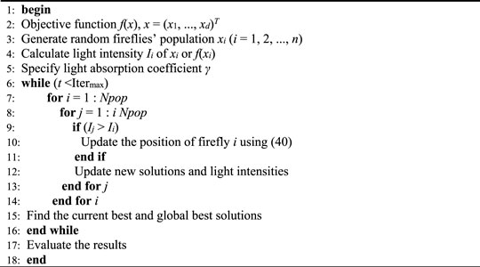
3.2 LFA

The randomization characteristic of conventional FA has been improved by (Yang, 2010b) by utilizing Lévy flights in the last term of Eq. 33 as follows:

where the entry multiplication is defined by $\oplus$, and $sign\left[rand-1/2\right]$ is utilized to provide random direction. The random step size is defined here using the Lévy distribution function with infinite variance and means as follows:

In this paper, ${\beta }_0$, $\gamma$, and $\lambda$ are set equal to 1, 1, and 1.5, respectively. Also, $\alpha$ is selected randomly between 0 and 1. The pseudo-code of the LFA is summarized in Algorithm 1.

Algorithm 1. LFA (Yang, 2010a)

3.3 Bare-Bones PSO (BBPSO)

PSO is a swarm intelligence-based method inspired by bird flocking and fish schooling behavior (Kennedy and Eberhart, 1995) that begins during exploration and continues until exploitation. This can be advantageous while searching for a variety of evolutionary optimization techniques. This study proposes a novel and strong LFA algorithm based on this concept, i.e., GBLFA. In the proposed algorithm, the Gaussian mutation approach of LFA is specified as follows:

Each particle is drawn to this method by its personal best position (P_best), and the global best position (G_best) discovered thus far. According to several theoretical studies (Vandenbergh and Engelbrecht, 2006), the individual particles gather around the weighted average of P_best and G_best:

Here, c₁ and c₂ are two learning factors in the PSO algorithm.

A bare-bones PSO (BBPSO) method based on the convergence characteristic of PSO has been developed (Kennedy, 2003). The velocity term is eliminated in this revised version of the PSO algorithm, and the location is adjusted as follows:

In which rand_j(0, 1) is a haphazard amount between 0 and 1 for the jth dimension, and N represents a Gaussian distribution with mean $(G_{best}+P_{bes{t}_{i,j,G}})/2$ and standard deviation | $G_{best}-P_{bes{t}_{i,j,G}}$ |. There is a 50% probability that the alternate method will focus on the prior best locations.

3.4 Bare-Bones DE (BBDE)

In (Omran et al., 2009), a novel and efficient version of DE using improved BBPSO and DE algorithms has been developed. In this algorithm, a new position is updated as follows:

where CR ∈ (0, 1) is the crossover factor. i₁, i₂, and i₃ are three indices chosen from the set {1, 2, . . ., Np} with i₁≠i₂ ≠ i. r_2,j and r_2,j are random numbers between 0 and 1 for the jth dimension.

3.5 Gaussian Bare-Bones LFA (GBLFA)

Gaussian sampling, as demonstrated by the exploration behaviors of BBPSO and BBDE, is a fine-tuning technique.

N represents a Gaussian distribution with mean $(x_j+x_i)/2$ and standard deviation $|x_j-x_i|$.

3.6 Modified Gaussian Bare-Bones LFA (MGBLFA)

Gaussian sampling may result in a slow convergence speed for the GBLFA algorithm. The hybrid version of GBLFA and DE/current-to-best/1 is discussed in this article. In (Das and Suganthan, 2010) are utilized to balance global searching and convergence speed. Thus, in this updated method, the search phase is adjusted as follows:

Additionally, a hybrid variant of this search phrase is utilized in conjunction with the strong DE/current-to-best/1 to improve the strength of both local seeking and the search phase. This minor adjustment, which included a diverse population, significantly improved the optimal solutions of MGBLFA.

This modified version of GBLFA is called MGBLFA in this article. The MGBLFA pseudo-code is summarized in Algorithm 2 as follows:

Algorithm 2. MGBLFA Algorithm

4 Simulation Results

The OPF problems are solved using the suggested MGBLFA method with the GBLFA, LFA, BBPSO (Kennedy and Eberhart, 1995), and BBDE (Omran et al., 2009) algorithms. This article examined ten distinct case studies utilizing the 30-bus power test method. The programming was built in MATLAB and MATPOWER (Zimmerman et al., 2011) for this project and executed utilizing parallel processing on a 2.20 GHz i7 personal computer with 8.00 GB of RAM. The simulation runs were conducted with Npop = 60 and a maximum of 600 iterations for the MGBLFA, GBLFA, LFA, BBPSO, and BBDE algorithms. For each scenario, each algorithm was performed 30 times.

Ten cases of OPF problems with a single or many objectives are investigated in this section which is summarized as follows:

Case 1:. Minimizing the fuel cost.

Case 2:. Minimizing quadratic fuel cost functions in a piecewise fashion.

Case 3:. Minimizing the emission.

Case 4:. Keeping the real power loss to a minimum.

Case 5:. Considering the valve point impact while minimizing fuel costs (VPE).

Case 6:. Keeping fuel costs and actual power loss to a minimum.

Case 7:. Keeping fuel costs and voltage deviations to a minimum.

Case 8:. Keeping fuel costs, pollutants, voltage variation, and losses to a minimum.

Case 9:. Cost reduction using stochastic wind and solar energy.

Case 10:. Cost reduction of generating by integrating stochastic wind and solar energy in conjunction with a carbon tax.

4.1 Conventional OPF Problems

In this subsection, the proposed optimization algorithm is utilized to solve the OPF problems without considering the renewable energy resources, i.e., Cases 1 to 8. The results are compared with those of other state-of-the-art algorithms. IEEE 30-bus test system is considered, and its single-line schematic is shown in Figure 1. This system is comprised of 30 buses, 41 lines, six generators on buses 1, 2, 5, 8, 11, and 13, four on-load tap changing transformers on lines 6–9, 6–10, 4–12, and 28–27, and nine capacitive sources on buses 10, 12, 15, 17, 20, 21, 23, 24 and 29. The bus and transmission line statistics and the minimum and maximum reactive power generation limitations are derived from (Reddy et al., 2014b). Penalty factors in (15) are selected as ${\lambda }_P$ = 5,000,000, ${\lambda }_S$ = 1,000,000 and ${\lambda }_V$ = ${\lambda }_Q$ = 5,000,000.

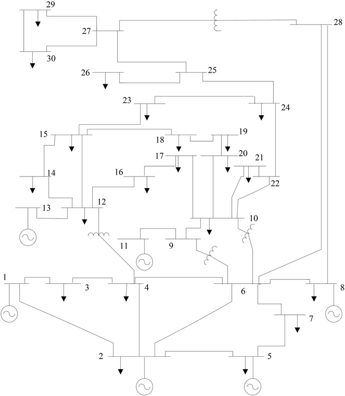
FIGURE 1. Single line diagram of IEEE 30-bus test system.

Table 1 summarizes optimal solutions obtained by MGBLFA for all possible configurations of the 30-bus power system for 8 cases. The optimal values of decision variables indicate that all the limitations of the problem are satisfied, and the algorithm works well.

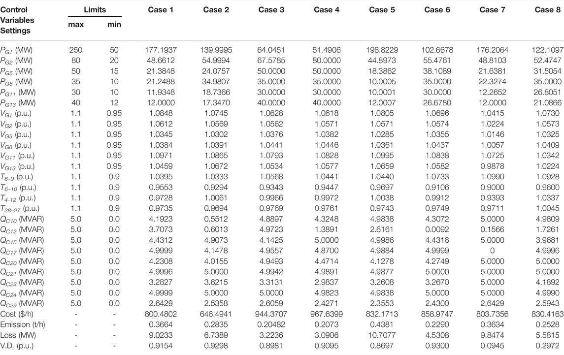
TABLE 1. Optimal control variables of the proposed MGBLFA for determining the lowest cost (best solution) for various test scenarios.

4.1.1 Results of Case 1

The most often employed objective function in OPF studies is the overall producing fuel cost of the entire system, in which each unit has a quadratic function of its own cost structure. Therefore, the objective function indicating the whole cost of fuel production is (Ghasemi et al., 2015b; Mohamed et al., 2017):

Where α_i, b_i and c_i represent the cost coefficients of the ith generator, and NG is the number of total generators. The cost coefficients' values are given in (Mohamed et al., 2017). The minimal fuel cost ($/h), the emission rate (tons/h), the power loss (MW), and the V.D. (p.u.) for the BBDE, BBPSO, LFA, GBLFA, and MGBLFA algorithms are presented in Table 2, and these values are compared to those reported in the current literature. In this example, MGBLFA outperforms the BBDE, BBPSO, LFA, and GBLFA techniques, but BBPSO’s optimum fuel cost value is significantly higher than the other algorithms. As seen in Figure 2, the MGBLFA exhibits smoother curves and a faster convergence rate than other competitive algorithms.

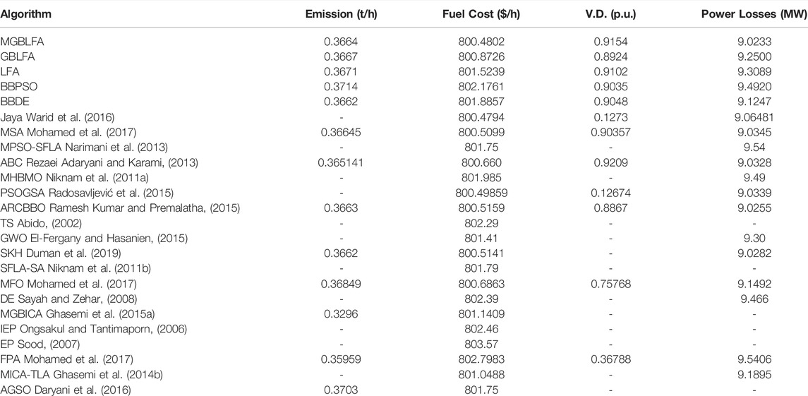
TABLE 2. Comparison of optimal results by algorithms for Case 1.

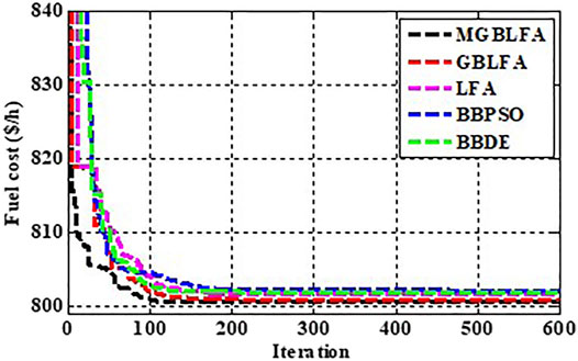
FIGURE 2. Convergence characteristics of the algorithms for Case 1.

4.1.2 Results of Case 2

Thermal power plants may run on natural gas and oil in certain situations. Thus, the fuel cost function is segmented into piecewise quadratic cost functions depending on the quantity and consumed fuels. Thus, the cost of creating fuel when many fuels are represented by a specific goal for a single generator may be given by (42) (Ghasemi et al., 2015a).

Where k is the fuel option, in this case, the total fuel cost function can be calculated as follows:

The data for units that operate on several fuel types was derived from (Mohamed et al., 2017). The optimal solution achieved with MGBLFA is listed in Table 1. In addition, Table 3 shows how this outcome relates to the findings of other algorithms and how it compares to other techniques published in the literature. This table indicates that MGBLFA surpasses all optimization techniques tried to solve OPF in this situation. Figure 3 depicts the development of the goal function for Case 2 across iterations using algorithms.

TABLE 3. Comparison of optimal results by algorithms for Case 2.

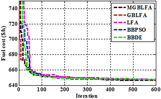
FIGURE 3. Convergence characteristics of the algorithms for case 2.

4.1.3 Results of Case 3

In this example, the aim is to decrease the emission of two significant pollutants, namely NOX and SOX, which may be expressed as follows (Mohamed et al., 2017):

Where F_Ei represents the emission of the ith generator. ${\gamma }_i$, ${\beta }_i$, ${\xi }_i$ and ${\lambda }_i$ are the emission coefficients of the ith generator, while ${\gamma }_i$ (ton/h MW²), ${\beta }_i$ (ton/h MW), and ${\alpha }_i$ (ton/h) are related to SOX. The ${\xi }_i$ (ton/h), ${\lambda }_i$ (1/MW) are related to NOX, respectively (Ghasemi et al., 2014a).

The outcomes of the algorithms are summarized in Table 4. The usefulness of algorithms is highly dependent on the nature of the goal function. Figure 4 illustrates the evolution of the emission cost across the iterations. The MSA (Mohamed et al., 2017), the ARCBBO (Ramesh Kumar and Premalatha, 2015), the GBLFA, and the MGBLFA arrived at the optimal final solution.

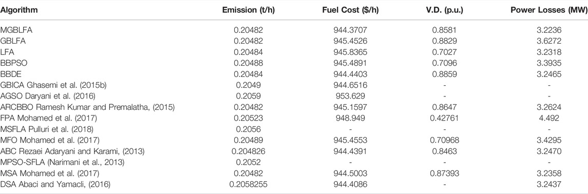
TABLE 4. Comparison of optimal results by algorithms for case 3.

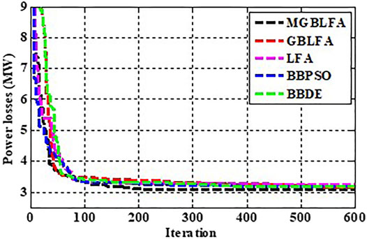
FIGURE 4. Convergence characteristics of the algorithms for Case 3.

4.1.4 Results of Case 4

The purpose of this instance was to minimize the active power loss on each transmission line by optimizing the following objective function (Mohamed et al., 2017):

Where P_Loss is the total active power losses of the transmission network. g_ij is the conductance of branch ij, δ_ij phase difference of voltages between bus i and bus j.

The suggested MGBLFA reduced the objective function and produced outstanding findings compared to those previously described in the works (see Table 5). Figure 5 illustrates the power loss convergence characteristics in different algorithms. Algorithms behave similarly to Case 1. One reason for this could be that the optimization problem forms of both situations are similar.

TABLE 5. Comparison of optimal results by algorithms for Case 4.

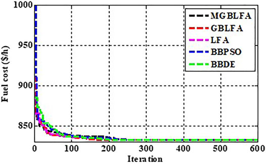
FIGURE 5. Convergence characteristics of the algorithms for Case 4.

4.1.5 Results of Case 5

The valve-point effect (VPE) must be included for a more accurate and exact simulation of the fuel cost function. The fuel-cost functions of generating units equipped with multi-valve steam turbines display more variance. Opening the valves in multi-valve steam turbines creates a ripple effect (Sood, 2007. This impact is significant since a huge steam plant’s real cost curve function is non-linear, not continuous (Sood, 2007). As a result, the objective function expressing the overall cost of producing gasoline while accounting for the valve-point impact is as follows (Mohamed et al., 2017):

Where, d_i and e_i are the coefficients that represent the valve-point loading effect.

The ultimate results of MGBLFA are superior yet comparable to those of other algorithms, as shown in Table 6. Furthermore, Figure 6 illustrates the convergence characteristics of the utilized algorithms for Case 5. The results indicate the better convergence behavior of the proposed algorithm concerning other competitive algorithms.

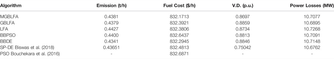
TABLE 6. Comparison of optimal results by algorithms for Case 5.

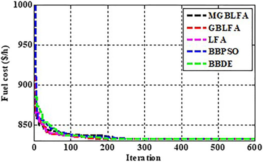
FIGURE 6. Convergence characteristics of the algorithms for Case 5.

4.1.6 Results of Case 6

This case is designed to reduce both fuel costs and transmission losses. Accordingly, the cost function can be depicted as follows:

Where, the value of loss factor λp is chosen as 40, the same as in (Biswas et al., 2018).

The ideal objective function values for this example are presented in Table 7 demonstrating that the MGBLFA and a DE integrated with the constraint handling technique SF (superiority of feasible solutions) (SF-DE) (Biswas et al., 2018) executed better than the other algorithms.

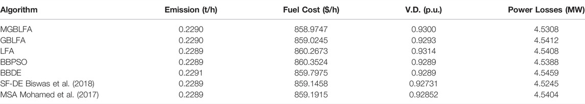
TABLE 7. Comparison of optimal results by algorithms for Case 6.

4.1.7 Results of Case 7

In this situation, multi-objective optimization is used, with the aim of minimizing the fuel cost while enhancing the voltage profile, as specified in Eq. 48. The factor λv is set to 100, as in (Biswas et al., 2018). As seen in Table 8, the voltage magnitude variations are significantly decreased, although the overall fuel cost is raised when compared to the prior example.

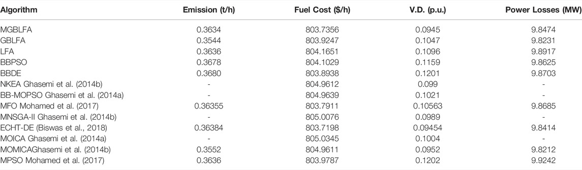
TABLE 8. Comparison of optimal results by algorithms for Case 7.

4.1.8 Results of Case 8

The purpose of this instance is to minimize four conflicting objectives simultaneously: pollution, losses, fuel expense, and voltage variations. Thus, the goal function is to simultaneously solve instances 3, 4, and 6, which may be expressed as follows:

The weight factors are selected as λv = 21, λp = 22 and λe = 19 to balance among the problem different objectives. The evaluation of optimal results obtained by different algorithms for this situation is shown in Table 9, demonstrating that the MGBLFA algorithm is an appropriate and dependable solution to the MOOPF problem in power systems.

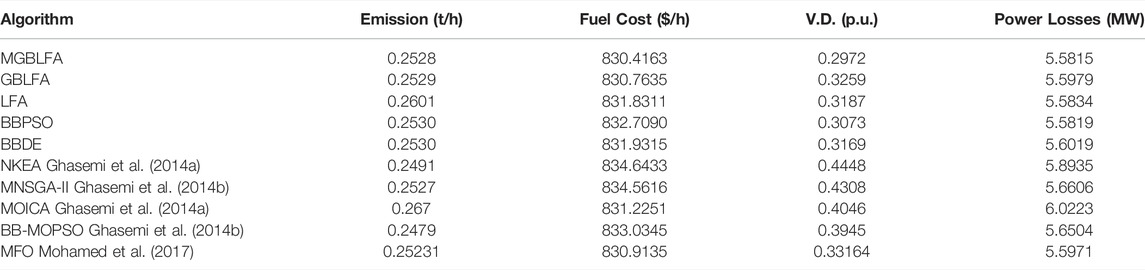
TABLE 9. Comparison of optimal results by algorithms for Case 8.

4.2 OPF for Renewable Power Integrated Systems

4.2.1 Results of Case 9

In this case, the production schedule for all generators, including thermal and renewable sources, is optimally defined using the proposed algorithm to minimize overall generating costs, $TC,$ as defined in Eq. 50.

As with Case 1, the cost coefficients are the same as in Table 10. Table 11 summarizes the optimization of all decision variables, reactive generator (Q) power, the overall cost of generation and other relevant computed metrics. The voltage V_i in the tables refers to ith bus voltage. Pws,₁ means the scheduling power of the wind generator WG1 and furthermore. The minimal generation costs that can be reached by generation schedules mentioned in the table are BBDE, BBPSO, LFA, GBLFA and MGBLFA, correspondingly at $783,0573, 783,0301, 782,2258, 782,0752 and 781,3930 $/h. The suggested method for MGBLFA can clearly discover the best answer for the same circumstance as BBDE, BBPSO, LFA, and GBLFA.

TABLE 10. PDF parameters of wind power and solar PV plants.

TABLE 11. The variables optimal values obtained by algorithms for Case 9.

4.2.2 Results of Case 10

In recent years, several governments have been placing considerable pressure on the whole energy industry to lower carbon emissions because of global warming (Biswas et al., 2017). Carbon tax (C_tax) is levied on each unit of emission of greenhouse gases to stimulate investment in greener types of power such as wind and solar. The total generation cost as well as emission cost (in $/h), $TCE$ , can be defined as follows:

This study reduces the entire cost of generating, including carbon tax on emissions from traditional thermal power plants. The tax on carbon is supposed to be $20/ton (Reddy et al., 2014a). Given that winds and solar energy are clean, carbon tax components will encourage the expansion of these sources. Table 10 shows the optimum generating schedule, reactive power generator, total costs of production (including carbon tax) and other computed factors. In the case of the carbon tax in Case 10, it is noted that the penetration of solar as well as wind energy is more than in Case 9, and no emission penalty is charged by any algorithm. The degree to which renewable sources are optimized relies on the amounts of emissions and the rate of a carbon price applied (Biswas et al., 2017). In OPF, the load-bus voltage limit is especially essential, as load-bus operating voltages are frequently close to their limits. The load bus tension should be kept in our study between 0.95 and 1.05 p.u.

As shown in Table 12, a better carbon tax than the other four adopted is the suggested MGBLFA approach, which is $18,1416/h. Operating more than the suggested approach, BBDE, BBPSO, LFA, and GBLFA have an overall cost target of $792,7096, 793,3920, 793,1464 and 792,7272/h. It is, therefore, possible to conclude that the suggested MGBLFA procedure is quite successful in reducing the IEEE 30-bus system’s overall cost target.

TABLE 12. The variables optimal values obtained by algorithms for Case 10.

4 Discussions

Table 13 presents the end outcomes following 30 runs for each method based upon the best, average, and worst output features and the average simulation duration for every single goal optimizing function. In particular, the suggested MGBLFA method is virtually simultaneously more efficient and optimized than the original LFA algorithm. The overall reliability of the proposal MGBLFA approach can be detected clearly and accurately when comparing the four established BBDE, BBPSO, LFA, and GBLFA methods, as roughly all the outputs of the proposed MGBLFA technique are higher than that of those techniques. In addition, the voltage profile of the load buses corresponding to the best solution obtained by the proposed algorithm is shown in Figure 7. As can be seen, in all ten cases, the voltage magnitudes remain between the upper and lower bounds.

TABLE 13. Comparison of optimal results by the optimization algorithms for single-objective functions.

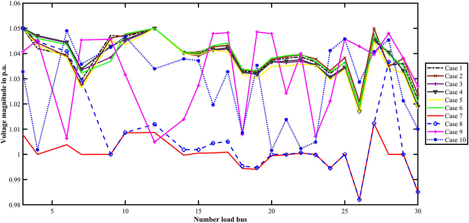
FIGURE 7. Voltage profile of the system for ten cases obtained by the proposed algorithm.

5 Conclusion

The aim of this work was to address the OPF of the systems integrated with wind and solar energy resources to optimize various objective functions such as fuel and operational costs, emission, loss, and voltage deviation. An enhanced Levy-flight firefly algorithm (LFA) method, namely the GBLFA algorithm, and its modified version, i.e., MGBLFA were developed to solve the OPF problem. Then, the performance of the proposed algorithm was tested on the basic IEEE 30-bus tests system without renewable energy integration, and the optimal results were compared with other state-of-the-art algorithms. In this problem, control variables such as transformer tap setting, generator outputs and reactive power generators, or generator voltages, were optimally selected without any violations in the constraints, which proved the accuracy and validity of the proposed algorithm. Compared with all prior research, the suggested GBLFA and MGBLFA algorithms were shown to have effective and trustworthy outcomes for the various OPF problems in IEEE 30-bus test system.

Moreover, wind and solar power generation units were considered in the OPF problem. First, the uncertainties of wind and solar radiations were modeled using Weibull and lognormal PDFs, respectively. After that, the OPF cost function was modified to incorporate the influences of renewable generations. This cost function included the fuel cost of thermal power plants, the cost of the carbon tax on emissions from traditional thermal power plants, the direct costs of the wind/solar, the reserve or overestimation costs, and the penalty costs. The simulation results of the cases with wind and solar power penetrations demonstrated the total cost-benefit of these resources in the OPF problem. The level of renewable power generation is influenced by some constraints such as voltage limits and the value of carbon tax. An increase in carbon taxes will increase the share of renewable power generation. Furthermore, the superiority of the proposed algorithm was investigated and verified in comparison to other algorithms in Cases 9 and 10 for solving OPF problems with renewables. In future work, a stochastic multiobjective model of the OPF problem in the presence of renewable power generations will be developed.

Data Availability Statement

The raw data supporting the conclusion of this article will be made available by the authors, without undue reservation.

Author Contributions

AA: Conceptualization, methodology, software, validation, formal analysis, investigation, writing original draft, reviewing, editing, visualization, and supervision. All authors have read and agreed to the published version of the manuscript.

Conflict of Interest

The author declares that the research was conducted in the absence of any commercial or financial relationships that could be construed as a potential conflict of interest.

Publisher’s Note

All claims expressed in this article are solely those of the authors and do not necessarily represent those of their affiliated organizations, or those of the publisher, the editors and the reviewers. Any product that may be evaluated in this article, or claim that may be made by its manufacturer, is not guaranteed or endorsed by the publisher.

Acknowledgments

The author would like to thank the Deanship of Scientific Research at Majmaah University for supporting this work under Project Number No. R-2022-134.

References

Abaci, K., and Yamacli, V. (2016). Differential Search Algorithm for Solving Multi-Objective Optimal Power Flow Problem. Int. J. Electr. Power & Energy Syst. 79, 1–10. doi:10.1016/j.ijepes.2015.12.021
Abido, M. A. (2002). Optimal Power Flow Using Tabu Search Algorithm. Electr. Power Components Syst. 30 (5), 469–483. doi:10.1080/15325000252888425
Akbari, E. (2022). Optimal Power Flow via Teaching-Learning-Studying-Based Optimization Algorithm. Electr. Power Components Syst. 49 (6–7), 584–601. doi:10.1080/15325008.2021.1971331
Ayan, K., Kılıç, U., and Baraklı, B. (2015). Chaotic Artificial Bee Colony Algorithm Based Solution of Security and Transient Stability Constrained Optimal Power Flow. Int. J. Electr. Power & Energy Syst. 64, 136–147. doi:10.1016/j.ijepes.2014.07.018
Bentouati, B., Khelifi, A., Shaheen, A. M., and El-Sehiemy, R. A. (2021). An Enhanced Moth-Swarm Algorithm for Efficient Energy Management Based Multi Dimensions OPF Problem. J. Ambient. Intell. Hum. Comput. 12 (10), 9499–9519. doi:10.1007/s12652-020-02692-7
Biswas, P. P., Suganthan, P. N., and Amaratunga, G. A. J. (2017). Optimal Power Flow Solutions Incorporating Stochastic Wind and Solar Power. Energy Convers. Manag. 148, 1194–1207. doi:10.1016/j.enconman.2017.06.071
Biswas, P. P., Suganthan, P. N., Mallipeddi, R., and Amaratunga, G. A. J. (2018). Optimal Power Flow Solutions Using Differential Evolution Algorithm Integrated with Effective Constraint Handling Techniques. Eng. Appl. Artif. Intell. 68, 81–100. doi:10.1016/j.engappai.2017.10.019
Bouchekara, H. R. E. H., Chaib, A. E., Abido, M. A., and El-Sehiemy, R. A. (2016). Optimal Power Flow Using an Improved Colliding Bodies Optimization Algorithm. Appl. Soft Comput. 42, 119–131. doi:10.1016/j.asoc.2016.01.041
Chaib, A. E., Bouchekara, H. R. E. H., Mehasni, R., and Abido, M. A. (2016). Optimal Power Flow with Emission and Non-smooth Cost Functions Using Backtracking Search Optimization Algorithm. Int. J. Electr. Power & Energy Syst. 81, 64–77. doi:10.1016/j.ijepes.2016.02.004
Daghan, I. H., Gencoglu, M. T., and Özdemır, M. T. (2021). “Chaos Embedded Particle Swarm Optimization Technique for Solving Optimal Power Flow Problem,” in 2021 18th International Multi-Conference on Systems, Signals & Devices (SSD). IEEE, 725–731. doi:10.1109/ssd52085.2021.9429520
Daryani, N., Hagh, M. T., and Teimourzadeh, S. (2016). Adaptive Group Search Optimization Algorithm for Multi-Objective Optimal Power Flow Problem. Appl. Soft Comput. 38, 1012–1024. doi:10.1016/j.asoc.2015.10.057
Das, S., and Suganthan, P. N. (2010). Differential Evolution: A Survey of the State-Of-The-Art. IEEE Trans. Evol. Comput. 15 (1), 4–31. doi:10.1109/TEVC.2010.2059031
Dasgupta, K., Roy, P. K., and Mukherjee, V. (2020). Power Flow Based Hydro-Thermal-Wind Scheduling of Hybrid Power System Using Sine Cosine Algorithm. Electr. Power Syst. Res. 178, 106018. doi:10.1016/j.epsr.2019.106018
Dash, S. P., Subhashini, K. R., and Chinta, P. (2022). Development of a Boundary Assigned Animal Migration Optimization Algorithm and its Application to Optimal Power Flow Study. Expert Syst. Appl. 200, 116776. doi:10.1016/j.eswa.2022.116776
Dhivya, S., Arul, R., and Padmanathan, K. (2021). “Delicate Flower Pollination Algorithm for Optimal Power Flow,” in Advances in Smart Grid Technology (Springer), 275–289. doi:10.1007/978-981-15-7241-8_20
Dubey, H. M., Pandit, M., and Panigrahi, B. K. (2015). Hybrid Flower Pollination Algorithm with Time-Varying Fuzzy Selection Mechanism for Wind Integrated Multi-Objective Dynamic Economic Dispatch. Renew. Energy 83, 188–202. doi:10.1016/j.renene.2015.04.034
Duman, S., Li, J., and Wu, L. (2021). AC Optimal Power Flow with Thermal-Wind-Solar-Tidal Systems Using the Symbiotic Organisms Search Algorithm. IET Renew. Power Gener. 15 (2), 278–296. doi:10.1049/rpg2.12023
Duman, S., Wu, L., and Li, J. (2019). “Moth Swarm Algorithm Based Approach for the ACOPF Considering Wind and Tidal Energy,” in The International Conference on Artificial Intelligence and Applied Mathematics in Engineering (Springer), 830–843.
El-Fergany, A. A., and Hasanien, H. M. (2015). Single and Multi-Objective Optimal Power Flow Using Grey Wolf Optimizer and Differential Evolution Algorithms. Electr. Power Components Syst. 43 (13), 1548–1559. doi:10.1080/15325008.2015.1041625
El-Sehiemy, R. A. (2022). A Novel Single/multi-Objective Frameworks for Techno-Economic Operation in Power Systems Using Tunicate Swarm Optimization Technique. J. Ambient Intell. Humaniz. Comput. 13 (2), 1–19. doi:10.1007/s12652-021-03622-x
Elattar, E. E. (2019). Optimal Power Flow of a Power System Incorporating Stochastic Wind Power Based on Modified Moth Swarm Algorithm. IEEE Access 7, 89581–89593. doi:10.1109/access.2019.2927193
Farsani, E. A., and Zare, M. (2021). Stochastic Multi-Objective Distribution Network Reconfiguration Considering Wind Turbines. AUT J. Electr. Eng. 53 (1), 11. doi:10.22060/EEJ.2021.19203.5384
Ghasemi, M., Ghavidel, S., Rahmani, S., Roosta, A., and Falah, H. (2014a). A Novel Hybrid Algorithm of Imperialist Competitive Algorithm and Teaching Learning Algorithm for Optimal Power Flow Problem with Non-smooth Cost Functions. Eng. Appl. Artif. Intell. 29, 54–69. doi:10.1016/j.engappai.2013.11.003
Ghasemi, M., Ghavidel, S., Ghanbarian, M. M., Gharibzadeh, M., and Azizi Vahed, A. (2014b). Multi-objective Optimal Power Flow Considering the Cost, Emission, Voltage Deviation and Power Losses Using Multi-Objective Modified Imperialist Competitive Algorithm. Energy 78, 276–289. doi:10.1016/j.energy.2014.10.007
Ghasemi, M., Ghavidel, S., Gitizadeh, M., and Akbari, E. (2015a). An Improved Teaching-Learning-Based Optimization Algorithm Using Lévy Mutation Strategy for Non-Smooth Optimal Power Flow. Int. J. Electr. Power & Energy Syst. 65, 375–384. doi:10.1016/j.ijepes.2014.10.027
Ghasemi, M., Ghavidel, S., Ghanbarian, M. M., and Gitizadeh, M. (2015b). Multi-objective Optimal Electric Power Planning in the Power System Using Gaussian Bare-Bones Imperialist Competitive Algorithm. Inf. Sci. 294, 286–304. doi:10.1016/j.ins.2014.09.051
Güçyetmez, M., and Çam, E. (2016). A New Hybrid Algorithm with Genetic-Teaching Learning Optimization (G-TLBO) Technique for Optimizing of Power Flow in Wind-Thermal Power Systems. Electr. Eng. 98 (2), 145–157. doi:10.1007/s00202-015-0357-y
Gupta, S., Kumar, N., and Srivastava, L. (2021). Solution of Optimal Power Flow Problem Using Sine-Cosine Mutation Based Modified Jaya Algorithm: a Case Study. Energy Sources, Part A Recovery, Util. Environ. Eff. 1–24. doi:10.1080/15567036.2021.1957043
Hassan, M. H., Elsayed, S. K., Kamel, S., Rahmann, C., and Taha, I. B. M. (2022). Developing Chaotic Bonobo Optimizer for Optimal Power Flow Analysis Considering Stochastic Renewable Energy Resources. Int. J. Energy Res. 1–35. doi:10.1002/er.7928
He, X., Wang, W., Jiang, J., and Xu, L. (2015). An Improved Artificial Bee Colony Algorithm and its Application to Multi-Objective Optimal Power Flow. Energies 8 (4), 2412–2437. doi:10.3390/en8042412
Home-Ortiz, J. M., De Oliveira, W. C., and Mantovani, J. R. S. (2021). Optimal Power Flow Problem Solution through a Matheuristic Approach. IEEE Access 9, 84576–84587. doi:10.1109/access.2021.3087626
Jabr, R. A., and Pal, B. C. (2008). Intermittent Wind Generation in Optimal Power Flow Dispatching. IET Generation, Transm. Distribution 3 (1), 66–74. doi:10.1049/iet-gtd:20080273
Jain, L., and Katarya, R. (2019). Discover Opinion Leader in Online Social Network Using Firefly Algorithm. Expert Syst. Appl. 122, 1–15. doi:10.1016/j.eswa.2018.12.043
Jebaraj, L., and Sakthivel, S. (2022). A New Swarm Intelligence Optimization Approach to Solve Power Flow Optimization Problem Incorporating Conflicting and Fuel Cost Based Objective Functions’. e-Prime-Advances Electr. Eng. Electron. Energy 2, 100031. doi:10.1016/j.prime.2022.100031
Jeddi, B., Einaddin, A. H., and Kazemzadeh, R. (2016). Optimal Power Flow Problem Considering the Cost, Loss, and Emission by Multi-Objective Electromagnetism-like Algorithm. IEEE, 38–45. doi:10.1109/ctpp.2016.7482931
Kamel, S., Ebeed, M., and Jurado, F. (2021). An Improved Version of Salp Swarm Algorithm for Solving Optimal Power Flow Problem. Soft Comput. 25 (5), 4027–4052. doi:10.1007/s00500-020-05431-4
Kavousi-Fard, A., Samet, H., and Marzbani, F. (2014). A New Hybrid Modified Firefly Algorithm and Support Vector Regression Model for Accurate Short Term Load Forecasting. Expert Syst. Appl. 41 (13), 6047–6056. doi:10.1016/j.eswa.2014.03.053
Kennedy, J. (2003). “Bare Bones Particle Swarms,” in Proceedings of the 2003 IEEE Swarm Intelligence Symposium. SIS’03 (Cat. No. 03EX706) (IEEE), 80–87.
Kennedy, J., and Eberhart, R. (1995). “Particle Swarm Optimization,” in Proceedings of ICNN’95-international conference on neural networks. IEEE, 1942–1948.
Khorsandi, A., Hosseinian, S. H., and Ghazanfari, A. (2013). Modified Artificial Bee Colony Algorithm Based on Fuzzy Multi-Objective Technique for Optimal Power Flow Problem. Electr. Power Syst. Res. 95, 206–213. doi:10.1016/j.epsr.2012.09.002
Kusakana, K. (2016). Optimal Scheduling for Distributed Hybrid System with Pumped Hydro Storage. Energy Convers. Manag. 111, 253–260. doi:10.1016/j.enconman.2015.12.081
Langari, R. K., Sardar, S., Amin Mousavi, S. A., and Radfar, R. (2020). Combined Fuzzy Clustering and Firefly Algorithm for Privacy Preserving in Social Networks. Expert Syst. Appl. 141, 112968. doi:10.1016/j.eswa.2019.112968
Li, S., Gong, W., Wang, L., and Gu, Q. (2022). Multi-objective Optimal Power Flow with Stochastic Wind and Solar Power. Appl. Soft Comput. 114, 108045. doi:10.1016/j.asoc.2021.108045
Li, S., Gong, W., Wang, L., Yan, X., and Hu, C. (2020). Optimal Power Flow by Means of Improved Adaptive Differential Evolution. Energy 198, 117314. doi:10.1016/j.energy.2020.117314
Ma, R. (2019). Multi-objective Dynamic Optimal Power Flow of Wind Integrated Power Systems Considering Demand Response. CSEE J. Power Energy Syst. 5 (4), 466–473. doi:10.17775/cseejpes.2017.00280
Mahdad, B., Srairi, K., and Bouktir, T. (2010). Optimal Power Flow for Large-Scale Power System with Shunt FACTS Using Efficient Parallel GA. Int. J. Electr. Power & Energy Syst. 32 (5), 507–517. doi:10.1016/j.ijepes.2009.09.013
Mishra, S., Mishra, Y., and Vignesh, S. (2011). “Security Constrained Economic Dispatch Considering Wind Energy Conversion Systems,” in 2011 IEEE Power and Energy Society General Meeting. IEEE, 1–8.
Mohamed, A.-A. A., Mohamed, Y. S., El-Gaafary, A. A. M., and Hemeida, A. M. (2017). Optimal Power Flow Using Moth Swarm Algorithm. Electr. Power Syst. Res. 142, 190–206. doi:10.1016/j.epsr.2016.09.025
Mostafa, A., Ebeed, M., Kamel, S., and Abdel-Moamen, M. A. (2021). Optimal Power Flow Solution Using Levy Spiral Flight Equilibrium Optimizer with Incorporating CUPFC. IEEE Access 9, 69985–69998. doi:10.1109/access.2021.3078115
Narimani, M. R., Azizipanah-Abarghooee, R., Zoghdar-Moghadam-Shahrekohne, B., and Gholami, K. (2013). A Novel Approach to Multi-Objective Optimal Power Flow by a New Hybrid Optimization Algorithm Considering Generator Constraints and Multi-Fuel Type. Energy 49, 119–136. doi:10.1016/j.energy.2012.09.031
Nguyen, T. T. (2019). A High Performance Social Spider Optimization Algorithm for Optimal Power Flow Solution with Single Objective Optimization. Energy 171, 218–240. doi:10.1016/j.energy.2019.01.021
Niknam, T., Azizipanah-Abarghooee, R., Zare, M., and Bahmani-Firouzi, B. (2013). Reserve Constrained Dynamic Environmental/Economic Dispatch: A New Multiobjective Self-Adaptive Learning Bat Algorithm. IEEE Syst. J. 7 (4), 763–776. doi:10.1109/jsyst.2012.2225732
Niknam, T., Narimani, M. r., Jabbari, M., and Malekpour, A. R. (2011a). A Modified Shuffle Frog Leaping Algorithm for Multi-Objective Optimal Power Flow. Energy 36 (11), 6420–6432. doi:10.1016/j.energy.2011.09.027
Niknam, T., Narimani, M. R., Aghaei, J., Tabatabaei, S., and Nayeripour, M. (2011b). Modified Honey Bee Mating Optimisation to Solve Dynamic Optimal Power Flow Considering Generator Constraints. IET Gener. Transm. Distrib. 5 (10), 989. doi:10.1049/iet-gtd.2011.0055
Omran, M. G. H., Engelbrecht, A. P., and Salman, A. (2009). Bare Bones Differential Evolution. Eur. J. Operational Res. 196 (1), 128–139. doi:10.1016/j.ejor.2008.02.035
Ongsakul, W., and Tantimaporn, T. (2006). Optimal Power Flow by Improved Evolutionary Programming. Electr. Power Components Syst. 34 (1), 79–95. doi:10.1080/15325000691001458
Panda, A., Tripathy, M., Barisal, A. K., and Prakash, T. (2017). A Modified Bacteria Foraging Based Optimal Power Flow Framework for Hydro-Thermal-Wind Generation System in the Presence of STATCOM. Energy 124, 720–740. doi:10.1016/j.energy.2017.02.090
Panda, A., and Tripathy, M. (2014). Optimal Power Flow Solution of Wind Integrated Power System Using Modified Bacteria Foraging Algorithm. Int. J. Electr. Power & Energy Syst. 54, 306–314. doi:10.1016/j.ijepes.2013.07.018
Panda, A., and Tripathy, M. (2015). Security Constrained Optimal Power Flow Solution of Wind-Thermal Generation System Using Modified Bacteria Foraging Algorithm. Energy 93, 816–827. doi:10.1016/j.energy.2015.09.083
Pravina, P., Babu, M. R., and Kumar, A. R. (2021). Solving Optimal Power Flow Problems Using Adaptive Quasi-Oppositional Differential Migrated Biogeography-Based Optimization. J. Electr. Eng. Technol. 16 (4), 1891–1903. doi:10.1007/s42835-021-00739-z
Pulluri, H., Naresh, R., and Sharma, V. (2018). A Solution Network Based on Stud Krill Herd Algorithm for Optimal Power Flow Problems. Soft Comput. 22 (1), 159–176. doi:10.1007/s00500-016-2319-3
Radosavljević, J., Klimenta, D., Jevtić, M., and Arsić, N. (2015). Optimal Power Flow Using a Hybrid Optimization Algorithm of Particle Swarm Optimization and Gravitational Search Algorithm. Electr. Power Components Syst. 43 (17), 1958–1970. doi:10.1080/15325008.2015.1061620
Ramesh Kumar, A., and Premalatha, L. (2015). Optimal Power Flow for a Deregulated Power System Using Adaptive Real Coded Biogeography-Based Optimization. Int. J. Electr. Power & Energy Syst. 73, 393–399. doi:10.1016/j.ijepes.2015.05.011
Reddy, S., Bijwe, P. R., and Abhyankar, A. R. (2014a). Faster Evolutionary Algorithm Based Optimal Power Flow Using Incremental Variables. Int. J. Electr. Power & Energy Syst. 54, 198–210. doi:10.1016/j.ijepes.2013.07.019
Reddy, S., Bijwe, P. R., and Abhyankar, A. R. (2014b). Real-time Economic Dispatch Considering Renewable Power Generation Variability and Uncertainty over Scheduling Period. IEEE Syst. J. 9 (4), 1440–1451. doi:10.1109/JSYST.2014.2325967
Rezaei Adaryani, M., and Karami, A. (2013). Artificial Bee Colony Algorithm for Solving Multi-Objective Optimal Power Flow Problem. Int. J. Electr. Power & Energy Syst. 53, 219–230. doi:10.1016/j.ijepes.2013.04.021
Roy, R., and Jadhav, H. T. (2015). Optimal Power Flow Solution of Power System Incorporating Stochastic Wind Power Using Gbest Guided Artificial Bee Colony Algorithm. Int. J. Electr. Power & Energy Syst. 64, 562–578. doi:10.1016/j.ijepes.2014.07.010
Saeidi, M., Niknam, T., Aghaei, J., and Zare, M. (2019). Multi-Objective Coordination of Local and Centralized Volt/Var Control with Optimal Switch and Distributed Generations Placement. J. Intell. Fuzzy Syst. 36 (6), 6605–6617. doi:10.3233/jifs-18631
Sánchez, D., Melin, P., and Castillo, O. (2017). Optimization of Modular Granular Neural Networks Using a Firefly Algorithm for Human Recognition. Eng. Appl. Artif. Intell. 64, 172–186. doi:10.1016/j.engappai.2017.06.007
Sayah, S., and Zehar, K. (2008). Modified Differential Evolution Algorithm for Optimal Power Flow with Non-smooth Cost Functions. Energy Convers. Manag. 49 (11), 3036–3042. doi:10.1016/j.enconman.2008.06.014
Shaheen, A. M., El-Sehiemy, R. A., Alharthi, M. M., Ghoneim, S. S. M., and Ginidi, A. R. (2021). Multi-objective Jellyfish Search Optimizer for Efficient Power System Operation Based on Multi-Dimensional OPF Framework. Energy 237, 121478. doi:10.1016/j.energy.2021.121478
Shayeghi, H., and Ghasemi, A. (2014). A Modified Artificial Bee Colony Based on Chaos Theory for Solving Non-convex Emission/economic Dispatch. Energy Convers. Manag. 79, 344–354. doi:10.1016/j.enconman.2013.12.028
Shi, L. (2011). Optimal Power Flow Solution Incorporating Wind Power. IEEE Syst. J. 6 (2), 233–241. doi:10.1109/JSYST.2011.2162896
Singh, R. P., Mukherjee, V., and Ghoshal, S. P. (2016). Particle Swarm Optimization with an Aging Leader and Challengers Algorithm for the Solution of Optimal Power Flow Problem. Appl. Soft Comput. 40, 161–177. doi:10.1016/j.asoc.2015.11.027
Sood, Y. (2007). Evolutionary Programming Based Optimal Power Flow and its Validation for Deregulated Power System Analysis. Int. J. Electr. Power & Energy Syst. 29 (1), 65–75. doi:10.1016/j.ijepes.2006.03.024
Swief, R. A., Hassan, N. M., Hasanien, H. M., Abdelaziz, A. Y., and Kamh, M. Z. (2021). Multi-regional Optimal Power Flow Using Marine Predators Algorithm Considering Load and Generation Variability. IEEE Access 9, 74600–74613. doi:10.1109/access.2021.3081374
Tazvinga, H., Zhu, B., and Xia, X. (2015). Optimal Power Flow Management for Distributed Energy Resources with Batteries. Energy Convers. Manag. 102, 104–110. doi:10.1016/j.enconman.2015.01.015
Vandenbergh, F., and Engelbrecht, A. (2006). A Study of Particle Swarm Optimization Particle Trajectories. Inf. Sci. 176 (8), 937–971. doi:10.1016/j.ins.2005.02.003
Venkateswara Rao, B., and Nagesh Kumar, G. V. (2015). Optimal Power Flow by BAT Search Algorithm for Generation Reallocation with Unified Power Flow Controller. Int. J. Electr. Power & Energy Syst. 68, 81–88. doi:10.1016/j.ijepes.2014.12.057
Wang, G. (2012). A Modified Firefly Algorithm for UCAV Path Planning. Int. J. Hybrid Inf. Technol. 5 (3), 123–144. doi:10.14257/ijhit.2012.5.3.11
Warid, W., Hizam, H., Mariun, N., and Abdul-Wahab, N. (2016). Optimal Power Flow Using the Jaya Algorithm. Energies 9 (9), 678. doi:10.3390/en9090678
Yang, X.-S., Sadat Hosseini, S. S., and Gandomi, A. H. (2012). Firefly Algorithm for Solving Non-convex Economic Dispatch Problems with Valve Loading Effect. Appl. soft Comput. 12 (3), 1180–1186. doi:10.1016/j.asoc.2011.09.017
Yang, X. (2010a). ‘Firefly Algorithm, Lévy Distributions and Global Optimization’, Research And Development In Intelligent Systems XXVI [Preprint]. London, UK: Springer.
Yang, X. (2010b). Firefly Algorithm, Stochastic Test Functions and Design Optimisation. Int. J. bio-inspired Comput. 2 (2), 78–84. doi:10.1504/ijbic.2010.032124
Yao, F., Dong, Z. Y., Meng, K., Xu, Z., Iu, H. H.-C., and Wong, K. P. (2012). Quantum-inspired Particle Swarm Optimization for Power System Operations Considering Wind Power Uncertainty and Carbon Tax in Australia. IEEE Trans. Ind. Inf. 8 (4), 880–888. doi:10.1109/tii.2012.2210431
Zargar, S. F., Farsangi, M. M., and Zare, M. (2020). Probabilistic Multi-Objective State Estimation-Based PMU Placement in the Presence of Bad Data and Missing Measurements. IET Gener. Transm. Distrib. 14 (15), 3042–3051. doi:10.1049/iet-gtd.2019.1317
Zhou, W., Peng, Y., and Sun, H. (2011). Optimal Wind-Thermal Coordination Dispatch Based on Risk Reserve Constraints. Euro. Trans. Electr. Power 21 (1), 740–756. doi:10.1002/etep.474
Keywords: OPF problem, Gaussian bare-bones levy-flight firefly algorithm (GBLFA), modified GBLFA, wind and solar energy systems, nonsmooth cost functions
Citation: Alghamdi AS (2022) Optimal Power Flow of Renewable-Integrated Power Systems Using a Gaussian Bare-Bones Levy-Flight Firefly Algorithm. Front. Energy Res. 10:921936. doi: 10.3389/fenrg.2022.921936
Received: 16 April 2022; Accepted: 29 April 2022;
Published: 26 May 2022.
Edited by:
Ziad M. Ali, Aswan University, EgyptReviewed by:
Emad M. Ahmed, Al Jouf University, Saudi ArabiaPeerapong Uthansakul, Suranaree University of Technology, Thailand
Copyright © 2022 Alghamdi. This is an open-access article distributed under the terms of the Creative Commons Attribution License (CC BY). The use, distribution or reproduction in other forums is permitted, provided the original author(s) and the copyright owner(s) are credited and that the original publication in this journal is cited, in accordance with accepted academic practice. No use, distribution or reproduction is permitted which does not comply with these terms.
*Correspondence: Ali S. Alghamdi, aalghamdi@mu.edu.sa