Prediction of the 3D Distribution of NOx in a Furnace via CFD Data Based on ELM

1 Introduction

Nitrogen oxides (NOx), released by coal-fired power plants, are one of the most harmful air pollutants that tend to seriously impact the air quality and human health. New NOx emission standards in coal-fired power plants list them to be below 100 mg of NO₂/Nm3 at 6% O₂ (dry-basis) (Ministry of Environmental Protection of the PRC, 2011). There are two primary methods to decrease NOx emissions: 1) flue gas denitration and 2) low nitrogen combustion (Fang Wang et al., 2018). Flue gas denitration is a post-treatment method that is performed by adding denitration devices at the tail flue. On the other hand, the low nitrogen combustion method utilizes low NOx burners or fuel/air at the combustion stage. The essence of low nitrogen combustion is to change the temperature field and component distribution in the furnace to reduce NOx formation. However, a lack of means for effective on-line observation of temperature and component distribution hinders the understanding of NOx formation. Rapid and accurate prediction of 3D spatial distribution of NOx has become a necessity in order to control NOx emissions and optimize the combustion process.

Two methods are usually used to obtain the NOx concentration in emissions of the coal-fired power plants: 1) the mechanism-based method and 2) the data-driven method. Computational fluid dynamics (CFD), a mechanism-based method, involves solving the partial differential equations governing the combustion process to simulate it under the given boundary and initial conditions (Dindarloo and Hower, 2015; Boyd and Kent, 1988; Xu et al., 2001). The calculation of NOx emissions through CFD can be divided into two stages. The first stage includes evaluating the 3D spatial distribution of the temperature field, velocity field, and products of combustion in the furnace. The second stage involves NOx distribution evaluation by means of post-processing the already obtained combustion product data. CFD simulations with regards to the NOx spatial distribution mostly investigate the effects of a certain change in the working conditions of a furnace. This may include variations in boiler loads (Dindarloo and Hower, 2015; Boyd and Kent, 1988), swirl arrangements and coal injection modes (Choi et al., 2020), air staging combustion (Zhang et al., 2015; Wang and Zhou, 2020), separated over-fire air (SOFA) ratio and location (Ma et al., 2015), and tilt angles of the burner (Tan et al., 2017). CFD methods can analyze the change in NOx spatial distribution based on different input conditions and the relationships between various parameters. There have also been some improvements over the years with regards to the CFD combustion simulation methods .Zhang et al. (2019) proposed a semi-empirical modeling strategy with the large eddy simulation in which the concentration of CO + H2 substituted CHi, which is difficult to calculate to quantify NO homogenous reduction. The new model can accurately predict different NOx evolution characteristics under various conditions. Secco et al. (2015) coupled a genetic algorithm with CFD calculations to automatically generate optimal boiler configurations for minimizing NOx emissions. CFD simulations can also be used to optimize the combustion process. A drawback of using CFD simulations, however, is that they involve a plethora of complicated calculations which consume a large amount of time.

Another method to predict the NOx distribution is the data-driven method. This method is mainly focused on the NOx emission of the exhaust gas. In this regard, numerous algorithms, including statistical regression (Li et al., 2004; Chunlin Wang et al., 2018), support vector machine (Wei et al., 2013; Zhou et al., 2012; Ahmed et al., 2015; Lv et al., 2013), artificial neural network (ANN) (Chu et al., 2003; Ilamathi et al., 2013; Preeti and Sharad, 2013; Jacob and Tuttll, 2019), and deep learning (Li and Hu, 2020; Yang et al., 2020; Tan et al., 2019; Xie et al., 2020; Kang et al., 2017; Wang et al., 2017) are often used to predict the NOx concentration. Although remarkable achievements have been obtained in this area, the time complexity of support vector machines increases exponentially as the sample size increases. This problem may be attributed to quadratic programming problems. Moreover, the ANN is easy to fall into the local minimum and has the risk of over-fitting. The required data of data-driven modeling are usually collected from the operation and experimental data of power plants. In this regard, scholars have tried to combine CFD techniques with experimental data to predict the NOx distribution in engineering applications (Fang Wang et al., 2018; Yan et al., 2019). Currently, CFD data are mainly used as the supplement of operation data, or it is combined with historical data to obtain comprehensive data on the working conditions. However, it is a challenge to analyze a huge amount of 3D data obtained from CFD simulation. On the other hand, simple NOx prediction of the exhaust gas is not conducive to optimizing combustion parameters and fault analysis.

In this study, a data-driven method is proposed to obtain the 3D NOx distribution based on the extreme learning machine (ELM) method. Then, NOx distribution in the furnace is obtained using CFD simulation. The obtained data are partitioned based on the formation mechanism of NOx in the furnace. Meanwhile, the Pearson coefficient and mutual information (PMI) is used to obtain optimal inputs. Finally, the ELM is applied to establish a 3D NOx distribution model in the furnace, and the feasibility of the method is verified through experiments. The proposed model is expected to obtain the 3D distribution of NOx at any burner tilt angle quickly and accurately and provide a guideline for combustion optimization and NOx emission reduction.

2 Description of the Proposed System

2.1 Boiler Description

In the present study, a 350 MW once-through supercritical boiler is selected as the research object. Figure 1 illustrates the schematic layout of the boiler. The boiler is 58,300 mm high and has a 14,627 × 14.627 mm cross section. Moreover, the depth of the horizontal and tail flue gas duct is 53,200 mm and 68,200 mm, respectively. The boiler adopts a new type of tangential combustion. The main combustion area contains six layers of pulverized coal air chambers and eight layers of auxiliary air chambers. Each pulverized coal–air chamber has four nozzles, which are arranged on the four planes of the water-cooled wall. Four secondary air nozzles are arranged in each auxiliary air chamber to surround it. Moreover, four SOFA layers are installed in the corner above the main combustion area to replenish the required air in the next stage of combustion.

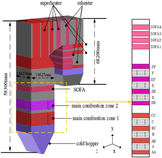
FIGURE 1. Schematic structure and burner arrangement of the studied 350 MW boiler. (A) Boiler structure (B) Arrangement of the burner and the secondary wind.

The main operating parameters at the rated power of the boiler are shown in Table 1. Table 2 shows the chemical composition of the coal.

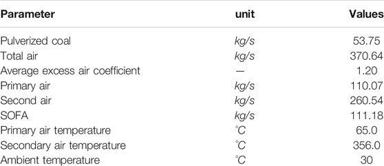
TABLE 1. Main boiler operating parameters at the rated power.

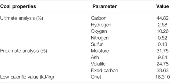
TABLE 2. Proximate and ultimate analyses of pulverized coal.

2.2 Overall Modeling of Modeling

Obtaining the 3D distribution of NOx concentration in the furnace mainly consists of four steps, including CFD simulation, data preprocessing, feature selection, and ELM modeling. The overall modeling process is shown in Figure 2.

Step 1: Input parameters and boundary conditions are set according to the type of the boiler and unit load, and then, CFD simulation is carried out.

Step 2: The 3D distribution data obtained from CFD simulation are preprocessed; then, the data are partitioned into multiple subsets based on the formation mechanism of NOx.

Step 3: Primary data are selected based on the formation mechanism; then, the PMI is combined for feature selection. Finally, variables with high correlation are selected as modeling inputs.

Step 4: Prediction models of the NOx distribution of each subset are established based on the ELM concept. It is worth noting that different subsets have different optimal inputs. Accordingly, multiple NOx prediction models can be obtained for different conditions. Hence, all partial models should be integrated into the final prediction model.

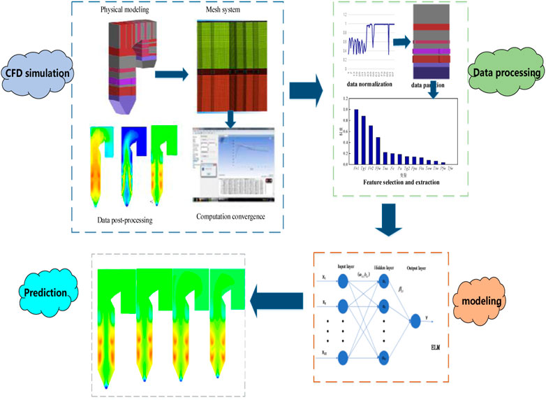
FIGURE 2. Modeling framework to obtain the 3D NO_X distribution in the furnace.

3 Computational Fluid Dynamics Simulation

Generally, CFD simulation consists of three steps, including pre-processing, solving governing equations, and post-processing. The main objective of pre-processing is to prepare the computational domain and generate an appropriate mesh. Figure 1 shows that the calculation domain includes the furnace and horizontal and rear passes. In the present study, structured hexahedral meshes are used for the furnace body, while refined unstructured meshes are used in the combustion zone to ensure the accuracy of calculations. Three mesh resolutions, containing 2.82*10⁶, 3.18*10⁶, and 3.43*10⁶ meshes, are used to perform the grid independence test. Trading off between simulation accuracy and the computational expense, 3.18*10⁶ meshes are used in all simulations.

In this article, Fluent 15.0 software is used to study the behavior of gas-solid two-phase flow and coal combustion. Moreover, the k−ε model is used to solve the gas-phase turbulent equations. Meanwhile, the stochastic tracking model is used in the Euler–Lagrange method to simulate the two-phase flow. In the combustion model, the volatile pyrolyzation model adopts the two-step competitive reaction model, and the diffusion/kinetics model is used to describe char combustion. The discrete ordinates (DO) model is selected to model radiant heat transfer in the furnace. The load, excess air coefficient, coal quality, primary and secondary air distribution, and SOFA are important and affecting parameters in the furnace. The imposed boundary conditions are presented in Table 2.

To verify the CFD model, the simulation results of the 0°tilt angle are compared with plant data at the rated point. Table 3 reveals that the absolute error of the outlet gas temperature (T1) is 6°C, which is equivalent to a relative error of less than 1%. Furthermore, the absolute error of the gas temperature of the platen superheater bottom is 32°C, which is equivalent to a relative error of less than 3%. The relative error of O₂ concentration at the boiler outlet is 5.5%. The performed analyses demonstrate that the CFD model can be applied to simulate combustion accurately.

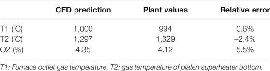
TABLE 3. The comparison between CFD results and experimental plant values.

CFD simulations are carried out for constant operating conditions and different burner tilt angles. In this regard, seven tilt angles (−30°, −20°, −10°, 0°, 10°, 20°, and 30°) are considered, and the concentration of combustion products and the flow field are obtained.

4 3D NOx Emission Prediction Using Extreme Learning Machine

4.1 Data Preprocessing

4.1.1 Data Acquisition and Normalization

First, the outliers should be processed. Based on the physical mechanism, when an abnormal value of temperature or species concentration is achieved, it is set to zero. On the other hand, when an individual node has an extremely higher or lower value than the surrounding nodes, the mean value of surrounding nodes is used for it.

Meanwhile, different variables have different orders of magnitude. The influence of data with high orders can be highlighted in the modeling process, while other data with low numerical values but great influence, such as O₂ concentration, may be ignored. In order to ensure the reliability of the model and training speed, it is necessary to perform a Min-Max data normalization process. This can be mathematically expressed as follows:

where ${\mathit{x}}_{\mathit{i}}$ is the original value, ${\mathit{x}}_{\mathit{i}}^{\mathit{*}}$ is the normalized value, and ${\mathit{x}}_{\mathit{max}}$ and ${\mathit{x}}_{\mathit{min}}$ denote maximum and minimum values, respectively.

4.1.2 Data Partition Based on the NOx Formation Mechanism

The formation of NOx in the furnace is a complex process that involves numerous chemical reactions and thermal phenomena. In a large-scale coal-fired boiler, more than 90% of the total NOx originates from NO (Diez et al., 2017). On the other hand, NO can be divided into three categories, including thermal NOx, fuel NOx, and prompt NOx, according to different formation mechanisms. Studies show that the concentration of prompt NO in conventional burners and furnaces is very low so that it can be ignored in calculations.

Thermal NOx refers to the nitrogen oxide generated by the oxidation of N₂ molecules of the combustion air at high temperatures. In this reaction, NOx is created based on the extended Zeldovich mechanism. The net formation rate of NO can be calculated from the following expression:

To calculate the formation rate of NOx, the concentrations of affecting radicals such as N, O, H, and OH should be determined first. The partial equilibrium method can be used to determine the concentrations of these radicals (United States: Fluent Inc., 2006). In this method, it is assumed that the generation rate and dissipation rate of radicals in a short period of time are equal.

Fuel NOx refers to the oxidation of molecular nitrogen that exists in the fuel structure (e.g., coal here). In this regard, the De Soete mechanism is widely used to determine the formation and depletion of fuel NOx. According to this mechanism, fuel-based N can be classified into volatile N and char N. The formation of fuel NOx is presented in Figure 3. It should be indicated that HCN and NH3 are the main intermediates of volatile N and char N. It is observed that the formation of fuel NOx is mainly affected by the O₂ concentration, fuel type, and char surface density.

FIGURE 3. Chemical reactions that lead to the formation of fuel NOx.

The origin of coordinates of the geometric model is located at the center of the furnace bottom. Axes of coordinates are shown in Figure 1. In order to improve the accuracy of the results and reduce the computational expenses, the data were divided into 11 subsets along the y-direction according to the combustion mechanism. Table 4 indicates that subset 1 refers to the cold ash hopper area. There are two main combustion areas, which are divided into seven burner subsets. Subsets 9 and 10 denote the transition zone and SOFA area, respectively. Moreover, subset 11 refers to the furnace top and the horizontal and tail flue heat transfer zone.

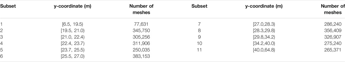
TABLE 4. Partitioned data in the furnace.

4.2 Feature Selection Based on the Pearson Correlation and MI

The selection of input variables directly affects the prediction accuracy, computational expenses, and generalization of the model. In the present study, 21 relevant variables are preselected from CFD simulation data according to the NOx formation mechanism. The input variables of 11 subsets are reselected from 21 relevant variables based on the Pearson coefficient and mutual information (PMI).

In the first step, the PMI variables are determined using Eq. 3. When the correlation coefficient between the two variables is ${\mathit{\rho }}_{{\mathit{x}}_{\mathit{i}}\mathit{,}{\mathit{x}}_{\mathit{j}}}\mathit{>}\mathrm{0}\mathrm{.9}$, one of them can be removed to reduce the dimension of input variables.

The MI-based feature selection method can be applied to obtain the optimal feature by maximizing the joint MI between the input features and the target variable. The joint MI of NOx and related inputs can be defined as follows:

where $\mathit{p}\left({\mathit{x}}_1,{\mathit{x}}_2,\cdots ,{\mathit{x}}_{\mathit{m}}\mathit{,N}{\mathit{O}}_{\mathit{x}}\right)$ is the variable joint distribution, $\mathit{p}\left({\mathit{x}}_1,{\mathit{x}}_2,\cdots ,{\mathit{x}}_{\mathit{m}}\right)$ is the marginal distribution of input variables, and $\mathit{p}\left(\mathit{N}{\mathit{O}}_{\mathit{x}}\right)$ denotes the marginal distribution of NOx.

According to the PMI feature selection, except for three variables (x-, y-, and z-coordinates), seven variables have a relatively high correlation with NOx concentration. These variables are listed in Table 5, according to the correlation intensity. In addition to three coordinate variables, 10 CFD variables of each subset are retained.

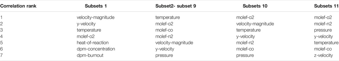
TABLE 5. Feature selection of each subject.

4.3 Obtaining the NO_X Distribution

4.3.1 Extreme Learning Machine

ELM (Huang et al., 2017) is a single hidden layer feedforward neural network (SLFN), which has remarkable properties such as simple structure, fast learning, and superior generalization performance. Accordingly, ELM is widely used in different kinds of dimensional reduction or regression problems. Figure 4 shows the structural block diagram of the ELM network.

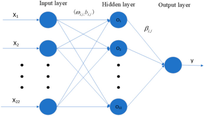
FIGURE 4. Structural diagram of the ELM network.

In an ELM model, $\left(X_i,t_i\right)$, $X_i={\left[{\mathit{x}}_{\mathit{i}1},{\mathit{x}}_{\mathit{i}2},\cdots ,{\mathit{x}}_{\mathit{im}}\right]}^T\in R^n$, and $t_i={\left[{\mathit{t}}_{\mathit{i}1},{\mathit{t}}_{\mathit{i}2},\cdots ,{\mathit{t}}_{\mathit{im}}\right]}^T\in R^m$, are train sets, and $g\left(x\right)$ is the activation function. The output of the ELM can be expressed as follows:

where $j=\mathrm{1,2},\cdots ,L$, and $L$ refers to hidden nodes; ${\mathit{\omega }}_{\mathit{i}}$ is the connection weight between the hidden and the input layers; ${\mathit{\beta }}_{\mathit{i}}$ is the connection weight between the hidden and output layers; ${\mathit{b}}_{\mathit{i}}$ denotes the offset of the i^th hidden layer, and ${\mathit{\omega }}_{\mathit{i}}\cdot {\mathit{x}}_{\mathit{j}}$ is the inner product. When the optimal $\mathit{\beta }$, $\mathit{\omega }$, and $\mathit{b}$, are optimized, then the error reaches zero $\left({\displaystyle \sum }_{j=1}^N{o}_j-t_j=0\right)$. Consequently, Eq. 5 can be rewritten in the form below:

Eq. 6 can also be expressed in the following matrix form:

where $\mathit{H}$ is the neuron output matrix, $\mathit{\beta }$ is the output weight, and $\mathit{T}$ is the output of the neural network. In the ELM algorithm, minimum norm least-squares (LS) are used to solve the SLFN. When the activation function $g\left(x\right)$ is infinitely differentiable, the input weight ${\mathit{\omega }}_{\mathit{i}}$ and hidden layer bias ${\mathit{b}}_{\mathit{i}}$ can be randomly set to t (Huang et al., 2017). The training process of ELM consists of two steps, including random feature mapping and linear parameter solution. In ELM, the hidden layer is initialized randomly through nonlinear mapping functions, and the data are mapped to the feature space. Accordingly, the output weight matrix $\widehat{\beta }$ can be obtained based on the least-squares regression.

where ${\mathit{H}}^{+}$ is the Moore–Penrose generalized inverse of the matrix $\mathit{H}$.

4.3.2 Computational Environment and Parameter Setting

All calculations are carried out in the Python 3.5 environment, installed. Configurations of the PC o Sun program are Windows7 (64 bit) and an Intel Core i5-9400F processor with 2.9 GHz processor speed.

The input weight and bias value are randomly selected according to the performed ELM analysis. “tanh” function is selected as the activation function of ELM, and 100 neurons are considered in the hidden layer.

4.3.3 Description of the Data Set

In this section, CFD simulation is carried out to study variations of the tilt angle of a typical burner at rated power. In order to investigate the NOx distribution at an arbitrary angle, training and test data sets should be constructed. According to PMI correlation analysis, NOx distribution is mainly affected by seven factors. Moreover, there are 22 variables as the inputs of the training set.

The construction rules of the data set are shown in Table 6. Four cases are combined to train the model, and one is used to test it. In this study, the NOx distribution of the upward 10° tilt angle will be predicted.

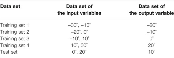
TABLE 6. Construction of the training set and test set.

4.3.4 Performance Metrics

In order to evaluate the prediction performance of models, the mean absolute percentage error (MAPE), root-mean-squared error (RMSE), and correlation coefficient R-square (R²) are used as evaluation indicators. These indicators are defined as follows:

where $\mathit{m}$ is the number of samples in the test set, and ${\overline{\mathit{y}}}_{\mathit{p}}\left(\mathit{i}\right)$ denotes the average value of NO_X distribution. Furthermore, ${\mathit{y}}_{\mathit{c}}$ and ${\mathit{y}}_{\mathit{p}}$ are the calculated and predicted NOx concentrations, respectively.

4.3.5 Prediction of NOx Distribution Based on Extreme Learning Machine

3D distribution of NOx in 11 subsets are modeled respectively adopting the aforementioned ELM model and then are tested by the working condition of the upward 10° burner tilt angle. The predicted results are shown in Table 6.

In this section, it is intended to model the NOx distribution in 11 subsets adopting the ELM model. Then, the results are verified by the experimental data of the upward 10° burner tilt angle. The performance indicators of the predicted results are shown in Table 7.

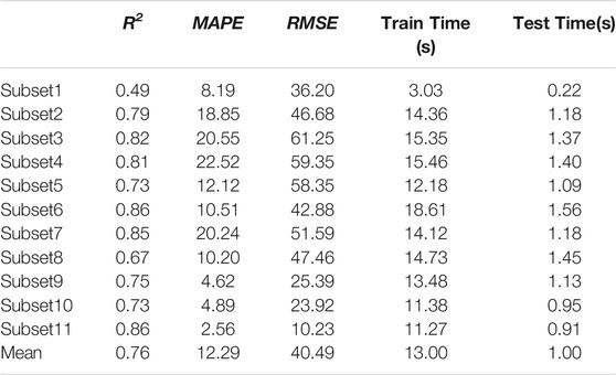
TABLE 7. Performance indicators in different subsets.

Considering the required computational time for CFD simulation, ELM can be applied to rapidly model the flow and obtain the NOx distribution at an arbitrary tilt angle.

Compared with other subsets, R² of subset 1 is relatively small, indicating that the predicted value deviates from the real value. This subset locates in the cold hopper area. Accordingly, the NOx distribution is mainly affected by the ash fall and the combustion in the upper zones. Meanwhile, cold air blowing to the bottom of the furnace affects the field distribution and species concentration. Accordingly, it is an enormous challenge to predict the NOx distribution in this region.

Table 7 indicates that the MAPE of subsets 3, 4, and 7 is about 20%, which is much larger than that of other subsets. These three subsets locate in burner B, burner C, and burner E, respectively. When the burner tilt angle is 10° upward, the combustion center of the lower main combustion zone locates in subsets 3 and 4, and the combustion center of the upper main combustion zone locates in subset 7. Under this circumstance, large turbulent flow and flame fluctuation decreases the prediction accuracy. Figure 5 shows the overall contours of NOx distribution in the studied furnace. It is observed that the NOx concentration in the main combustion zone is relatively high, and the range of variation is large. Consequently, the prediction error is relatively large.

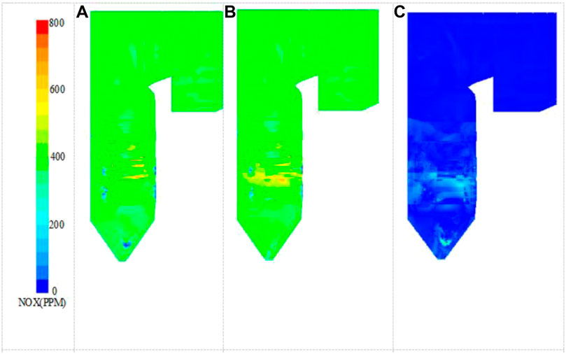
FIGURE 5. Contour of 3D distribution of NO_X. (A) NO_X concentration obtained from CFD simulation (B) NO_X concentration obtained from ELM prediction (C) Prediction error

In subsets 9, 10, and 11, the MAPE and RMSE of the model are small. This is because at the top of the furnace and the horizontal flue, the combustion reaction has ended, and the turbulence disappears. As a result, the distribution of the material composition is stable.

5 Verification of the Algorithm

5.1 Analysis of Feature Selection

To verify the influence of PMI feature selection on the modeling accuracy and efficiency, a comparative study is carried out on the NOx distribution of 11 subspaces. There are 42 input variables before feature selection, including 3 coordinates (x-, y-, and z-coordinates), 19 variables in each known working condition and the burner tilt angle of an unknown working condition. The output is NOx distribution in the desired working condition. Furthermore, there are 22 input variables after PMI feature selection. Three evaluation indicators are used to analyze the modeling effect.

Table 8 shows the mean index indicators of 11 subspaces. It is observed that after feature selection, the mean R² (MR²) increases by 14.5%, while the mean MAPE (MMAPE) and mean RMSE (MRMSE) decrease by 20.9% and 17.2%, respectively. Moreover, mean training time decreases by 3.9 s. It is concluded that predicting the NOx distribution using the PMI feature decreases the prediction data dimension and improves the prediction performance.

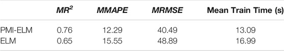
TABLE 8. Statistical indicators of the prediction using different methods.

Considering the high temperature in the combustion zone and the high-temperature gradient around the flame, it is a challenge to simulate the flow accurately. The flue gas flow at the top and tail of the furnace is relatively steady, so the predicted value of NOx distribution is relatively accurate. Figure 6 shows the NOx distribution in the horizontal cross section at four heights of the furnace with an upward burner tilt angle of 10°. It is observed that at the height of 22 m (burner region B), firing circles appear clearly, and the predicted values using the feature extraction are more consistent with the experimental data. At the height of 29 m, airflow rotates and the deviation of the NOx concentration in the furnace center is smaller than that of the case where this feature is not selected. For the SOFA area at 35 m, the prediction accuracy of PMI-ELM is high. At the top of the furnace, the NOx distribution can be accurately predicted regardless of the feature selection. It is inferred that prediction errors mainly appear in the high-temperature zone and the bottom of the furnace. Except for the top region, the prediction performance can be significantly improved using feature extraction.

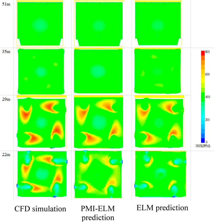
FIGURE 6. Contours of NO_X concentration along the height of the furnace obtained from different methods.

5.2 Comparative Analysis of Different Algorithms

To verify the effectiveness of the ELM algorithm on predicting the NOx distribution in the studied furnace, 11 subsets are modeled using different algorithms, including the deep belief network (DBN), deep neural network (DNN), multiple linear regression (MLR), and echo state network (ESN). The average prediction performances of different algorithms are compared in Table 9. It is observed that the smallest prediction error and the largest R² can be achieved from the ELM model. Moreover, the ELM has a higher prediction speed than DBN and DNN models. The comparison of error evaluation indices demonstrates that the ELM model outperforms other models in predicting the NOx distribution in the studied furnace.

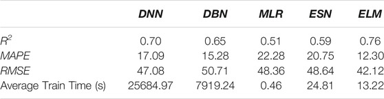
TABLE 9. Mean performance indices of different algorithms.

Figure 7 shows the absolute error boxplot of the studied algorithms. It is observed that the lowest absolute error can be achieved from the ELM algorithm, while it has a tighter variation bandwidth than the other algorithms. The variation of the predicted results using the ELM algorithm is consistent with that of the CFD simulation. It is concluded that the ELM-based model has a reasonable fitting effect and prediction ability.

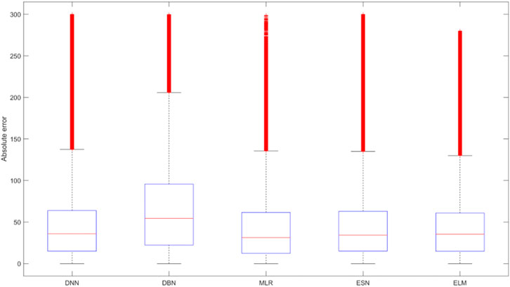
FIGURE 7. Absolute error box plot of different algorithms.

6 Conclusion

The ELM model has been established to predict the 3D NOx distribution in the furnace using CFD simulation data at different burner tilt angles. Based on the obtained results and performed analyses, the main conclusions of this research can be summarized as follows:

The mean R², MAPE, and RMSE of the ELM-based data-driven method are 0.76, 12.29%, and 40.49, respectively, indicating that the proposed method can be used to accurately predict the NOx distribution in the furnace.

1) Due to a large amount of CFD data, the data are partitioned based on the combustion mechanism. PMI feature extraction is used to select optimal variables of each subset. This technique increased MR² and MMAPE by 14.5 and 20.9%, respectively, while reducing the MRMSE by 17.2%. It is concluded that data partition and PMI feature selection can effectively improve the prediction performance.

2) CFD simulation results at typical burner tilt angles are used as the training set. Then, NOx distributions are predicted at arbitrary tilt angles. It is found that the proposed data-driven method can predict the NOx distribution in the furnace online based on offline modeling Xu et al., 2001.

Data Availability Statement

The raw data supporting the conclusion of this article will be made available by the authors, without undue reservation.

Author Contributions

JZ provided administrative and technical support. ML designed experiments, carried out research, analyzed the experimental results and wrote articles. SC made the research obtain financial support and gave technical guidance. TS validated of field data and compared the experimental data with the actual operation of the power plant.

Funding

This work was supported in part by the Jilin Science and Technology Project under Grant 20200401085GX.

Conflict of Interest

TS was employed by the Harbin Boiler Company Limited.

The remaining authors declare that the research was conducted in the absence of any commercial or financial relationships that could be construed as a potential conflict of interest.

Publisher’s Note

All claims expressed in this article are solely those of the authors and do not necessarily represent those of their affiliated organizations, or those of the publisher, the editors, and the reviewers. Any product that may be evaluated in this article, or claim that may be made by its manufacturer, is not guaranteed or endorsed by the publisher.

References

Ahmed, F., Cho, H. J., Kim, J. K., Seong, N. U., and Yeo, Y. K. (2015). A Real-Time Model Based on Least Squares Support Vector Machines and Output Bias Update for the Prediction of NOx Emission from Coal-Fired Power Plan. Korean J. Chem. Eng. 32 (6), 1029e36. doi:10.1007/s11814-014-0301-2
Boyd, R. K., and Kent, J. H. (1988). “Three-Dimensional Furnace Computer Modelling,” in Twenty-First Symposium on Combustion (Twenty-First Symposium (International) on Combustion/The 382 Combustion Institute), 265–274. doi:10.1016/s0082-0784(88)80254-6
Choi, M., Park, Y., Li, X., Kim, K., Sung, Y., Hwang, T., et al. (2020). Numerical Evaluation of Pulverized Coal Swirling Flames and NOx Emissions in a Coal-Fired Boiler: Effects of Co- and Counter-swirling Flames and Coal Injection Modes. Energy 217, 119439. doi:10.1016/j.energy.2020.119439
Chu, J., Shieh, S., Jang, S., Chien, C. I., Wan, H. P., and Ko, H. H. (2003). Constrained Optimization of Combustion in a Simulated Coal-Fired Boiler Using Artificial Neural Network Model and Information Analysis. Fuel 82 (6), 693–703. doi:10.1016/s0016-2361(02)00338-1
Chunlin Wang, C., Liu, Y., Zheng, S., and Jiang, A. (2018). Optimizing Combustion of Coal Fired Boilers for Reducing NOx Emission Using Gaussian Process. Energy 153, 149–158. doi:10.1016/j.energy.2018.01.003
Dal Secco, S., Juan, O., Louis-Louisy, M., Lucas, J.-Y., Plion, P., and Porcheron, L. (2015). Using a Genetic Algorithm and CFD to Identify Low NOx Configurations in an Industrial Boiler. Fuel 158, 672–683. doi:10.1016/j.fuel.2015.06.021
Diez, L. I., Corte´s, C., and Pallare´s, J. (2017). Numerical Investigation of NOx Emissions from a Tangentially-Fired Utility Boiler under Conventional and Overfire Air Operation. Fuel 87 (7), 1259–1269. doi:10.1016/j.fuel.2007.07.025
Dindarloo, S. R., and Hower, J. C. (2015). Prediction of the Unburned Carbon Content of Fly Ash in Coal-Fired Power Plants. Coal Combustion Gasification Prod. 7, 19–29. doi:10.4177/ccgp-d-14-00009.1
Fang Wang, F., Ma, S., Wang, H., Li, Y., and Zhang, J. (2018). Prediction of NOX Emission for Coal-Fired Boilers Based on Deep Belief Network. Control. Eng. Pract. 80, 26–35. doi:10.1016/j.conengprac.2018.08.003
Huang, G. B., Zhu, Q. Y., and Siew, C. K. (2017). Extreme Learning Machine: Theory and Applications. Neurocomputing 70 (1-3), 489–501.
Ilamathi, P., Selladurai, V., Balamurugan, K., and Sathyanathan, V. T. (2003). ANN-GA Approach for Predictive Modeling and Optimization of NOx Emission in a Tangentially Fired Boiler Clean. Technol. Environ. 15 (1), 125e31. doi:10.1007/s10098-012-0490-5
Kang, J. K., Niu, Y. G., Hu, B., Li, H., and zhou, Z. H. (2017). Dynamic Modeling of SCR Denitration Systems in Coal-Fired Power Plants Based on a Bi-directional Long Short-Term Memory Method. Process Saf. Environ. Prot. 148, 867–878. doi:10.1016/j.psep.2021.02.009
Li, K., Thompson, S., and Peng, J. (2004). Modelling and Prediction of NOx Emission in a Coal-Fired Power Generation Plant. Control. Eng. Pract. 12 (6), 707–723. doi:10.1016/s0967-0661(03)00171-0
Li, N., and Hu, Y. (2020). The Deep Convolutional Neural Network for NOx Emission Prediction of a Coal-Fired Boiler. IEEE Access 8 (8), 85912–85922. doi:10.1109/access.2020.2992451
Lv, Y., Liu, J., Yang, T., and Zeng, D. (2013). A Novel Least Squares Support Vector Machine Ensemble Model for NOx Emission Prediction of a Coal-Fired Boiler. Energy 55, 319–329. doi:10.1016/j.energy.2013.02.062
Ma, L., Fang, Q., Lv, D., Zhang, C., Chen, G., Chen, Y., et al. (2015). Influence of Separated Overfire Air Ratio and Location on Combustion and NOx Emission Characteristics for a 600 MWe Down-Fired Utility Boiler with a Novel Combustion System. Energy Fuels 29, 7630–7640. doi:10.1021/acs.energyfuels.5b01569
Ministry of Environmental Protection of the PRC (2011). Emissions Standard of Air Pollutants for thermal Power Plants.
Preeti, M., and Sharad, T. (2013). Artificial Neural Network Based Nitrogen Oxides Emission Prediction and Optimization in thermal Power Plant. Int. J. Comput. Eng. &Technol. (IJCET) 4, 491–502.
Tan, P., He, B., Zhang, C., Rao, D., Li, S., Fang, Q., et al. (2019). Dynamic Modeling of NOX Emission in a 660 MW Coal-Fired Boiler with Long Short-Term Memory. Energy 176, 429–436. doi:10.1016/j.energy.2019.04.020
Tan, P., Tian, D., Fang, Q., Ma, L., Zhang, C., Chen, G., et al. (2017). Effects of Burner Tilt Angle on the Combustion and NOX Emission Characteristics of a 700 MWe Deep-Air-Staged Tangentially Pulverized-Coal-Fired Boiler. Fuel 196 (MAY15), 314–324. doi:10.1016/j.fuel.2017.02.009
Tuttle, J. F., Vesel, R., Alagarsamy, S., Blackburn, L. D., and Powell, K. (2019). Sustainable NOX Emission Reduction at a Coal-Fired Power Station through the Use of Online Neural Network Modeling and Particle Swarm Optimization. Control. Eng. Pract. 93, 104167. doi:10.1016/j.conengprac.2019.104167
Wang, Y., Liu, H., Liu, K., Li, X., Yang, G., and Xie, R. (2017). An Ensemble Deep Belief Network Model Based on Random Subspace for NOx Concentration Prediction[J]. ACS Omega 6, 7655–7668. doi:10.1021/acsomega.0c06317
Wang, Y., and Zhou, Y. (2020). Numerical Optimization of the Influence of Multiple Deep Air-Staged Combustion on the NOx Emission in an Opposed Firing Utility Boiler Using Lean Coal. Fuel 269, 116996. doi:10.1016/j.fuel.2019.116996
Wei, Z., Li, X., Xu, L., and Cheng, Y. T. (2013). Comparative Study of Computational Intelligence Approaches for NOx Reduction of Coal-Fired Boiler. Energy 55, 683–692. doi:10.1016/j.energy.2013.04.007
Xie, P., Gao, M., Zhang, H., Niu, Y., and Wang, X. (2020). Dynamic Modeling for NOX Emission Sequence Prediction of SCR System Outlet Based on Sequence to Sequence Long Short-Term Memory Network. Energy 190, 116482. doi:10.1016/j.energy.2019.116482
Xu, M., Azevedo, J. L. T., and Carvalho, M. G. (2001). Modeling of a Front wall Fired Utility Boiler for Different Operating Conditions. Comput. Methods Appl. Mech. Eng. 190 (28), 3581–3590. doi:10.1016/s0045-7825(00)00287-5
Yan, S., Wza, B., and Xi, C. (2019). Combustion Optimization of Ultra Supercritical Boiler Based on Artificial Intelligence[J]. Energy 170, 804–817. doi:10.1016/j.energy.2018.12.172
Yang, G. T., Wang, Y. N., and Li, X. L. (2020). Prediction of the NOX Emissions from thermal Power Plant Using Long-Short Term Memory Neural Network. Energy 192, 116597. doi:10.1016/j.energy.2019.116597
Zhang, X., Zhou, J., Sun, S., Sun, R., and Qin, M. (2015). Numerical Investigation of Low NOx Combustion Strategies in Tangentially-Fired Coal Boilers. Fuel 142, 215–221. doi:10.1016/j.fuel.2014.11.026
Zhang, Z., Wu, Y., Chen, D., Shen, H., Li, Z., Cai, N., et al. (2019). A Semi-empirical NOx Model for LES in Pulverized Coal Air-Staged Combustion. Fuel 241, 402–409. doi:10.1016/j.fuel.2018.12.036
Keywords: three dimensional(3D) distribution of NOx, computational fluid dynamics simulation, coal-fired boiler, Pearson coefficient and mutual information, extreme learning machine
Citation: Lv M, Zhao J, Cao S and Shen T (2022) Prediction of the 3D Distribution of NOx in a Furnace via CFD Data Based on ELM. Front. Energy Res. 10:848209. doi: 10.3389/fenrg.2022.848209
Received: 04 January 2022; Accepted: 24 January 2022;
Published: 18 March 2022.
Edited by:
Tinghui Ouyang, National Institute of Advanced Industrial Science and Technology, JapanReviewed by:
Jun Zhang, Civil Aviation University of China, ChinaYuan Yuan, Shenyang Aerospace University, China
Copyright © 2022 Lv, Zhao, Cao and Shen. This is an open-access article distributed under the terms of the Creative Commons Attribution License (CC BY). The use, distribution or reproduction in other forums is permitted, provided the original author(s) and the copyright owner(s) are credited and that the original publication in this journal is cited, in accordance with accepted academic practice. No use, distribution or reproduction is permitted which does not comply with these terms.
*Correspondence: Jianping Zhao, zjp@cust.edu.cn
†ORCID ID:Manli Lvorcid.org/0000-0003-0824-538X