Bypass diode effect and photovoltaic parameter estimation under partial shading using a hill climbing neural network algorithm

1 Introduction

The importance of using renewable energy has never been so debated worldwide as it is today. National governments, companies and citizens are increasingly concentrating efforts to accelerate the energy transition towards a sustainable and environmentally friendly energy consumption model. Among the different sources of renewable energy, photovoltaic (PV) energy has been one of the most relevant in terms of electricity production. In recent years, new developments in the PV sector have contributed to increasing the efficiency of this energy production technology, as well as in reducing its cost. However, it is hoped that continued advances will enable researchers and manufacturers to achieve even more efficient and less expensive PV energy production systems, allowing greater penetration of this energy production technology. In addition, PV energy has been combined in several strategies for the use and transformation of essential resources, such as in water desalination (Manokar et al., 2018) and in the use of sunlight on building facades (Karthick et al., 2020), allowing to effectively explore the resources and reduce costs.

The number of installed PV plants has been increasing considerably and floating PV has been a good alternative for several investors in the energy sector (REN21, 2021). However, predicting PV energy production remains a complex task due to the variability and unpredictability of solar radiation. To answer this problem, researchers have been continuously developing new models and forecasting methods, but the operation of real-time PV systems can still be improved, particularly under partial shading conditions (PSC).

In the literature, there are numerous approaches of greater or lesser complexity to deal with PSC, the main purpose being to mitigate power loss. To maximize the output power under PSC, the bypass diodes are activated as a function of the photoelectric current I_ph of a given PV cell or array. For example, Bai et al., (2015) used the single-diode model (SDM) to simulate the current-voltage (I-V) characteristics under uniform and non-uniform irradiances (with shading). To more accurately predict the performance of a PV system with PSC, Ishaque et al., (2011) used the double-diode model (DDM) because it is more accurate for lower irradiance levels. This model allows the simulation of maximum power point tracking (MPPT) algorithms and electronic power converters. Alternatively, Batzelis et al., (2014) used the SDM based on the Lambert W function (LWF) to evaluate the performance of strings of PV modules under PSC in order to make SDM explicit. This model expresses the PV string voltage as an explicit function of the current, avoiding an iterative procedure, with the bypass diode described by a logarithmic equation. In turn, Wang and Hsu, (2011) used the Newton-Raphson method (NRM) to estimate the I-V characteristic curve of five different connection configurations (simple series, series-parallel, total-cross-tied, bridge-linked and honeycomb) of PV cells with different types and levels of partial shading, as this is an effective method to approximate the non-linear equation roots of the model. Using the same connection configurations, Bingöl and Özkaya, (2018) analyzed partial shading in a PV array in six different scenarios, while Zhu et al., (2019) analyzed the effect of partial shadow on the photoelectric current I_ph and series resistance R_s. In contrast, Moreira et al., (2021) represented the behavior of PV systems under PSC through an improved model with a superposition technique that considers the voltage drop caused by the bypass diodes. Kermadi et al., (2020) proposed an analytical approach to predict I-V characteristics under PSC that uses the DDM and requires only the information in the standard test condition (STC), while Zhang et al., (2021) developed an explicit analytical model based on SDM for PSC that requires lower computational cost when compared to NRM and FWL.

To mitigate power loss and prevent hot spots when a PV system is shaded, a common strategy is to bypass the shaded cells or modules using bypass diodes. However, this strategy leads to the appearance of multiple peaks in the characteristic curve and the need for robust MPPT algorithms capable of tracking the highest power peak. Alqaisi and Mahmoud, (2019) developed a model that uses overlapping bypass diodes to evaluate the performance of a PV module in terms of electrical characteristics, hot-spot formation and quantification of power loss. Mohammed et al., (2020) studied the temperature distribution in a shaded PV module when the bypass diode’s state changes from inactive to active and concluded that thin edge shadows can lead shaded cells to very high temperatures when the bypass diode is inactive, and that this state change is more effective with larger shadows. Lee et al., (2021) analyzed the electrical and thermal characteristics of a PV array with mismatch between strings due to a short-circuit failure of bypass diodes, verifying that in this situation, in addition to heating the PV cells, the bypass diode can reach high temperatures leading to its deformation and even cause accidents like fire.

Predicting the I-V characteristics of a PV system under uniform irradiance is a complex task due to the inherent implicit nature in estimating the PV parameters of the model under consideration. However, PSC (non-uniform irradiance) still creates an added difficulty due to the presence of multiple power peaks in the characteristic curve. This makes it even more important to use accurate and efficient methods for estimating the PV parameters. As an alternative to efficient but sometimes inaccurate analytical methods, metaheuristic methods have assumed great relevance in the literature regarding the estimation of PV parameters. These include the Runge-Kutta optimizer (RUN) (Shaban et al., 2021), grouped beetle antennae search (GBAS) (Sun et al., 2021), neural network algorithm with reinforcement learning (RLNNA) (Zhang, 2021) and enhanced adaptive butterfly optimization algorithm (EABOA) (Long et al., 2021). Concretely, metaheuristic methods have the advantage of considering all sample points of the I-V curve, thus leading to more accurate and reliable solutions. In addition, they are suitable for solving complex and multimodal problems due to a global search capability, computational simplicity and easy implementation. However, to avoid premature convergence, metaheuristic methods must strike a good balance between intensification and diversification mechanisms. Moreover, less efficient search mechanisms can lead to the need for large populations requiring high computational costs. Also, most of these methods are highly dependent on the proper adjustment of control parameters. Abdel-Basset et al., (2021) proposed a modified artificial jellyfish search optimizer (MJSO) with a strategy to mitigate premature convergence, which requires adjustment of several control parameters. To minimize the probability of the Harris hawks optimization (HHO) getting stuck in local optima, Naeijian et al., (2021) added a strategy that eliminates the worst solutions and generates new solutions in the search space. However, the improved algorithm, whippy HHO (WHHO), requires two new control parameters. Yesilbudak et al., (2021) used a grey wolf optimizer with a dimension learning-based hunting search strategy (I-GWO) to mitigate the imbalance between intensification and diversification mechanisms and the lack of population diversity. To improve the global search capability of teaching-learning-based optimization (TLBO) and avoid local minima, Mi et al., (2021) proposed an adaptive TLBO with experience learning (ELATLBO). The modification consisted of dividing the population into two parts (best and worst agents) according to the objective function, where the best agents are used in local search and the worst in global search. Sallam et al., (2021) proposed an improved gaining-sharing knowledge (IGSK) algorithm that minimizes the dependence of several control parameters. Specifically, a mechanism was introduced that automatically adjusts the knowledge rate responsible for ensuring a good balance between agents with greater and lesser knowledge. To take advantage of intensification and diversification mechanisms with different capabilities, several metaheuristics have been combined in the literature (hybrid methods) and applied to the PV parameter estimation, such as the hybrid marine predators-slime mould algorithm (HMPA) (Yousri et al., 2021), enhanced marine predators algorithm (EMPA) (Abd Elaziz et al., 2021) and Laplace’s cross search mechanism combined with Nelder-Mead simplex (LCNMSE) (Weng et al., 2021). However, the hybrid methods require the adjustment of a greater number of control parameters and larger populations to enhance the different search mechanisms, leading to high computational cost.

Recently, other approaches to deal with the PV parameter estimation problem have been proposed in the literature. Nunes et al., (2020) proposed a multiswarm spiral leader particle swarm optimization (M-SLPSO) algorithm that, unlike most metaheuristics, has several swarms guided by different leaders, maintaining a diversity of exploratory trajectories when building new solutions during the search process and mitigating population stagnation. To increase reliability when accurately estimating PV parameters with metaheuristics, Li et al., (2021) proposed a data prediction-based metaheuristic algorithm (DPMhA) that extends the measured I-V data via extreme learning machine-based data prediction. In response to emerging PV technologies, Nunes et al., (2021) proposed a mathematical model that determines the optimal number of diodes in the equivalent electrical circuit for each technology by using a guaranteed convergence particle swarm optimization (GCPSO) metaheuristic algorithm.

Despite the efforts of many researchers to estimate PV parameters with accuracy, reliability and low computational cost, there is still need of new approaches, namely for the operation of PV systems in real-time and under PSC. To fill this gap and overcome some of the drawbacks associated with metaheuristic methods in estimating PV parameters, we propose a new method that uses an improved metaheuristic to ensure a good balance between the intensification and diversification mechanisms, without any adjustment of control parameters. Specifically, we studied the bypass diode effect on the I-V characteristic curve and quantified the power loss under PSC. The possible presence of hot spots was also considered through thermographic analysis of the temperature distribution. Furthermore, a hill climbing neural network algorithm (HCNNA) was proposed to estimate the PV parameters of SDM and DDM with and without partial shading. The effect of bypass diodes was studied in an outdoor experimental environment by creating two shading scenarios with different patterns. To validate the HCNNA, we used standard literature datasets under uniform irradiance and experimentally measured datasets with shading. The results are promising and show that HCNNA has an extremely competitive performance in the PV parameter estimation problem.

The main contributions of this paper are as follows:

1) Monitoring PV power losses and the presence of hot spots under partial shading.

2) A novel HCNNA method for PV parameter estimation with and without partial shading.

3) The proposed HCNNA establishes a good balance between diversification and intensification mechanisms and does not use any control parameters.

4) HCNNA has an adaptive movement strategy to prevent population stagnation and premature convergence.

5) HCNNA performance was extensively investigated by applying several experimental datasets, and the results demonstrate high accuracy and reliability.

The paper is structured as follows: Section 2 reviews the PV models used and formulates the PV parameter estimation problem; Section 3 presents background and methods for PV parameter estimation and describes the proposed HCNNA; Section 4 analyzes the bypass diode effect in PV modules; Section 5 tests the HCNNA performance in estimating PV parameters; Section 6 concludes the paper.

2 PV modelling

Describing the non-linear characteristics of a PV cell or module is essential to estimate the power generated by a PV system under real operating conditions. For this purpose, two mathematical models are adopted in the literature, the single-diode model (SDM) and the double-diode model (DDM).

2.1 Single-diode model

The SDM, Figure 1A formed by: a current source that represents the photoelectric current (I_ph) generated by solar radiation; a parallel connected diode to describe the physical effects at the PN junction; a series resistance (R_s) considering the ohmic losses; and a parallel resistance (R_p) considering the leakage currents.

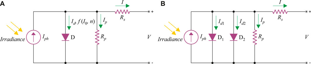
FIGURE 1. Equivalent circuit: (A) single-diode model; (B) double-diode model.

Considering Shockley’s equation and according to Kirchhoff’s laws, the output current (I) is obtained by Eq. 1.

where I₀ is the reverse saturation current of the diode, V is the output voltage, n is the diode ideality factor, and V_t is the thermal voltage obtained by Eq. 2.

where k is the Boltzmann constant (1.3806503 × 10⁻²³ J/K), q is the electron charge (1.60217646 × 10⁻¹⁹ C), T is the cell temperature (K), and N_s is the number of cells connected in series.

2.2 Double-diode model

The DDM, in Figure 1B, is used to more accurately estimate the PV power generated under real operating conditions, namely under low irradiance levels. This model has a second diode in parallel with the current source to better describe the physical effects at the PN junction. In particular, the first diode represents the diffusion current at the PN junction, while the second diode represents the recombination effects in the semiconductor. From a computational point of view, DDM is less advantageous due to the greater number of parameters.

Considering Shockley’s equation and according to Kirchhoff’s laws, the output current (I) for the DDM is obtained by Eq. 3.

where n₁ and n₂ are the ideality factors of diodes D₁ and D₂, and I₀₁ and I₀₂ are the reverse saturation currents of diodes D₁ and D₂, respectively.

2.3 Photovoltaic models on partial shading condition

A common problem in the operation of PV systems, under real conditions, is the probability of occasional periods when the irradiance level is non-uniform. This problem is called the partial shading condition (PSC) and considerably affects the power generated due to the voltage drop in the shaded PV cells. Some common causes for PV cells not receiving solar irradiance uniformly include dirt on the surface, the presence of obstacles around cells causing temporary shadows throughout the day, and the presence of clouds in the sky. Under such conditions, the PV cells or modules area is partially shaded, leading to the occurrence of potential divergences in the generated current, which in turn can cause hot spots, compromising the proper functioning of the PV system. Briefly, the shaded cells start to dissipate electrical energy in the form of heat due to the inversion in polarity as a result of potential divergences between the cells connected in series.

To overcome this problem, which can lead to significant losses of generated PV power and even damage the PV modules, the most common practice is to install bypass diodes (D_by), in antiparallel with the PV module cells, aiming to bypass the current of the reverse polarized cells. Normally, the PV module cells are grouped in m groups according to the number of bypass diodes adopted by the manufacturer. Thus, it is possible to take one or more groups of PV cells out of operation, while the remaining continue to operate without any disturbance. Figure 2 shows the equivalent electrical circuit for the SDM and DDM of a PV module with m bypass diodes.

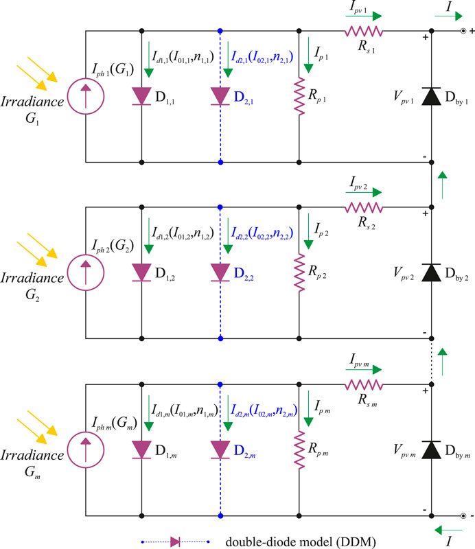
FIGURE 2. Equivalent circuit for the SDM and DDM under partial shading conditions.

The bypass diodes connected in antiparallel are Schottky diodes. Schottky diodes offer a very low forward voltage drop, typically less than 0.4 V (Liu et al., 2021), high current density, fast reverse recovery time, low resistance and therefore can be modeled as a resistance (R_by) that depends on the photoelectric current, I_ph. According to Seyedmahmoudian et al., (2013) in a reversed-polarity, the bypass diode is represented as a high resistance (10¹⁰ Ω), while in a direct-polarity it is represented as a low resistance (10⁻² Ω), as stated in Eq. 4.

Therefore, to mitigate the PV power loss under PSC and obtain the respective output current and voltage, Eqs 5, 6 are considered (Seyedmahmoudian et al., 2013).

where I_pv and V_pv are the output current and voltage of each group of PV cells, respectively; G is the irradiance with G₁ > G₂ > G_m; and u represents the number of diodes in the equivalent circuit of PV model with u = 1 for SDM and u = 2 for DDM.

2.4 Problem formulation

Estimating the I-V characteristics of a PV system through metaheuristic methods requires the definition of an objective function that evaluates the error between experimental and estimated data. Several performance indexes can be used for this purpose, such as: the sum squared error (SSE), mean square error (MSE), root mean square error (RMSE), absolute error (AE), and mean absolute error (MAE) (Laudani et al., 2014). The selected objective function was the RMSE, expressed by Eq. 7, as it is a common performance index in the literature on PV parameter estimation (Mi et al., 2021).

where N represents the experimentally measured set of points (I_z,V_z), with z ε N, and Î(V_z,τ) represents the estimated value of the current as a function of the unknown parameters τ that characterize the PV models.

To solve the equivalent equation of the PV models under consideration, i.e., estimate the current values of the characteristic curve, the Newton-Raphson method (NRM) was used with a threshold value of 10^-10. NRM was chosen because it is simple and fast in approximating the roots of any non-linear equations. Furthermore, for a fair comparison with the literature, the unknown parameters were limited according to Table 1.

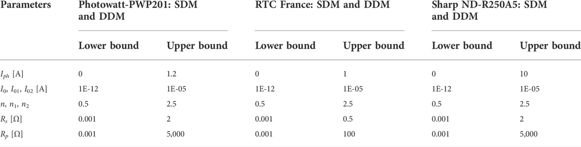
TABLE 1. Parameter ranges for the PV models in each case study.

3 Background and methods

In the specialized literature, there are several methods to estimate PV parameters, which differ in complexity, computational cost, convergence rate, accuracy and popularity. However, in recent years, there has been a clear trend towards the use of metaheuristic methods as they are extremely efficient in solving non-convex and multimodal optimization problems (Cotfas et al., 2021). This trend is mainly due to their search mechanisms, i.e., the intensification and diversification mechanisms. The intensification mechanism (local search) attempts to build new solutions in regions of the search space that have already been explored, i.e., in regions where high-quality solutions have already been found. Meanwhile, the diversification mechanism tries to build solutions in unexplored regions of the search space, i.e., in regions that differ significantly from the best solutions found so far. However, the efficiency of these methods depends, profoundly, on the balance between the different techniques inherent to their diversification and intensification mechanisms and on the correct adjustment of their control parameters. The hill climbing neural network algorithm (HCNNA) overcomes these constraints, as it does not require the adjustment of any control parameter and combines several intensification and diversification mechanisms to achieve high-quality solutions with low computational cost. Furthermore, HCNNA has been combined with NRM to overcome the implicit and non-linear nature inherent in the mathematical equations that characterize the PV models.

3.1 Neural network algorithm

The neural network algorithm (NNA) (Sadollah et al., 2018) is a metaheuristic optimization algorithm inspired by artificial neural networks (ANN) and by the biological functioning of the human nervous system. ANNs are composed of several neurons, interconnected and distributed through different layers, capable of receiving, processing, transforming and sending information. Through a learning process, ANNs present a computational structure capable of performing interpolations and extrapolations between the input and output pairs provided, adjusting the weights associated with the existing connections between neurons. To mimic this process, NNA is an optimization algorithm without control parameters, i.e., its performance and reliability does not depend on the adjustment of any control parameters to achieve high-quality solutions. Like any other metaheuristic algorithm, NNA starts with an initial population (with size n_pop × d) randomly generated within the multidimensional search space, where n_pop is the number of agents in the population and d is the number of dimensions of the optimization problem. In the initial population (X), expressed by Eq. 8, x represents the positions of each agent (designated of pattern solution), and the initial population is composed of several pattern solutions.

However, in addition to the initial population, it is also necessary to initialize a weight matrix (W) that mimics the interconnections between neurons, expressed by Eq. 9, with dimension n_pop × n_pop and random values between 0 and 1.

To avoid NNA premature convergence due to the weights showing an increasing tendency in a specific direction (values greater than 1), the sum of the weights cannot exceed unity. This condition can be defined mathematically through the Eqs 10, 11.

At each iteration, the new positions of pattern solutions are calculated using Eqs 12, 13 and later evaluated using the objective function.

Once the new pattern solutions are determined, the weight matrix must also be updated based on the best weight value found so far (${\overrightarrow{W}}_{Target}$). The weight matrix is updated through Eq. 14, considering the conditions described in Eqs 10, 11.

NNA presents two different strategies to avoid premature convergence and population stagnation: the bias operator and transfer function operator. The bias operator, at an initial stage, favors the diversification mechanism by modifying, at each iteration, a percentage of each pattern solution (x) in the population of pattern solutions (X) and the weight matrix (W). For this, at the beginning of the optimization process, the bias value (β) is initialized to one and decremented as iterations (t) progresses, through the Eq. 15.

The transfer function operator favors the intensification mechanism, forcing the creation of new agents (${\overrightarrow{X}}_i$) around the best solution found so far (${\overrightarrow{X}}_{Target}$), according to Eq. 16.

The balance and harmony between the diversification mechanism (bias operator) and intensification mechanism (transfer function operator) is controlled by a probability. This probability depends on the bias value (β) and a random number (p) with a uniform distribution between 0 and 1.

3.2 Hill climbing

Hill climbing (HC) is an elitist optimization algorithm that favors the intensification mechanism, i.e., a local search, by exploring its neighborhood (Alweshah et al., 2020; Jately et al., 2021). Starting from an initial solution $\overrightarrow{x}=(x_1,x_2\dots x_d)$, at each iteration the HC algorithm tries to advance to a better solution $\overrightarrow{x^{\prime }}=(x_1^{\prime },x_2^{\prime }\dots x_d^{\prime })$, through two operators: N-operator and S-operator. The N-operator is used to build new solutions, in a certain neighborhood, through a movement strategy, as represented by Eq. 17.

where $\overrightarrow{b{w}_i}$ is the distance bandwidth between the current and neighboring solution and n_b is the number of neighbors. This movement strategy can be deterministic or stochastic and must be updated, at each iteration, to achieve a higher convergence rate and HC efficiency. The S-operator is responsible for evaluating the solution or neighboring solutions through the objective function. If the neighboring solution performs better than the current solution, i.e., $f\left(\overrightarrow{x_i^{\prime }}\left(t\right)\right)<f(\overrightarrow{x}\left(t\right))$, the current solution $\overrightarrow{x}$ will be replaced by the new solution $\overrightarrow{x_i^{\prime }}$. HC execution ends when a certain stopping criterion is reached, such as when, after a certain number of iterations, none of the neighboring solutions improve the current solution or when the maximum number of predefined iterations is reached.

3.3 Hill climbing neural network algorithm

In this section, we present the hill climbing neural network algorithm (HCNNA) in detail, which aims to improve NNA performance. Figure 3 presents the HCNNA flowchart. First, all variables inherent to the optimization problem and the proposed method are initialized, such as: the problem dimension (d), lower and upper bounds, number of agents (pattern solutions) of the population (n_pop), bias value (β), maximum number of iterations (t_max). Then, the HCNNA performs the initial positioning of the weight matrix (W) and pattern solutions (X). An initial random positioning was performed, within the multidimensional search space, considering a population of 15 agents per dimension and a maximum number of 150 iterations per dimension. At each iteration, the movement of each pattern solution is performed as described above and detailed in Eqs 12, 13. However, to ensure greater diversification and randomness in updating the weight matrix (W), the logistic chaotic map was introduced in Eq. 14. Chaotic maps result from chaos theory and are based on deterministic differential equations that exhibit extremely random (chaotic) behavior. The logistic chaotic map with a = 4, initialized with a value of 0.7, as suggested in the literature, is expressed by Eq. 18.

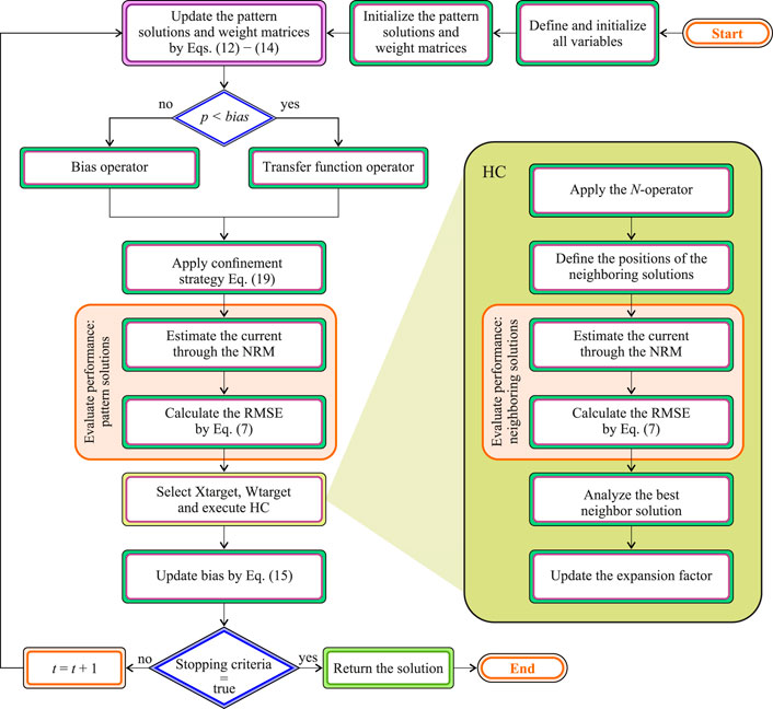
FIGURE 3. Flowchart of the proposed HCNNA.

Subsequently, the bias value (β) is compared with a random number (p) from a uniform distribution between 0 and 1. This comparison triggers the two strategies inherent to the NNA to avoid premature convergence and population stagnation, namely the bias operator and transfer function operator. In addition, and as part of the transfer function operator strategy, the logistic chaotic map (Eq. 18) was used to achieve greater diversification in the built of new pattern solutions.

The confinement strategy given by Eq. 19 was implemented to prevent new positioning of pattern solutions outside the multidimensional search space, during successive iterations.

In this strategy, if the lower bound (lb) or upper bound (ub) are exceeded, the agent’s movement is modified, ensuring that the new positioning is within the search space (according to Table 1). Once confinement is verified, for each pattern solution of the population, the estimated current ${\widehat{I}}_{(V_z,\text{τ})}$ is obtained through the NRM with a stop criterion of 10^-10, for each set of points (I_z,V_z) measured experimentally. Its performance is evaluated through the objective function defined above, which consists of the RMSE between the measured and estimated data, expressed by Eq. 7.

Then, the best global performance of all pattern solutions of the population so far (${\overrightarrow{X}}_{Target}$) and, consequently, the best value of weights found so far (${\overrightarrow{W}}_{Target}$) are determined. Based on the information acquired by the NNA, at each iteration, the HC algorithm tries to explore the neighborhood of the ${\overrightarrow{X}}_{Target}$ through a movement strategy defined by the N-operator. This movement strategy consists of the construction of 2d neighbor solutions defined by a neighborhood given by Eq. 20.

where ${\overrightarrow{X}}_{Target}\left(t\right)$ is the position of the best pattern solution in the current iteration, ${\overrightarrow{X}}_{Target}\left(t-1\right)$ is the previous position of the best pattern solution and $\overrightarrow{\delta }\left(t\right)$ is an expansion factor that controls the diameter of the neighborhood. However, if any component of $\overrightarrow{bw}$ (dimension) is null, the position of the best pattern solution so far is assigned to that component, weighted by a scale factor (0.1), i.e., $0.1 {\overrightarrow{X}}_{Target}\left(t\right)$. Once the neighborhood region is established, the neighboring solutions are selectively positioned at their vertices, using Eq. 17, and evaluated through the established objective function (S-operator). If any neighboring solution presents a better performance than the current best solution (${\overrightarrow{X}}_{Target}\left(t\right)$), this information is transmitted to the NNA and analyzed to identify the several components (dimensions) that contributed to this improvement in the objective function. This analysis is essential to control the dilation factor: if there is an improvement in the objective function, the diameter of the neighborhood of this component is dilated (doubled) in the next iteration. Otherwise, the expansion factor value is reset to the unit value. The execution of the HCNNA ends when the established stop criterion is reached, namely the maximum number of allowed iterations (150 iterations per dimension).

4 Analysis of bypass diodes effect

As mentioned in Section 2.3, the bypass diodes present in the PV modules have the function of bypassing the electrical current from the cell groups where potential divergences occur, as shown in Figure 4. These potential divergences can originate from mismatch losses (manufacturing defects or different technical characteristics; incorrect installation, interconnection failures and possible damage) or shading losses (partial shading).

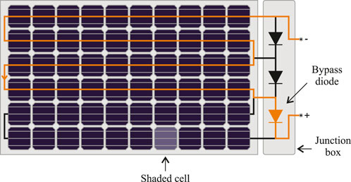
FIGURE 4. Shaded PV module with one bypass diode activated.

This section studies the effect of bypass diodes on the I-V and P-V characteristic curves in order to mitigate power losses under PSC. Temperature variation of the shaded cells was also analyzed to show the formation of hot spots and possible consequences. Therefore, to study the impact of PSC on PV power generation and the effect triggered by the direct polarization of bypass diodes, two partial shading scenarios were considered, which included several shading patterns measured experimentally through the Itech DC electronic load IT8512A+. For this, a Sharp ND-R250A5 PV module (Sharp, 2012) with 60 polycrystalline silicon cells connected in series was used. Cells were divided into three strings, each protected with a bypass diode, i.e., the PV module for every 20 cells included a bypass diode. The irradiance and temperature data for each of the shading patterns were obtained with the solar irradiance sensor Ingenieurbüro Si-13TC-T. Temperature variation of the shaded cells was measured with an infrared thermographic camera Flir i7. All thermographic images were taken with the camera’s emissivity of 0.95.

The first scenario consisted of shading only one cell of the PV module with different shaded areas (0%, 20%, 40%, 60%, 80% and 100%), for a total of six shading patterns (pattern 1 to pattern 6) as shown in Figure 5A. The second scenario consisted of gradually shading one or more 20-cell strings of the PV module (each with a bypass diode), as shown in Figure 5B. Pattern A consisted of shading only one string, pattern B consisted of shading two strings, and pattern C consisted of shading all three strings.

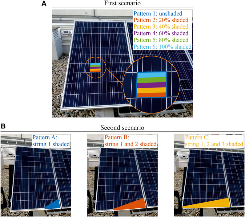
FIGURE 5. Shading scenarios with Sharp ND-R250A5 PV module: (A) just a shaded cell; (B) different shaded strings.

The irradiance and temperature values corresponding to each of the experimentally measured shading patterns were as follows: Pattern 1 962 W/m² at 52°C; Pattern 2 1,005 W/m² at 54°C; Pattern 3 1,006 W/m² at 55°C; Pattern 4 1,013 W/m² at 56°C; Pattern 5 1,023 W/m² at 56°C; Pattern 6 1,007 W/m² at 56°C; Pattern A 881 W/m² at 48°C; Pattern B 955 W/m² at 52°C; and Pattern C 965 W/m² at 52°C.

4.1 Effect of bypass diodes on characteristic curves

The partial shading of a PV cell or module drastically reduces the output current since this is directly proportional to the incident irradiance; and, as explained previously, this leads to operation in reverse polarity. Since the use of bypass diodes is common practice to mitigate the constraints caused by shading, it is important to understand their effects on the characteristic curves and, consequently, on the real-time maximum power extraction.

In the first shading scenario, with gradually shading of only one PV cell of the module used (connected in series in a string of 20 cells protected by a bypass diode), the direct polarization of the respective bypass diode depended on the shaded area, as shown in Figures 6A,B. As the shaded area increases, the bypass diode is directly polarized at lower current levels, causing a voltage drop (equivalent to the sum of the 20 cells of the respective string) and consequently a significant decrease in output power. The power curves (P-V) also indicate that direct polarization of the bypass diode leads to an additional power peak, making it difficult to track the maximum power, mainly when the cell is shaded around 60%, as both peaks are close to the same value.

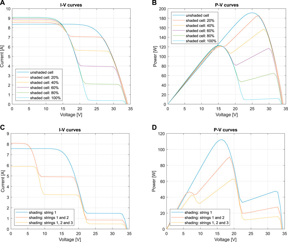
FIGURE 6. Effect of bypass diode with Sharp ND-R250A5 PV module: (A) I-V curves for first scenario; (B) P-V curves for first scenario; (C) I-V curves for second scenario; (D) P-V curves for second scenario.

Specifically, for pattern 1 (962 W/m² of irradiance), in which the characteristic curve was obtained without shading, the maximum power point (MPP) was 191.26 W. Patterns 2, 3, 4, 5 and 6, with shading, comprised a similar irradiance, since measurements were carried out in an outdoor environment between 1005 W/m² and 1023 W/m². The MPP value for these patterns was 185.14, 157.18, 122.48, 122.62 and 123.05 W, respectively. Although pattern 1 was measured with slightly lower irradiance, its power value (191.26 W) was used as a reference to quantify each shading pattern’s power loss. Thus, the power loss for pattern 2 was 3.2%, which corresponds to 6.12 W; pattern 3, 17.8% (34.08 W); pattern 4, 36.0% (68.78 W); pattern 5, 35.9% (68.64 W); and pattern 6, 35.7% (68.21 W). Patterns 4, 5 and 6 presented approximately the same power loss, as their peak with highest power corresponded to the peak with the lowest voltage, as guaranteed by the correct operation of the remaining module strings. Clearly, a single shaded cell in a PV module can lead to large losses, and it is extremely important to consider all the surrounding obstacles when sizing and installing systems; to carry out cleaning maintenance; and develop methods to effectively deal with shading caused mainly by clouds.

The second shading scenario analyzed the direct polarization of bypass diodes in different strings, shaded according to Figure 5B (patterns A, B and C). Initially, only one string from the PV module was shaded, later two strings were shaded and finally the three strings were shaded simultaneously. The I-V curves in Figure 6C reflect the direct polarization of the bypass diodes at different current levels, according to the shaded area in each string. The P-V curves in Figure 6D show the existence of a new power peak resulting from the direct polarization of another bypass diode.

Pattern A, measured under an irradiance of 881 W/m², recorded an MPP of 112.23 W; pattern B with 955 W/m² had an MPP of 90.30 W; while pattern C with 965 W/m² recorded only an MPP of 62.67 W. The maximum power, 191.26 W, measured without shading in the first scenario (under 962 W/m² of irradiance), was used as a reference for evaluating power loss in the second scenario: for pattern A was 41.3%, corresponding to 79.03 W; for pattern B, 52.8% (100.96 W); pattern C, 67.2% (equivalent to 128.59 W). Considering the maximum power of the module in the STC (250 W), the power loss (also affected by the temperature increase) was about 75% for pattern C, which shows the importance of real-time monitoring of the PV systems. Note that bypass diodes can be activated by PSC or string mismatch, drastically reducing the output power.

To reduce losses, ideally, each cell would have a bypass diode. However, from a constructive point of view, this is not feasible and would also make it difficult to track the MPP. To address this problem, in recent years, strategies to reconfigure connections between strings have been studied to maximize the output power in specific situations such as shading.

4.2 Temperature variation of the shaded cells

Reverse polarity operation resulting from partial shading or other divergences leads to the formation of hot spots that can damage PV cells or modules. Thus, during the experimental test, thermographic recording of the temperature distribution in the PV module was carried out in both shading scenarios with each of the patterns. To clearly analyze temperature evolution before the bypass diode switched to the active state, the respective I-V curves were traced for approximately 8 min.

Figure 7 shows the temperature distribution in the PV module for the first shading scenario. For pattern 1, with the characteristic curve traced under uniform irradiance, the figure shows slight heating (approximately 5°C) mainly in three cells, which resulted from insignificant divergences derived from their aging or principle of degradation. For patterns 2, 3, 4, 5 and 6, hot spots were observed in the shaded cell, independently of the shading percentage, whose temperature reached 87.9°C, 98.1°C, 96.3°C, 84.9°C and 67.4°C, for each pattern respectively. Temperature increased to higher values when the shaded percentage was around 50%, specifically with patterns 3 and 4. When the bypass diode went into the active state, the respective string was taken out of operation and the temperature immediately began to drop, becoming uniform with the other cells.

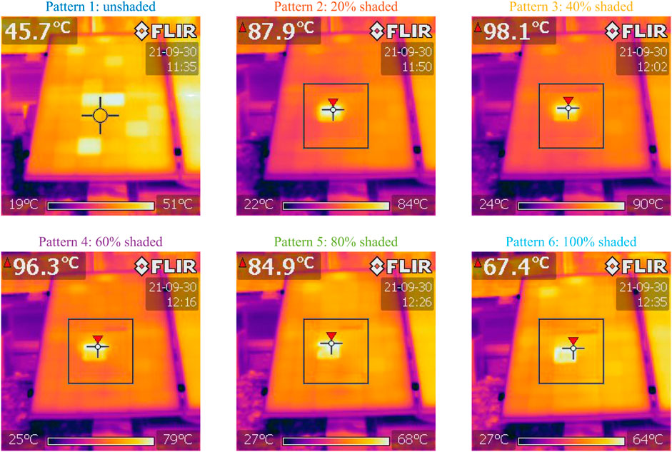
FIGURE 7. Temperature variation with a PV cell under partial shading (Sharp ND-R250A5 PV module: first scenario).

For the second shading scenario, the temperature distribution in the PV module is shown in Figure 8. In this case, two cells in each string were shaded with different proportions according to the shading pattern. By observing the temperature distribution (Figure 8), it is concluded that there was a significant increase only in the cell with greatest shaded area. Thus, for each string, an elevated temperature level was recorded in one of the shaded cells until the bypass diode went into the active state. Specifically, for pattern A, a temperature of 74.8°C was recorded, while patterns B and C recorded 72.2 and 75.3°C, respectively.

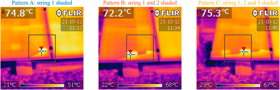
FIGURE 8. Temperature variation with different cell strings under partial shading (Sharp ND-R250A5 PV module: second scenario).

Regarding the temperature of the bypass diodes, there was an increase of about 5°C when they switched to the active state. However, Lee et al. (2021) showed that in case of failure, bypass diodes can reach very high temperatures capable of causing accidents.

5 Photovoltaic parameter estimation: Simulation and results

PV parameter estimation becomes more complex when the PV systems are under partial shading, as there are multiple power peaks due to the direct polarization of the bypass diodes. Thus, effectively determining accurate solutions for simulation models that consider mitigation of shadow effects in a PV system requires more robust I-V characteristics prediction methods, due to the need for real-time monitoring.

In this section, the proposed HCNNA was validated in PV parameter estimation using the RTC France cell and Photowatt-PWP201 module (both standard data in the literature) under uniform irradiance. Subsequently, the HCNNA was validated under partial shading using data measured experimentally with the Sharp ND-R250A5 PV module, presented previously in Section 4 (first and second shading scenarios). The validation considered the SDM and DDM, as they are the most used in the literature, and used the RMSE as a performance index.

HCNNA performance was compared with several recent metaheuristics in the literature, particularly with the original NNA, which was also implemented. To minimize statistical errors, 30 runs were performed with the different datasets. The population depended on the size of the optimization problem (15 agents per dimension), as well as the maximum number of iterations (150 iterations per dimension). All computational work was carried out in Matlab^® using a computer with an Intel^® Xeon^® E5-2630 v3 @2.40 GHz CPU processor, 64 GB RAM, and Windows 10 Professional 64-bit operating system.

5.1 Results with standard literature data

For the Photowatt-PWP201 PV module standard dataset, measured under 1000 W/m² irradiance and 45°C temperature (Easwarakhanthan et al., 1986), the PV parameter estimation results with SDM are presented and compared with the ones presented in literature, as shown in Table 2. The results displayed in this table show that the accuracy obtained by HCNNA was higher than the original NNA (0.43% better). Specifically, the HCNNA achieved an RMSE of 2.046535E-03, while the NNA obtained 2.055430E-03. The MJSO was closest to HCNNA, with an RMSE of 2.0530E-03. The remaining methods were less accurate (2.425E-03).

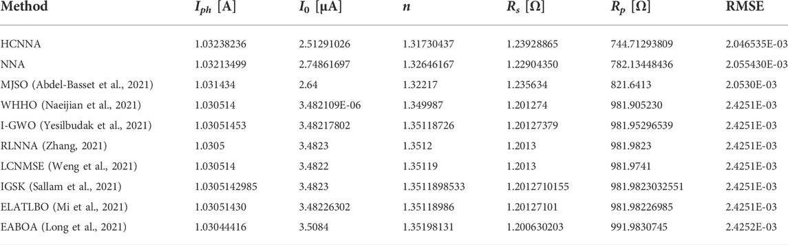
TABLE 2. Comparison of results between HCNNA and other state-of-the-art metaheuristics for the Photowatt-PWP201 PV module with SDM.

Table 3 Presents the results with DDM for the Photowatt-PWP201 PV module. In this case, WHHO obtained the best RMSE value (2.046534E-03). The HCNNA achieved an RMSE of 2.046535E-03, just as with the SDM; while the NNA obtained 2.053675E-03, slightly better than with the SDM. Comparing both methods with the DDM, the HCNNA was 0.35% better.

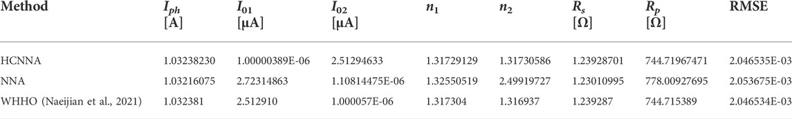
TABLE 3. Comparison of results between HCNNA and other state-of-the-art metaheuristics for the Photowatt-PWP201 PV module with DDM.

Figures 9A,B show the I-V and P-V characteristic curves reconstructed using the parameters estimated by HCNNA for the SDM and DDM with the Photowatt-PWP201 PV module. A good correspondence between experimental and estimated data is clearly observed over the whole voltage range, which shows that the estimated parameters are accurate. HCNNA performed well with both models when estimating the unknown parameters for the Photowatt-PWP201 PV module.

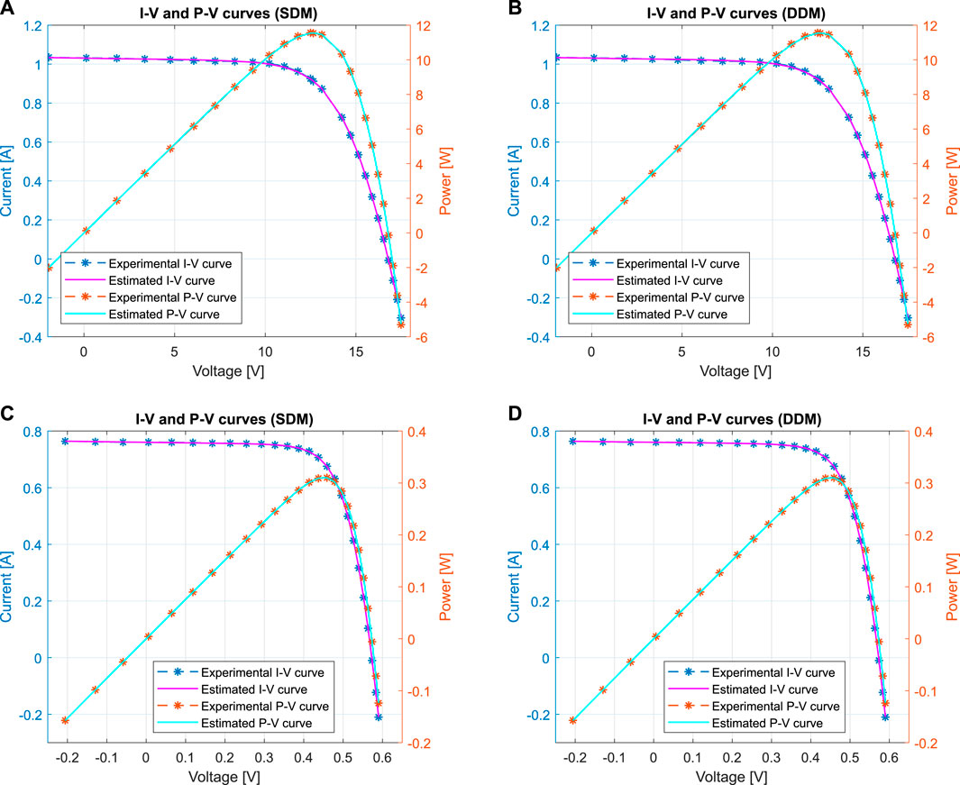
FIGURE 9. Comparisons between experimental and estimated data obtained by HCNNA: (A) Photowatt-PWP201 with SDM; (B) Photowatt-PWP201 with DDM; (C) RTC France with SDM; (D) RTC France with DDM.

For the RTC France PV cell standard dataset, measured under 1000 W/m² irradiance and 33°C temperature (Easwarakhanthan et al., 1986), the PV parameter estimation results with SDM are presented and compared with the ones presented in literature, as shown in Table 4. The results comparison shows that in this case the HCNNA was 91.43% better than the NNA, with RMSE values of 7.730063E-04 and 1.479782E-03, respectively. The MJSO and EMPA obtained similar accuracy to HCNNA, while the remaining methods obtained an RMSE value of approximately 9.860E-04.

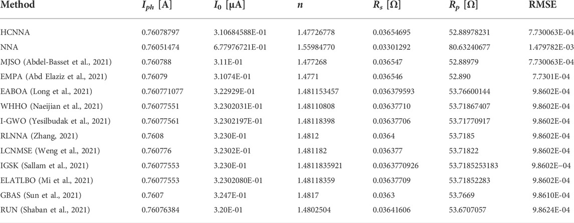
TABLE 4. Comparison of results between HCNNA and other state-of-the-art metaheuristics for the RTC France PV cell with SDM.

Table 5 presents the results with DDM for the RTC France PV cell. As for SDM, the best RMSE value was achieved by HCNNA (7.185582E-04). Comparing this RMSE value with that obtained by the NNA (8.420559E-04) indicates that, for the DDM, the proposed HCNNA was 17.19% better than its ancestor. Both the HCNNA and NNA methods obtained better RMSE value with DDM than with SDM. The MJSO was the second most accurate method (7.419371E-04) and EMPA the third most accurate (7.4396E-04). The remaining methods showed less accuracy, with an RMSE value on the order of 9.8E-04.

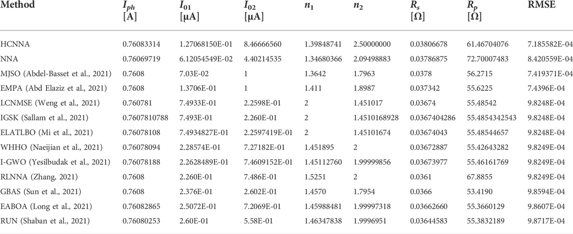
TABLE 5. Comparison of results between HCNNA and other state-of-the-art metaheuristics for the RTC France PV cell with DDM.

Figures 9C,D show the I-V and P-V characteristic curves reconstructed using the parameters estimated by HCNNA for the SDM and DDM with the RTC France PV cell. As with the Photowatt-PWP201 PV module, there was a good correspondence between experimental and estimated data over the whole voltage range, showing that the estimated parameters are accurate. Once again, HCNNA performed well with both models when estimating the unknown parameters for the RTC France PV cell.

Regarding the objective function minimization in the optimal PV parameter estimation, the convergence curves with both models (SDM and DDM) for the HCNNA and NNA are presented in Figure 10. For the Photowatt-PWP201 PV module, the convergence process is presented in Figure 10A. At the beginning of the search process, the HCNNA converged faster than the NNA with both models. Although the HCNNA with the DDM stagnated between iterations 100 and 300, it later surpassed the local optima stagnation, converging on the same value as the SDM. In contrast, the NNA converged prematurely, with both the SDM and DDM. For the RTC France PV cell, the convergence process is presented in Figure 10B and showed a similar behavior. HCNNA was again the fastest at the beginning of the search process, overcoming a possible stagnation zone after a few iterations. Once again, the NNA converged prematurely with both models, which was most evident with the SDM. Overall, the proposed HCNNA clearly achieved more accurate solutions and mitigated premature convergence when compared to the original NNA.

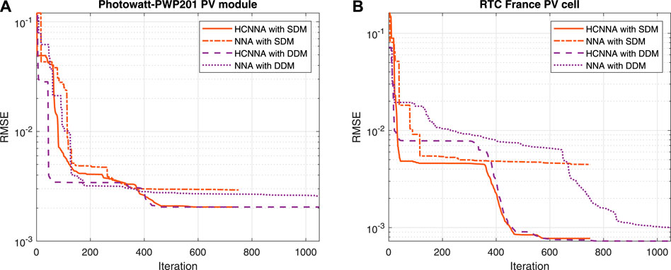
FIGURE 10. Convergence curves of the HCNNA and NNA with SDM and DDM: (A) Photowatt-PWP201 PV module; (B) RTC France PV cell.

5.2 Results with experimental data under partial shading

For the Sharp ND-R250A5 PV module experimental datasets, measured in the irradiance range of 1005 W/m² to 1023 W/m² and temperature range of 48–56°C under partial shading, the electrical characteristics estimation results with SDM are presented in Table 6, specifically the current, voltage and power values for the maximum power point (MPP) of each shading pattern, and the respective individual absolute error (IAE) at the MPP given by Eq. 21.

where I_z represents the experimentally measured current and Î(V_z,τ) the estimated current at each point z of the I-V characteristic curve as a function of the unknown parameters τ.

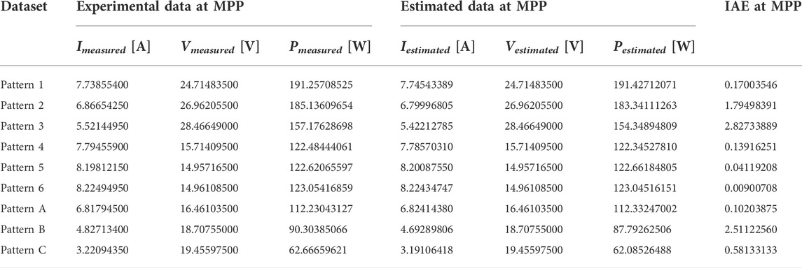
TABLE 6. The measured and estimated current, voltage and power values at MPP, and IAE values for the Sharp ND-R250A5 PV module under partial shading conditions with SDM using the HCNNA.

The results in Table 6 indicate that the IAE at the MPP was 0.09%, 0.97%, 1.80%, 0.11%, 0.03%, 0.01%, 0.09%, 2.78% and 0.93%, for pattern 1 to pattern C, respectively. In fact, the error value was higher than 1% only for pattern 3 (1.80%) and for pattern B (2.78%), demonstrating HCNNA’s good accuracy when estimating the electrical characteristics of the PV module under PSC. The RMSE values considering all points of the I-V characteristic curves are presented later in Section 5.3.

Table 7 presents the electrical characteristics estimation results with the Sharp ND-R250A5 PV module for the DDM. The results were similar to those with the SDM, showing HCNNA’s efficacy and robustness, independently of the PV model. In this case, the IAE at the MPP was 0.07, 0.97, 1.80, 0.06, 0.09, 0.01, 0.11, 2.78 and 0.93%, from pattern 1 to pattern C, respectively. Comparing the error in MPP between both models (SDM and DDM) indicates that the DDM was more accurate for patterns 1 and 4, and performed worse for patterns 5 and A. In the remaining patterns, the accuracy at the MPP was the same in both models.

TABLE 7. The measured and estimated current, voltage and power values at MPP, and IAE values for the Sharp ND-R250A5 PV module under partial shading conditions with DDM using the HCNNA.

The optimal parameters estimated by HCNNA were used to reconstruct the I-V and P-V characteristic curves of patterns 1 to 6 for the SDM and DDM, as shown in Figures 11A–D. The estimated data using both models and the experimentally measured data were coincident for the different shading patterns. The high proximity between the data, regardless of the shading pattern, demonstrates that the proposed HCNNA also obtains accurate results under PSC.

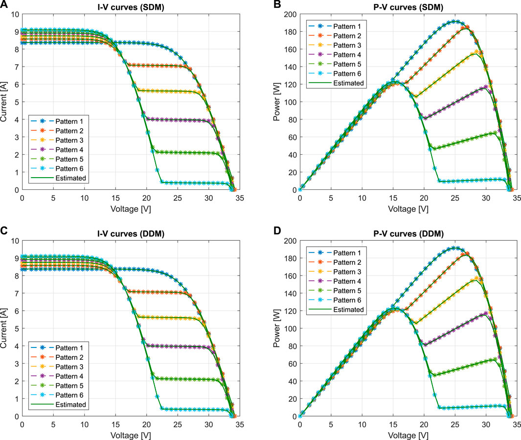
FIGURE 11. Comparisons between experimental and estimated data obtained by HCNNA for the Sharp ND-R250A5 PV module under partial shading (patterns 1–6): (A) I-V curves with SDM; (B) P-V curves with SDM; (C) I-V curves with DDM; (D) P-V curves with DDM.

Figures 12A–D show the I-V and P-V characteristic curves reconstructed using the optimal parameters estimated by HCNNA for patterns A, B and C with the SDM and DDM. A good correspondence between the measured and estimated curves is also inferred in this case and with both models. Although the shading patterns had a greater number of power peaks due to shading of different cell strings, HCNNA maintained a good accuracy.

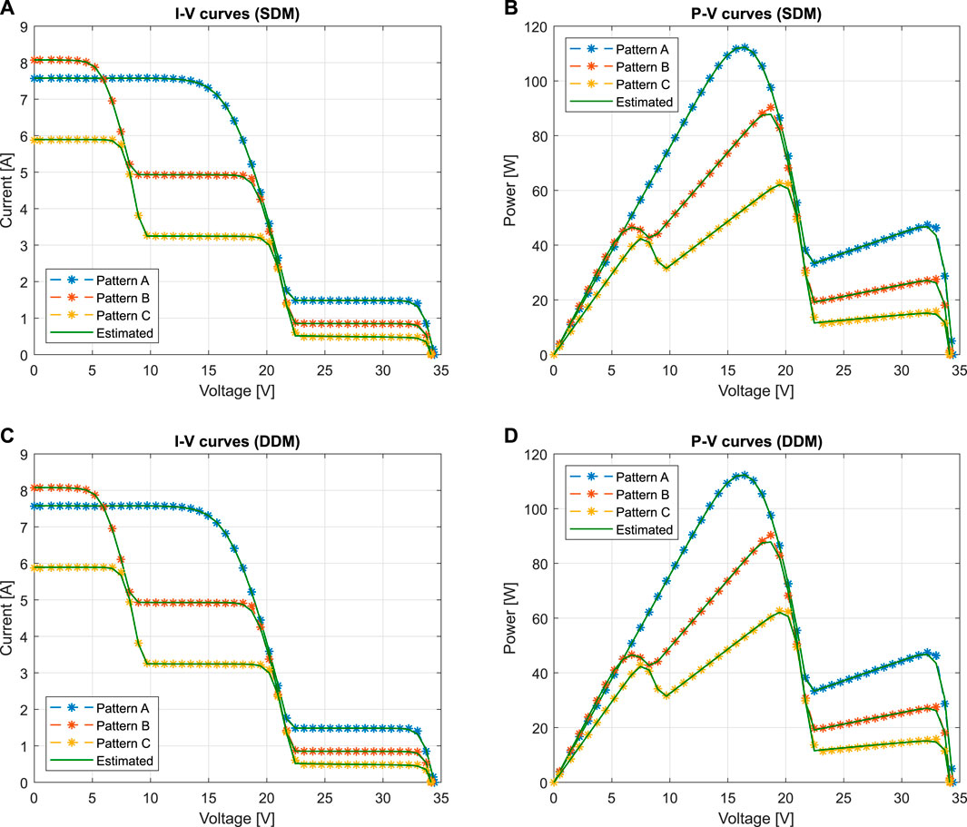
FIGURE 12. Comparisons between experimental and estimated data obtained by HCNNA for the Sharp ND-R250A5 PV module under partial shading (patterns A–C): (A) I-V curves with SDM; (B) P-V curves with SDM; (C) I-V curves with DDM; (D) P-V curves with DDM.

To evaluate the impact of partial shading in terms of efficiency, the PV module efficiency (η) was determined based on the estimated power for each pattern considered through Eq. 22.

where P_MPP is the maximum power value, A the PV module area (m²) and G the incident irradiance (W/m²).

Thus, regardless of the model used (SDM and DDM) the PV module efficiency, η, determined for patterns 1, 2, 3, 4, 5 and 6, was respectively 13.54, 12.41, 10.44, 8.22, 8.16 and 8.31%. While for patterns A, B and C, the efficiency was 8.68, 6.26 and 4.38%, respectively. These results clearly indicate that there is a great loss of efficiency (around 68%) with partial shading.

5.3 Statistical results

In this section, the accuracy, reliability and computational cost of the HCNNA were compared to the original NNA using the standard datasets in the literature (Photowatt-PWP201 PV module and RTC France PV cell) and both models (SDM and DDM). Subsequently, the accuracy and reliability of the HCNNA were evaluated under partial shading using the Sharp ND-R250A5 PV module, also with both models, in a total of nine shading patterns. Specifically, the RMSE statistical results obtained in 30 runs were compared and their distribution analyzed.

Table 8 presents the RMSE statistical results and computational cost for the Photowatt-PWP201 PV module. Considering the minimum RMSE, the HCNNA was 0.43% better than the NNA with the SDM. However, due to the metaheuristic nature of the methods in question, one should consider the mean RMSE, which indicates a 52.77% improvement. For DDM, the HCNNA was 0.35% more accurate than NNA, according to the minimum RMSE, but on average HCNNA was 37.41% more accurate with this model. Analyzing the standard deviation (STD), the HCNNA was not only more accurate, but also more consistent, obtaining an STD of 3.568167E-10 and 6.249338E-08, for the SDM and DDM, respectively. Regarding computational cost, the NNA was, on average, 15.54 and 11.06% more efficient, with the SDM and DDM, respectively.

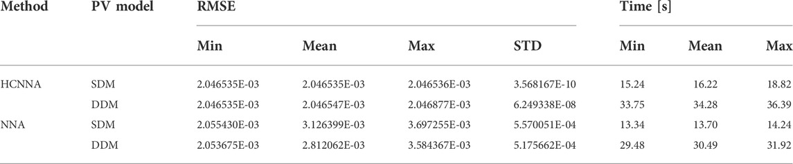
TABLE 8. RMSE statistical results and runtime for the Photowatt-PWP201 PV module with SDM and DDM (30 independent runs).

HCNNA’s robustness with the Photowatt-PWP201 PV module is demonstrated in Figures 13A,B, by the small variation in the RMSE distribution with both models (SDM and DDM), while the NNA presented a large variation. The HCNNA showed very small deviations from the minimum RMSE regardless of the model, therefore it accurately determines solutions by reliably estimating the PV parameters.

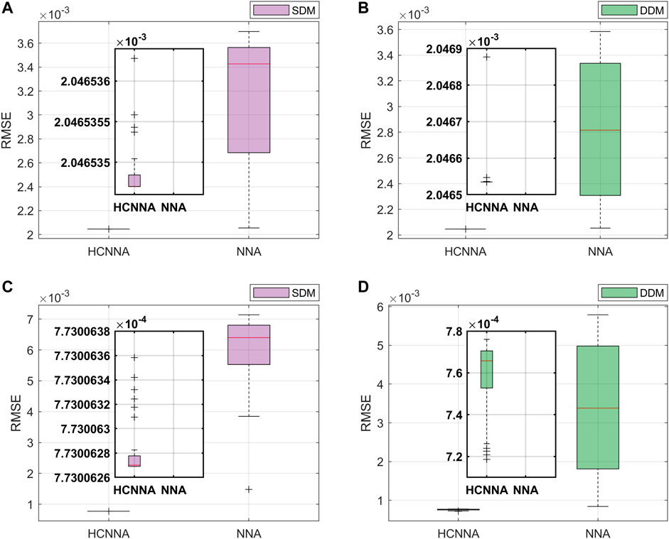
FIGURE 13. RMSE distribution achieved by HCNNA and NNA in 30 runs: (A) Photowatt-PWP201 with SDM; (B) Photowatt-PWP201 with DDM; (C) RTC France with SDM; (D) RTC France with DDM.

For the RTC France PV cell, the RMSE statistical results and computational cost are presented in Table 9. Considering the minimum RMSE, the HCNNA was 91.43% better than the NNA with SDM, while according to the mean RMSE it was 675.39% better. HCNNA was 17.19% more accurate than NNA according to the minimum RMSE with DDM, but on average HCNNA was 343.15% more accurate. Regarding the STD, HCNNA again obtained the best values, and was also the most reliable with the PV cell. The NNA once again presented the best computational cost: 15.09% more efficient than the HCNNA with SDM and 10.83% with DDM.

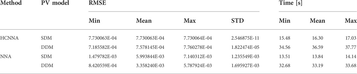
TABLE 9. RMSE statistical results and runtime for the RTC France PV cell with SDM and DDM (30 independent runs).

Figures 13C,D show the RMSE distribution with both models (SDM and DDM) for the RTC France PV cell. Once again, these results clearly show the HCNNA’s robustness. However, with DDM, most of the RMSE values are somewhat far from the minimum value, as indicated by the STD in Table 9. Perhaps the distance between RMSE values and the minimum was related to the fact that the DDM improved accuracy for the PV cell compared to the SDM.

Table 10 shows the HCNNA performance when estimating PV parameters for the Sharp ND-R250A5 PV module under PSC, using SDM and DDM, presenting the RMSE statistical results for each shading pattern. Considering the STD values, the HCNNA was consistent when estimating characteristic curves with multiple power peaks resulting from the use of bypass diodes. To determine the most accurate model, on average, for each of the shading patterns, it is important to compare the mean RMSE values. Thus, the DDM was on average more accurate than the SDM for patterns 3, 4, 5, 6, A and B, respectively 29.46, 0.40, 9.80, 104.72, 5.01 and 19.48% more accurate for those patterns; while the SDM was on average more accurate for patterns 1, 2 and C, respectively 3.54, 8.24 and 17.88%. Overall, this comparison showed that on average the DDM was more accurate under PSC.

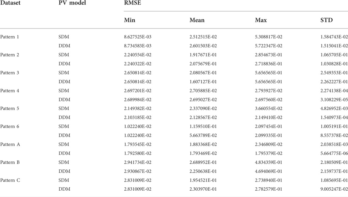
TABLE 10. RMSE statistical results obtained by HCNNA for the Sharp ND-R250A5 PV module under partial shading conditions with SDM and DDM (30 independent runs).

For pattern 1 to 6 (first shading scenario with Sharp ND-R250A5 PV module), the RMSE distribution of HCNNA with both models (SDM and DDM) is shown in Figure 14. SDM and DDM obtained similar RMSE distributions, for patterns 1 and 2. However, for patterns 3, 4 and 6, DDM clearly presented an RMSE distribution closer to the minimum value, compared to SDM. For pattern 5, a similar RMSE distribution was observed with both models, but outliers were observed with the SDM.

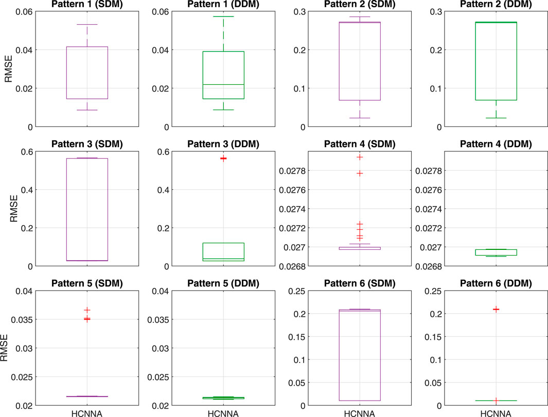
FIGURE 14. RMSE distribution achieved by HCNNA and NNA in 30 runs for the Sharp ND-R250A5 PV module with SDM and DDM under partial shading conditions (patterns 1–6).

Figure 15 presents the RMSE distribution of the HCNNA for the patterns A, B and C with Sharp ND-R250A5 PV module (second shading scenario). Considering patterns A and B, the RMSE distribution was similar with both models (SDM and DDM), although outliers were observed far from the minimum value, with the SDM. As the mean RMSE revealed, HCNNA obtained more accurate solutions with SDM for pattern C.

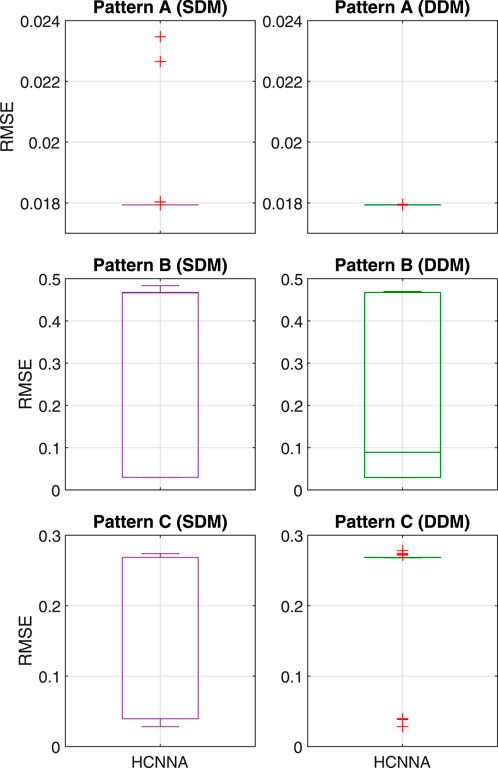
FIGURE 15. RMSE distribution achieved by HCNNA and NNA in 30 runs for the Sharp ND-R250A5 PV module with SDM and DDM under partial shading conditions (patterns A–C).

In summary, the statistical results showed that the proposed HCNNA was significantly more accurate than the NNA when estimating the PV parameters. Furthermore, HCNNA performed well when predicting the PV electrical characteristics under partial shading with SDM and DDM, although that DDM was mostly more accurate under these operating conditions.

6 Conclusion

This paper studied the bypass diode effect on the characteristic curves of photovoltaic (PV) cells or modules and proposed the hill climbing neural network algorithm (HCNNA) to estimate the PV parameters of single- and double-diode models under partial shading conditions. Specifically, the study analyzed the power loss caused by the voltage drop when the bypass diodes switch to the active state due to divergences caused by mismatch or partial shading. The temperature distribution was also analyzed to identify eventual hot spots resulting from these divergences. The proposed HCNNA was validated for estimating the PV parameters, using standard literature data under uniform irradiance and experimentally measured data, with different partial shading patterns. To overcome the implicit nature associated with the PV parameter estimation problem, the Newton-Raphson method was used, and the root mean square error (RMSE) was selected as performance index in the optimization problem.

Results of the bypass diode effect showed power losses up to about 70% with the considered shading patterns, resulting in efficiency losses up to about 68%. Regarding the temperature distribution under partial shading, when the bypass diodes fail, the PV cells can reach very high temperatures. Specifically, in some of the partial shading tests, temperatures of approximately 100°C were reached in a short period of time. The results obtained in the PV parameter estimation demonstrated the HCNNA’s high accuracy and reliability, with and without partial shading. Overall, the performance of the proposed HCNNA was very competitive when compared to other methods in the literature. Considering the standard literature datasets and the minimum RMSE, the HCNNA was on average 27% more accurate when compared to the original NNA. On the other hand, considering the datasets with shading and the mean RMSE, the DDM was on average 28% more accurate than the SDM under partial shading.

In conclusion, the proposed HCNNA demonstrated high performance and reliability, which constitutes a promising alternative to predict the electrical characteristics in PV systems monitoring.

Data availability statement

The raw data supporting the conclusions of this article will be made available by the authors, without undue reservation.

Author contributions

HN and JP contributed to conceptualization and investigation. HN and FM designed the procedure and measured the experimental data. HN and JP developed and validated the proposed methodology. HN and JP were responsible for the original draft preparation. HN, JP, SM and MC reviewed and edited the manuscript. SM and MC performed supervision and resources. All authors read and approved the final manuscript.

Funding

This work is funded by FCT/MCTES through national funds and when applicable co-funded EU funds under the project UIDB/50008/2020.

Acknowledgments

HN gives his special thanks to the Fundação para a Ciência e a Tecnologia (FCT), Portugal, for the Ph.D. Grant (SFRH/BD/140304/2018).

Conflict of interest

The authors declare that the research was conducted in the absence of any commercial or financial relationships that could be construed as a potential conflict of interest.

Publisher’s note

All claims expressed in this article are solely those of the authors and do not necessarily represent those of their affiliated organizations, or those of the publisher, the editors and the reviewers. Any product that may be evaluated in this article, or claim that may be made by its manufacturer, is not guaranteed or endorsed by the publisher.

References

Abd Elaziz, M., Thanikanti, S. B., Ibrahim, I. A., Lu, S., Nastasi, B., Alotaibi, M. A., et al. (2021). Enhanced Marine Predators Algorithm for identifying static and dynamic Photovoltaic models parameters. Energy Convers. Manag. 236, 113971. doi:10.1016/J.ENCONMAN.2021.113971
Abdel-Basset, M., Mohamed, R., Chakrabortty, R. K., Ryan, M. J., and El-Fergany, A. (2021). An improved artificial jellyfish search optimizer for parameter identification of photovoltaic models. Energies 14, 1867. doi:10.3390/EN14071867
Alqaisi, Z., and Mahmoud, Y. (2019). Comprehensive study of partially shaded PV modules with overlapping diodes. IEEE Access 7, 172665–172675. doi:10.1109/ACCESS.2019.2956916
Alweshah, M., Al-Daradkeh, A., Al-Betar, M. A., Almomani, A., and Oqeili, S. (2020). β -Hill climbing algorithm with probabilistic neural network for classification problems. J. Ambient. Intell. Humaniz. Comput. 11, 3405–3416. doi:10.1007/S12652-019-01543-4/TABLES/4
Bai, J., Cao, Y., Hao, Y., Zhang, Z., Liu, S., Cao, F., et al. (2015). Characteristic output of PV systems under partial shading or mismatch conditions. Sol. Energy 112, 41–54. doi:10.1016/J.SOLENER.2014.09.048
Batzelis, E. I., Routsolias, I. A., and Papathanassiou, S. A. (2014). An explicit PV string model based on the Lambert $W$ function and simplified MPP expressions for operation under partial shading. IEEE Trans. Sustain. Energy 5, 301–312. doi:10.1109/TSTE.2013.2282168
Bingöl, O., and Özkaya, B. (2018). Analysis and comparison of different PV array configurations under partial shading conditions. Sol. Energy 160, 336–343. doi:10.1016/J.SOLENER.2017.12.004
Cotfas, D. T., Cotfas, P. A., Oproiu, M. P., and Ostafe, P. A. (2021). Analytical versus metaheuristic methods to extract the photovoltaic cells and panel parameters. Int. J. Photoenergy 2021, 1–17. doi:10.1155/2021/3608138
Easwarakhanthan, T., Bottin, J., Bouhouch, I., and Boutrit, C. (1986). Nonlinear minimization algorithm for determining the solar cell parameters with microcomputers. Int. J. Sol. Energy 4, 1–12. doi:10.1080/01425918608909835
Ishaque, K., Salam, Z., and Taheri, H. (2011). Syafaruddin Modeling and simulation of photovoltaic (PV) system during partial shading based on a two-diode model. Simul. Model. Pract. Theory 19, 1613–1626. doi:10.1016/J.SIMPAT.2011.04.005
Jately, V., Azzopardi, B., Joshi, J., Venkateswaran, V. B., Sharma, A., Arora, S., et al. (2021). Experimental Analysis of hill-climbing MPPT algorithms under low irradiance levels. Renew. Sustain. Energy Rev. 150, 111467. doi:10.1016/J.RSER.2021.111467
Karthick, A., Athikesavan, M. M., Pasupathi, M. K., Kumar, N. M., Chopra, S. S., Ghosh, A., et al. (2020). Investigation of inorganic phase change material for a semi-transparent photovoltaic (STPV) module. Energies 13, 3582. doi:10.3390/EN13143582
Kermadi, M., Chin, V. J., Mekhilef, S., and Salam, Z. (2020). A fast and accurate generalized analytical approach for PV arrays modeling under partial shading conditions. Sol. Energy 208, 753–765. doi:10.1016/J.SOLENER.2020.07.077
Laudani, A., Riganti Fulginei, F., and Salvini, A. (2014). High performing extraction procedure for the one-diode model of a photovoltaic panel from experimental I–V curves by using reduced forms. Sol. Energy 103, 316–326. doi:10.1016/j.solener.2014.02.014
Lee, C. G., Shin, W. G., Lim, J. R., Kang, G. H., Ju, Y. C., Hwang, H. M., et al. (2021). Analysis of electrical and thermal characteristics of PV array under mismatching conditions caused by partial shading and short circuit failure of bypass diodes. Energy 218, 119480. doi:10.1016/J.ENERGY.2020.119480
Li, B., Chen, H., and Tan, T. (2021). PV cell parameter extraction using data prediction–based meta-heuristic algorithm via extreme learning machine. Front. Energy Res. 9, 693252. doi:10.3389/fenrg.2021.693252
Liu, W., Wang, Y., and Song, J. (2021). Research on Schottky diode with high rectification efficiency for relatively weak energy wireless harvesting. Superlattices Microstruct. 150, 106639. doi:10.1016/J.SPMI.2020.106639
Long, W., Wu, T., Xu, M., Tang, M., and Cai, S. (2021). Parameters identification of photovoltaic models by using an enhanced adaptive butterfly optimization algorithm. Energy 229, 120750. doi:10.1016/J.ENERGY.2021.120750
Manokar, A. M., Winston, D. P., Kabeel, A. E., and Sathyamurthy, R. (2018). Sustainable fresh water and power production by integrating PV panel in inclined solar still. J. Clean. Prod. 172, 2711–2719. doi:10.1016/J.JCLEPRO.2017.11.140
Mi, X., Liao, Z., Li, S., and Gu, Q. (2021). Adaptive teaching–learning-based optimization with experience learning to identify photovoltaic cell parameters. Energy Rep. 7, 4114–4125. doi:10.1016/J.EGYR.2021.06.097
Mohammed, H., Kumar, M., and Gupta, R. (2020). Bypass diode effect on temperature distribution in crystalline silicon photovoltaic module under partial shading. Sol. Energy 208, 182–194. doi:10.1016/J.SOLENER.2020.07.087
Moreira, H. S., Lucas de Souza Silva, J., Gomes dos Reis, M. V., de Bastos Mesquita, D., Kikumoto de Paula, B. H., Villalva, M. G., et al. (2021). Experimental comparative study of photovoltaic models for uniform and partially shading conditions. Renew. Energy 164, 58–73. doi:10.1016/J.RENENE.2020.08.086
Naeijian, M., Rahimnejad, A., Ebrahimi, S. M., Pourmousa, N., and Gadsden, S. A. (2021). Parameter estimation of PV solar cells and modules using whippy Harris hawks optimization algorithm. Energy Rep. 7, 4047–4063. doi:10.1016/J.EGYR.2021.06.085
Nunes, H. G. G., Pombo, J. A. N., Mariano, S. J. P. S., and Calado, M. R. A. (2021). Suitable mathematical model for the electrical characterization of different photovoltaic technologies: Experimental validation. Energy Convers. Manag. 231, 113820. doi:10.1016/j.enconman.2020.113820
Nunes, H. G. G., Silva, P. N. C., Pombo, J. A. N., Mariano, S. J. P. S., and Calado, M. R. A. (2020). Multiswarm spiral leader particle swarm optimisation algorithm for PV parameter identification. Energy Convers. Manag. 225, 113388. doi:10.1016/j.enconman.2020.113388
REN21 (2021). Renewables 2021 global status. Paris: REN21 Secretariat. Available at: https://www.ren21.net/reports/global-status-report/ (Accessed March 17, 2022).report
Sadollah, A., Sayyaadi, H., and Yadav, A. (2018). A dynamic metaheuristic optimization model inspired by biological nervous systems: Neural network algorithm. Appl. Soft Comput. 71, 747–782. doi:10.1016/J.ASOC.2018.07.039
Sallam, K. M., Hossain, M. A., Chakrabortty, R. K., and Ryan, M. J. (2021). An improved gaining-sharing knowledge algorithm for parameter extraction of photovoltaic models. Energy Convers. Manag. 237, 114030. doi:10.1016/J.ENCONMAN.2021.114030
Seyedmahmoudian, M., Mekhilef, S., Rahmani, R., Yusof, R., and Renani, E. T. (2013). Analytical modeling of partially shaded photovoltaic systems. Energies 6, 128–144. doi:10.3390/en6010128
Shaban, H., Houssein, E. H., Pérez-Cisneros, M., Oliva, D., Hassan, A. Y., Ismaeel, A. A. K., et al. (2021). Identification of parameters in photovoltaic models through a Runge Kutta optimizer. Mathematics 9, 2313. doi:10.3390/MATH9182313
Sharp (2012). Sharp solar modules. ND-R250A5, 1–2. Available at: http://upkeep.sharp.eu/cps/rde/xchg/eu/hs.xsl/-/html/product_details.htm?product=NDR250A5&cat=46005 (Accessed April 10, 2017).
Sun, L., Wang, J., and Tang, L. (2021). A powerful bio-inspired optimization algorithm based PV cells diode models parameter estimation. Front. Energy Res. 9, 675925. doi:10.3389/fenrg.2021.675925
Wang, Y. J., and Hsu, P. C. (2011). An investigation on partial shading of PV modules with different connection configurations of PV cells. Energy 36, 3069–3078. doi:10.1016/J.ENERGY.2011.02.052
Weng, X., Heidari, A. A., Liang, G., Chen, H., Ma, X., Mafarja, M., et al. (2021). Laplacian Nelder-Mead spherical evolution for parameter estimation of photovoltaic models. Energy Convers. Manag. 243, 114223. doi:10.1016/J.ENCONMAN.2021.114223
Yesilbudak, M., Fernão, V., Colak, I., and Kurokawa, F. (2021). Parameter extraction of photovoltaic cells and modules using grey wolf optimizer with dimension learning-based hunting search strategy. Energies 14, 5735. doi:10.3390/EN14185735
Yousri, D., Fathy, A., Rezk, H., Babu, T. S., and Berber, M. R. (2021). A reliable approach for modeling the photovoltaic system under partial shading conditions using three diode model and hybrid marine predators-slime mould algorithm. Energy Convers. Manag. 243, 114269. doi:10.1016/J.ENCONMAN.2021.114269
Zhang, Y. (2021). Neural network algorithm with reinforcement learning for parameters extraction of photovoltaic models. IEEE Trans. Neural Netw. Learn. Syst. 1, 1–11. doi:10.1109/TNNLS.2021.3109565
Zhang, Y., Su, J., Zhang, C., Lang, Z., Yang, M., Gu, T., et al. (2021). Performance estimation of photovoltaic module under partial shading based on explicit analytical model. Sol. Energy 224, 327–340. doi:10.1016/J.SOLENER.2021.06.019
Keywords: hill climbing neural network algorithm, parameter estimation, single-diode model, double-diode model, bypass diode, partial shading condition
Citation: Nunes HGG, Morais FAL, Pombo JAN, Mariano SJPS and Calado MRA (2022) Bypass diode effect and photovoltaic parameter estimation under partial shading using a hill climbing neural network algorithm. Front. Energy Res. 10:837540. doi: 10.3389/fenrg.2022.837540
Received: 16 December 2021; Accepted: 07 July 2022;
Published: 12 August 2022.
Edited by:
Petru Adrian Cotfas, Transilvania University of Brașov, RomaniaReviewed by:
Minh Quan Duong, University of Science and Technology, The University of Danang, VietnamMuthu Manokar A., B. S. Abdur Rahman Crescent Institute Of Science And Technology, India
Copyright © 2022 Nunes, Morais, Pombo, Mariano and Calado. This is an open-access article distributed under the terms of the Creative Commons Attribution License (CC BY). The use, distribution or reproduction in other forums is permitted, provided the original author(s) and the copyright owner(s) are credited and that the original publication in this journal is cited, in accordance with accepted academic practice. No use, distribution or reproduction is permitted which does not comply with these terms.
*Correspondence: S. J. P. S. Mariano, sm@ubi.pt