An Approach to Solar Radiation Prediction Using ARX and ARMAX Models

1 Introduction

According to Barnaby and Crawley (2011), large-scale climate data measurements historically supported aviation and agricultural activities. However, in architecture or engineering it has been used for only about 40 years. Up until the 1990’s, climate data were mainly collected manually and then the procedures were automated. In Brazil, the availability of data from automatic stations is even more recent, and most automatic stations started acquiring measurements in 2007 (Roriz 2012).

Representativeness is the greatest difficulty related to the data collected, since meteorological data may significantly vary year after year. Thus, it is necessary to identify which data are representative for the local climate (Rossi et al., 2009; Chan 2011). According to Rossi et al. (2009), this climatic representativeness can be obtained by means of statistical methods, such as the climatological normal, the identification of typical days of the project, or by specific methodologies, such as the construction of meteorological archives (Guimarães and Carlo 2015).

Although the methods provided meteorological data representative of the location, the selection of different methods tends to result in climate files with different data. In addition, according to Barnaby and Crawley (2011), meteorological parameters such as ambient temperature and wind speed may differ significantly according to the site of the measurement (Guimarães et al., 2014).

As a physical system, the atmosphere can be described by a system of mathematical equations derived from the application of Newton’s second law and the development of differential calculus (18th century). However, the system of equations that determines atmospheric movements is overly complex. Thus, it cannot be solved in an exact and analytical way and demands a series of approximations (INPE 2016). With the exponential development of technology, computer simulation tools have been used in several areas of knowledge. The main objective of computational simulation is to provide users with results close to real situations by means of tools that seek to provide a solution similar to a realistic model, optimize projects and productive processes. At the same time errors must be minimized and results analyzed long before the start of the project prototyping phase (Carlo and Lamberts 2008; Hensen and Lamberts 2011).

The adjustment of the parameters of a mathematical model used to represent a system is called System Identification (G.J. Ríos-Moreno et al., 2007). According to Ljung (1999), System Identification is grounded in standard statistical techniques, and many of the basic routines have direct interpretations, for example, least squares and maximum likelihood. The control community had an important role in the development and application of these basic techniques to dynamic systems right after the birth and development of modern control theory (Ljung 1999).

A reliable forecast of incident solar radiation, both in buildings and in applications related to agriculture, photovoltaic and solar thermal energy generation, is crucial for projects of interest to these applications (Obukhov et al., 2018). The prediction of meteorological data via computational mathematical models aims to generate a set of numerical values with the same statistical characteristics of a historical series of collected data. A weather forecast is prepared for a certain period, location, or region. Forecasts are associated with a certain degree of uncertainty. These predictions are applied in several areas, including renewable energy generation systems and precision agriculture (Fruteira et al., 2011).

Therefore, according to Fruteira et al. (2011) and Ruslan et al. (2017), the simulated data must undergo a validation process for analysis of their reliability and representation of the actual climatic conditions of the location of interest. This can assure that the statistical properties contained in the historical series of each meteorological variable have been preserved.

In general, several models have been used in the literature to estimate and predict solar radiation. Thus, choosing the best model for each type of application becomes a growing challenge (Belmahdi et al., 2021; Suganthi and Samuel, 2012).

With the advancements in computing technology for data acquisition and processing, the parameters of the structural models can be updated from the responses measured under system excitation. This procedure is obtained using identification techniques as an inverse problem. The inverse problem can be defined as the determination of the internal structure of a physical system from either the measured behavior of the system or the estimation of an unknown input that gives rise to a measured output signal (Khanmirza et al., 2011).

Recent studies have used linear and non-linear algorithms intending to solve the problem of predicting solar radiation: Huang et al. (2021) used different machine learning algorithms and Implications for Extreme Climate Events; Belmahdi et al. (2021) used neural networks to predict daily global solar radiation for twenty-five Moroccan cities; Yang et al. (2021) used Kalman filter photovoltaic (PV) power prediction model based on forecasting experience.

In addition, several solar radiation prediction models have been developed over the years and are categorized into three main models: empirical or analytical models, machine learning models, which use computational intelligence techniques, and satellite remote sensing models (Yang et al., 2020). Thus, the present article sought to perform a study on the prediction of solar radiation using linear modeling (ARX, ARMAX).

2 Methodology

2.1 Meteorological Data and Climate Files

The automatic weather station collects meteorological information every minute (temperature, humidity, atmospheric pressure, precipitation, wind direction and speed, solar radiation), representative of the area in which it is located (Mellit and Pavan 2010; Zanetti et al., 2006). The set of received data is validated by quality control and stored in a database (INMET 2011). Literature analysis reveals that prediction methods are based on historical series of energy generation data. These prediction methods demand a large amount of historical data and computational effort (Yang et al., 2021).

Climate files are a set of meteorological data, usually composed of a typical representative year, expressed through several parameters, including temperature, relative air humidity, solar radiation, wind speed and direction (Guimarães and Carlo 2015). The most common climate files identified in Brazil can be found in the Test Reference Year (TRY) and the Test Meteorological Year (TMY) formats, whose statistical treatments select years and months, respectively, without hourly temperature extremes (Carlo and Lamberts 2008).

2.2 Modeling and System Identification

Control strategies based on predictive models are a class of computational algorithms based on the dynamic behavior of a process explained by a mathematical model (Froisy 2006; Ren et al., 2006). The need for a mathematical model able to adequately describe a process is always a challenge, since the performance of control systems is significantly dependent on the modeling accuracy (Vasquez et al., 2008; Obukhov et al., 2018).

The development of an efficient mathematical model is not an ordinary issue, mainly because the criteria that make it applicable depend not only on its purpose and application (Ruslan et al., 2017). Design of control systems based on predictive models should allow for simulating the dynamic behavior of the process or system under the conditions as close to reality as possible, with the simplest possible model to optimize computational resources (Shakouri and Radmanesh 2009).

The representation theorem can be used to obtain several forms of expressing the mathematical models of a system. The linear mathematical representations most frequently used in system identification (Aguirre 2007) are presented below.

It is usual to describe a linear time-invariant system with a controlled input, U, and an uncontrolled input, i.e., noise, W. These inputs present the direct network gain, G(z) and H(z), respectively. In many cases the noise, also called disturbance, can be described by a steady-state stochastic process with rational spectral density. Thus, the Z-transform of the system output is given by the application of the overlapping theorem of linear systems and defined as the linear combination of the two inputs, Eq. 1:

in which G(z) is the transfer function of the deterministic part of the system, and H (z) is the transfer function of the stochastic part of the system. Both are rational and stable functions.

Assuming that the transfer functions of the deterministic and stochastic parts generally have some poles in common, representation of the system output can be written as follows:

where A(z), B(z), C(z), D(z), F(z) are polynomials as a function of z, whose roots of the denominators and numerators are the poles and zeros of the deterministic and stochastic parts of the system, respectively, and d is the system transport delay. Application of the inverse of the Z-transform and use of the back-shift operator provides:

where $q^{-1}$ is the delay operator defined in a such a way that $y\left(k\right)q^{-1}=y\left(k-1\right)$, $w\left(k\right)$ is the white noise and $A\left(q^{-1}\right)$, $B\left(q^{-1}\right)$, $C\left(q^{-1}\right)$, $D\left(q^{-1}\right)$, $F\left(q^{-1}\right)$ are polynomials defined as follows:

The different identification models used in literature are obtained according to the particular values of the polynomials $A\left(q^{-1}\right)$, $B\left(q^{-1}\right)$, $C\left(q^{-1}\right)$, $D\left(q^{-1}\right)$, $F\left(q^{-1}\right)$.

Identification of systems and processes has the following steps: data acquisition, data processing, selection of the model structure, parameter estimation and model validation. These steps will be discussed in more detail in the methodology section.

2.3 Autoregressive Model With Exogenous Inputs and Autoregressive Model With Moving Average and Exogenous Inputs Models

Several models can represent a system in diverse ways, depending on the perspective considered. Some of the models used to simulate linear systems are autoregressive, including the autoregressive model with exogenous inputs (ARX) and the autoregressive model with moving average and exogenous inputs (ARMAX), state variable and transfer functions models (Aguirre 2007; Jorgensen et al., 2011).

The present work explored the autoregressive models with exogenous inputs (ARX) and autoregressive model with moving average and exogenous inputs (ARMAX). The simplest model that can be adjusted to the data of a sample is an autoregressive model with the inclusion of exogenous variables (ARX–autoregressive with exogeneous inputs) (Piltan et al., 2017).

A time series y(t) generally follows an ARX model when it can be explained by the expression of Eq. 9 (Shumway and Stoffer 2006; Aguirre 2007; Moura and Montini 2012):

where $e\left(t\right)$ refers to white noise.

The application of a unit delay operator $z^{-1}y\left(t\right)=y\left(t-1\right)$, in Eqs 4,5 provides:

Thus, the input-output relationship of the model is given by:

The ARX model can be improved with the use of a moving average applied to the disturbance. Thus, we obtain:

Application of the unit delay in Eqs 4–6, similar to the previous case, yields:

where, $n_a$, $n_b$ and $n_c$ refer to the orders of the models.

Thus, the input-output ratio of the ARMAX (autoregressive–moving-average model with exogenous inputs model) is given by:

The present work used an experimental approach to determine systems for achieving a mathematical model that reproduces the dynamic characteristics of the process under study. It was based on observed variables such as: output signal or controlled variable y(t), the input signal x(t), and the disturbances e(t) (Ljung 1999). Figure 1 shows a general outline of the process used for system identification (Vasquez et al., 2008).

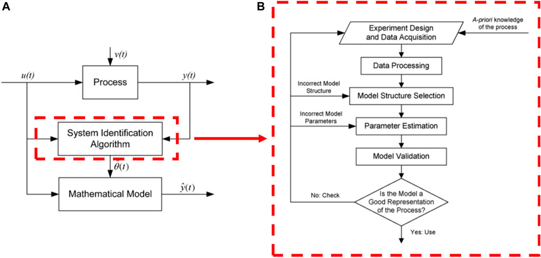
FIGURE 1. (A) System identification process. (B) Steps of the system identification procedure. (Source: Vasquez et al., 2008).

In Figure 1A:

$u\left(t\right)$: System input;

$y\left(t\right)$: System output;

$v\left(t\right)$: Error signal;

$\widehat{\theta }\left(t\right)$: Coefficients generated by the prediction model; and

$\widehat{y}\left(t\right)$: Output generated by the prediction model.

(1) The process for system identification followed the steps below:

(2) Acquisition and modeling of meteorological data: the system must receive external excitation via the application of different input signals and record the evolution of its input and output signals during a predetermined fixed time interval.

(3) Pre-processing of the acquired meteorological data: the acquired data are usually accompanied by unwanted noises and other types of imperfections. Therefore, they must be treated before the start of the identification process.

(4) Definition of the model to be used: it is desirable to obtain a parametric model conditioned to the nature of the data used during the modeling process. Thus, the first step was to determine a structure suitable for the model. For such, it is necessary to acquire previous knowledge of the dynamic behavior of the process under study.

(5) The model parameters were then estimated (specify the names of the parameter here): to allow for determination of the parameter values of the structure that best adapted to the model response for the input and output experimental data.

(6) Then the model was validated, which is the final step. This step sought to determine if the obtained model satisfied the application with the accuracy required for the process. Otherwise, if the obtained model is considered invalid, the following aspects should be analyzed as probable causes:

(i) The input and output data acquired do not provide sufficient information about the dynamics of the system; and/or

(ii) The structure selected was unable to adequately describe the model; and/or

(iii) The criteria for determining the parameters were not properly adjusted.

Thus, depending on the reason an invalid template was obtained, the identification process should be repeated. The system identification process is an iterative process whose steps are illustrated in the flowchart shown in Figure 1B.

2.4 Modeling of the Solar Radiation Database Based on Systems Identification

Initially, the average input and output data were removed in order to normalize the database used. The data were then separated, so that one part was used for simulation and the other for model validation. The percentages used for both simulation and validation were defined according to the size of the database available for the work.

The parameters of the ARX and ARMAX models were simulated using different values of polynomial orders and delays. These values determine the degree of the ordinary differential equation computationally solved for determination of the coefficients of each model. This means that for each value of $n_a$, $n_b$ and $n_c$, a simulation and validation model was created. In the present work the order of the model $\left(n_a,n_b\text{and}{n}_c\right)$ ranged from 1 to 7, while the delay order $\left(n_k\right)$ ranged from 1 to 3. These values are justified by the need for optimizing the use of computational resources, since it is necessary to expand them as the order of the models increases.

The model can be selected by means of the minimal Root Mean Square Error–RMSE. It is a criterion for selecting an appropriate estimator, which means selecting the order of the model to be adopted. The RMSE is the square root of the differences between the estimated value and the actual value of the squared data, weighted by the number of terms and by the estimated value, given by:

Where:$N$ = number of data;$y\left(t\right)$ = original value of each datum; and$y_s\left(t\right)$ = simulated value

This work also used F_IT, an estimator which according to Mustafaraj et al. (2010) and Rachad et al. (2015), is solely the variation of the output generated by the model. In other words, it measures how well the output “fits” the data used in validation of the model. The F_IT is calculated by the equation below:

In statistical modeling, these parameters are used to determine to what extent the model fits the data, or if the removal of some terms could simplify and benefit the model. That is, among other things, it can be used to help determine the variables of interest to be used in the work. It also provides a mechanism for selection of the best estimators (Belmahdi et al., 2021).

In this case, selection depends on the RMSE and F_IT in the ARX and ARMAX models and the degree of each model.

Initially, a treated meteorological database provided by the Laboratory of Technologies in Environmental Comfort and Energy Efficiency of the Department of the Architecture and Urban Planning, Federal University of Viçosa, was used for modeling and data processing. It is important to use a treated meteorological database, since the raw data presented several uncertainties according to the scenario of the measurement and the selection and assembling approach. Gross data tends to present discrepancies, such as measurement errors due to actions outside the meteorological station, sensor failures in data acquisition and equipment defects.

Hourly data was used from 2005 to 2015 including: air temperature (T_air), dew point temperature (T_dp), relative humidity (H_r), atmospheric pressure (P_atm), humidity ratio (h_r), air enthalpy (E_air), specific air mass (ρ), global horizontal radiation, infrared horizontal radiation, extraterrestrial normal radiation, extraterrestrial horizontal radiation, direct normal radiation, diffuse horizontal radiation, global horizontal illuminance, direct normal illuminance, diffuse horizontal illumination, wind direction, wind speed and precipitation.

3 Results and Discussion

In the present work the variables of interest were the radiation compositions, given their importance both for agriculture and the generation of photovoltaic and solar thermal energy. Table 1 shows a sample of the database for a typical day in January 2015. It should be noted that there is a range of variables that can be analyzed.

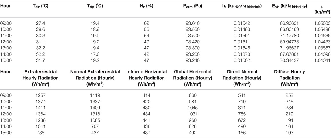
TABLE 1. Sample of hourly weather data for a typical day in January 2015. (Source: Guimarães et al., 2014).

Table 1-Sample of hourly weather data for a typical day in January 2015. Continuation.

Hourly data from 2005 to 2015 were used, containing: Air Temperature (T_air), Dew Point Temperature (T_dp), Relative Air Humidity (H_r), Atmospheric Pressure (P_atm), Enthalpy, Air Density, Global Horizontal Radiation, Horizontal Infrared Radiation, Normal Extraterrestrial Radiation, Horizontal Extraterrestrial Radiation, Direct Normal Radiation, Horizontal Diffuse Radiation, Global Horizontal Illuminance, Direct Normal Illuminance, Horizontal Diffuse Illuminance, Wind Direction, Wind Speed and Precipitation.

Hourly data from all the years were grouped into a single file for simulation. From this, half of the data were used to create the models and the other half for validation. During the simulations, global horizontal radiation was defined as the input and the others as outputs. It must be noted that a new simulation was performed for each variable, Table 2.

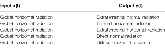
TABLE 2. Inputs and outputs used in the linear modeling.

In each simulation, a sample of 64,992 values was used, of which 32,496 were used to create the model and 32,496 for validation. In validation, the data generated from the models were compared with the existing data by the RMSE analysis and a performance coefficient (F_IT).

In creation of the ARX and ARMAX models, the order of the models $\left(n_a,n_b\text{and}{n}_c\right)$ ranged from 1 to 7, while the delay order $\left(n_K\right)$ ranged from 1 to 3. Therefore, the models were simulated and the RMSE and F_IT values for each model were obtained. Results related to the outputs with the best and worst RMSE were presented for discussion: infrared horizontal radiation and direct normal radiation, according to Tables 3–6.

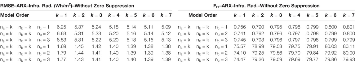
TABLE 3. RMSE and F_IT values for horizontal infrared horizontal radiation model ARX.

TABLE 4. RMSE and F_IT values for horizontal infrared horizontal radiation model ARMAX.

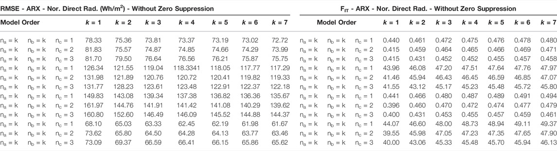
TABLE 5. RMSE and F_IT values for direct normal radiation model ARX.

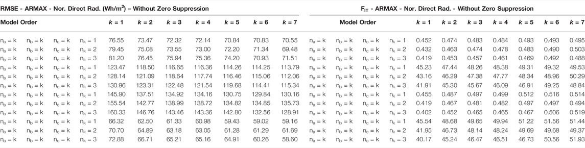
TABLE 6. RMSE and F_IT values for direct normal radiation model ARMAX.

Each model generates 32,496 hourly radiation values, but graphs with 100-h samples were presented in order to facilitate comparison of the original data with that generated by the models. In order to provide a notion of the dimension of the data, Figure 2 shows a graph of 1000 h with all the data.

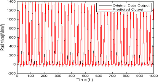
FIGURE 2. Model ARX (na = 4, nb = 4, nc = 3) for prediction of normal extraterrestrial radiation data without zero suppression.

Work involving modeling and identification of systems generally uses analysis of errors to evaluate the quality of the predictors. In the paper published by Mateo et al. (2013), it is suggested to use the absolute mean error as a parameter for the comparison between linear and non-linear predictors. This error measures the average magnitude of the errors in a set of predictions, without considering its direction. Santos et al. (2007) used the comparison between prediction methods based on linear models with an exchange rate approach and used the RMSE as one of the criteria for evaluating the predictors.

Typically, the models of auto regressive prediction try to minimize the prediction errors of a function. The outputs are calculated considering that the system changes slowly over time, by a set of parameters that are estimated via system identification (Huang and Jane 2009).

Comparing the ARX and ARMAX models and graphs applied to the infrared horizontal radiation, it is concluded that in this case it becomes more feasible to use the ARX model, since it requires fewer computational resources than the ARMAX model.

Because zero-suppression infrared horizontal radiation data is all greater than zero, zero suppression was not used in this analysis. As can be seen in Tables 3, 4, the percent difference between the RMSE and F_IT values in the ARX and ARMAX models is not very significant. Both maintain the error below 2% and F_IT around 80%; and errors tend also to stabilize for k = 3. In Figures 3 and 4 it is possible to graphically observe the behavior of mathematically generated data with respect to the data used for validation.

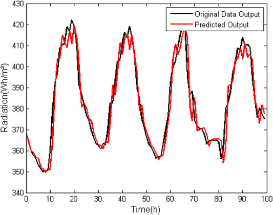
FIGURE 3. ARX model (na = 3, nb = 3, nk = 1) for prediction of horizontal infrared horizontal radiation data without suppression of zero.

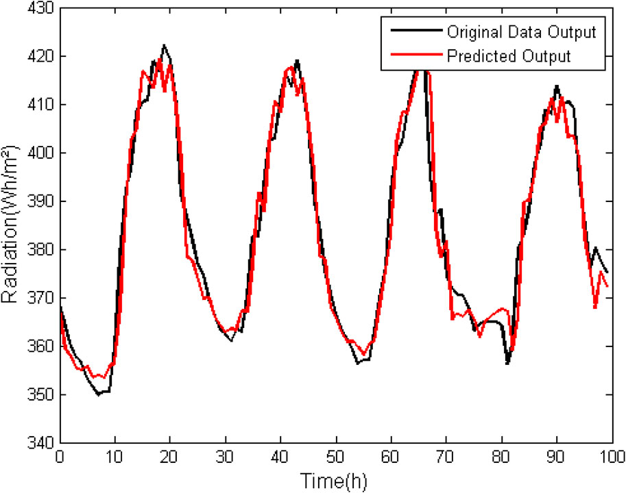
FIGURE 4. ARMAX model (na = 3, nb = 3, nk = 1) for prediction of horizontal infrared radiation data without suppression of zero.

When analyzing Table 5, it can be observed that for the normal direct radiation, in the ARX model without zero suppression the error does not tend to decrease by increasing the order of the model, presenting order values of more than 100% in all degrees of the analyzed model. Furthermore, the F_IT is less than 50% in both cases. Normal direct radiation is of immense importance for simulations in the area of energy efficiency in buildings. Thus, it can be concluded that ARX modeling is not effective in its use for prediction of normal direct radiation data.

In Figures 5, 6 it is possible to graphically observe the behavior of the data generated by the simulation with respect to the data used for validation.

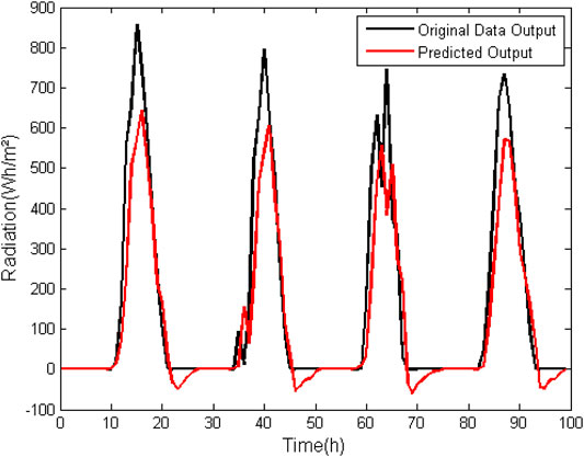
FIGURE 5. ARX model (na = 4, nb = 4, nk = 1) for prediction of normal direct radiation data without suppression of zero.

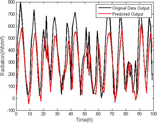
FIGURE 6. ARX model (na = 4, nb = 4, nk = 1) for prediction of normal direct radiation data with suppression of zero.

In the ARMAX model (Table 6) the same effect observed in the ARX model for direct normal radiation composition occurred. Order values of more than 100% were obtained in all grades of the analyzed model. With the suppression of zero the errors become much lower, but they are not yet within an acceptable range. Additionally, the F_IT is less than 50% in both cases. It can therefore be concluded that the ARMAX model generates a poorer approximation than those previously discussed when it comes to their use for prediction of normal direct radiation data.

In Figures 7, 8 it is possible to graphically observe the behavior of mathematically generated data with respect to the data used for validation.

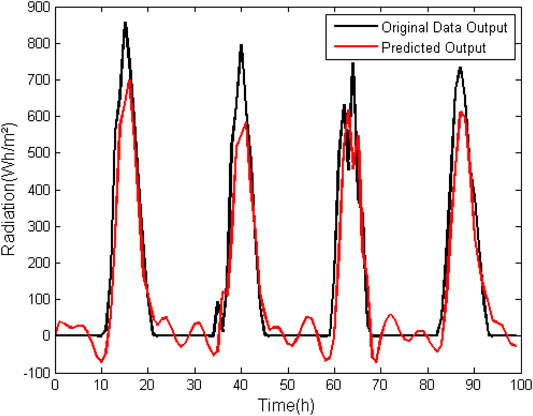
FIGURE 7. ARMAX model (na = 5, nb = 5, nc = 5. nk = 1) for prediction of Normal Direct Radiation data without suppression of zero.

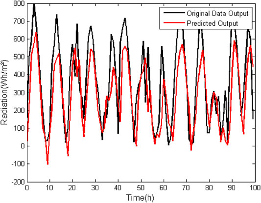
FIGURE 8. ARMAX model (na = 5, nb = 5, nc = 5. nk = 1) for prediction of normal direct radiation data without suppression of zero.

The use of linear modeling (ARX and ARMAX) to predict solar radiation data was efficient for the components: normal, infrared horizontal and horizontal extraterrestrial. For these cases, the smallest errors found between the data used in validation and the data generated by the models, as well as their corresponding F_IT, took into consideration the computational cost-benefit in the choice of k. The best F_IT among the models can be seen in Table 7.

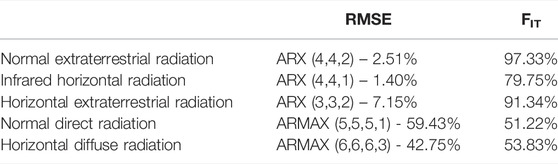
TABLE 7. RMSE and F_IT of the most accurate models for each radiation component generated from horizontal global radiation.

System identification is the procedure of mathematical construction of models, utilizing input and output data previously available for specific analyzes (Haykin 1999; Ljung 1999). Erdoğan and Gülal (2009) defined the system identification as “a matter of finding the numerical values of the model parameters that provide the best agreement between the computed and observed system outputs”.

4 Conclusion

The description of the behavior of meteorological variables, more specifically of solar radiation, is of extreme importance in several areas including aviation, meteorology, power generation, agriculture, hydrology, and others. This description deserves better investigation such as the volume of meteorological data available, since advent of the installation of automatic meteorological stations is still less than expected to increase the level of research that depends on this variable.

Even if there is already a mathematical and physical definition that satisfactorily explains the behavior of solar radiation, it is also necessary to develop and apply predictive methods contribute to the improvement of research that uses solar radiation as the input data variable. The use of RMSE places greater weight on large errors than on small ones, thus emphasizing discrepant data inconsistently with the median of sample data. This explains why the analyzes of horizontal direct radiation and horizontal diffuse radiation have a high RMSE when compared to the others.

Furthermore, a non-sinusoidal arrangement of radiation compositions can be seen graphically in which high RMSE values and low F_IT values were found. This result demonstrates that linear modeling of the ARX or ARMAX type works well for variable databases that vary cyclically, as if it were a composition of sines and cosines.

It was noticed that the ARX or ARMAX linear models worked satisfactorily for databases including variables that vary cyclically, as is the case of most

Data Availability Statement

The raw data supporting the conclusions of this article will be made available by the authors, without undue reservation.

Author Contributions

VS conceived the analysis procedure, provided the analysis tools, the methodology, and the software. DF supervised it giving guidance. JC provided the database. PV has contributed checking the paper for errors and modifying the format of the paper. VS, DF, JC, and PV reviewed the manuscript. All authors read and approved the final manuscript.

Funding

This study was financed in part by the Coordenação de Aperfeiçoamento de Pessoal de Nível Superior - Brasil (CAPES) - Finance Code 001.

Conflict of Interest

The authors declare that the research was conducted in the absence of any commercial or financial relationships that could be construed as a potential conflict of interest.

Publisher’s Note

All claims expressed in this article are solely those of the authors and do not necessarily represent those of their affiliated organizations, or those of the publisher, the editors and the reviewers. Any product that may be evaluated in this article, or claim that may be made by its manufacturer, is not guaranteed or endorsed by the publisher.

Acknowledgments

The authors would like to acknowledge the National Council for Scientific and Technological Development (CNPq), Department of Agricultural Engineering and Department of Architecture and Urbanism of the Federal University of Viçosa (UFV) for their support in development of this work.

Abbreviations

ARX, AutoRegressive model with eXogenous inputs; ARMAX, AutoRegressive Model with Moving Average and eXogenous inputs; RMSE, Root Mean Square Error.

References

Aguirre, L. A. (2007). Introduction to Systems Identification. 3rd ed. Brazil: UFMG. (In Portuguese).
Barnaby, C. S., and Crawley, D. B. (2011). “Weather Data for Building Performance Simulation,” in Building Performance Simulation for Design and Operation. Editors J. Hensen, and R. Lamberts (London, United Kingdom: SponPress), 37–55. chap.3.
Belmahdi, B., Louzazni, M., Akour, M., Cotfas, D. T., Cotfas, P. A., and El Bouardi, A. (2021). Long-Term Global Solar Radiation Prediction in 25 Cities in Morocco Using the FFNN-BP Method. Front. Energ. Res. 9, 733842. doi:10.3389/fenrg.2021.733842
Carlo, J., and Lamberts, R. (20082008). Development of Envelope Efficiency Labels for Commercial Buildings: Effect of Different Variables on Electricity Consumption. Energy and Buildings 40 (11), 2002–2008. doi:10.1016/j.enbuild.2008.05.002
Chan, A. L. S. (2011). Developing a Modified Typical Meteorological Year Weather File for Hong Kong Taking into Account the Urban Heat Island Effect. Building Environ. 46 (12), 2434–2441. doi:10.1016/j.buildenv.2011.04.038
Erdoğan, H., and Gülal, E. (2009). Identification of Dynamic Systems Using Multiple Input–Single Output (MISO) Models. Nonlinear Anal. Real World Appl. 10 (2), 1183–1196. doi:10.1016/j.nonrwa.2007.12.008
Froisy, J. B. (2006). Model Predictive Control Building a Bridge between Theory and Practice. Comput. Chem. Eng. 30 (10–12), 1426–1435. doi:10.1016/j.compchemeng.2006.05.044
Fruteira, R. S., Leite, M. L., and Virgens Filho, J. S. (2011). Performance of the Model PGECLIMA_R in the Simulation of Daily Synthetic Series of Global Solar Radiation for Different Localities of the State of Parana (In Portuguese). Braz. J. Climatology 9 (9), 35–47. Available at: ufpr.br/revistaabclima/article/view/27511/18331. doi:10.5380/abclima.v9i0.27511
Guimarães, I. B. B., Amorim, A. C., and Carlo, J. C. (2014). Statistical and Simulative Comparison of TRY and TMY Climatic Archives Developed for the City of Viçosa-MG. (In Portuguese). Brazil: UFV.
Guimarães, I. B. B., and Carlo, J. C. “Statistical Comparison between Climatic Archives Developed with Different Methods (In Portuguese),” in Proceedings of EURO ELECS - Connecting People and Ideas, Portugal, 2015.
Hensen, J. L. M., and Lamberts, R. (2011). Building Performance Simulation for Design and Operation. Abingdon: Spon Press.
Huang, K. Y., and Jane, C.-J. (2009). A Hybrid Model for Stock Market Forecasting and Portfolio Selection Based on ARX, Grey System and RS Theories. Expert Syst. Appl. 36 (3), 5387–5392. doi:10.1016/j.eswa.2008.06.103
Huang, L., Kang, J., Wan, M., Fang, L., Zhang, C., and Zeng, Z. (2021). Solar Radiation Prediction Using Different Machine Learning Algorithms and Implications for Extreme Climate Events. Front. Earth Sci. 9, 596860. doi:10.3389/feart.2021.596860
INMET (2011). Monitoring of Automatic Stations. Technical Note: 001. (In Portuguese). Available at: www.inmet.gov.br/(Accessed Sept 25, 2016).
INPE (2016). CPTEC - Center for Weather Forecasting and Climatic Studies. Available at: www.cptec.inpe.br (Accessed Jan. 14, 2022).
Jorgensen, J. B., Huusom, J. K., and Rawlings, J. B. (2011). “Finite Horizon MPC for Systems in Innovation Form,” in Proceedings of the 50th IEEE Conference on Decision and Control and European Control Conference (CDC-ECC), Orlando, FL, December 2011. doi:10.1109/CDC.2011.6161509
Khanmirza, E., Khaji, N., and Majd, V. J. (2011). Model Updating of Multistory Shear Buildings for Simultaneous Identification of Mass, Stiffness and Damping Matrices Using Two Different Soft-Computing Methods. Expert Syst. Appl. 38 (5), 5320–5329. doi:10.1016/j.eswa.2010.10.026
Mateo, F., Carrasco, J. J., Sellami, A., Millán-Giraldo, M., Domínguez, M., and Soria-Olivas, E. (2013). Machine Learning Methods to Forecast Temperature in Buildings. Expert Syst. Appl. 40 (4), 1061–1068. doi:10.1016/j.eswa.2012.08.030
Mellit, A., and Pavan, A. M. (2010). A 24-h Forecast of Solar Irradiance Using Artificial Neural Network: Application for Performance Prediction of a Grid-Connected PV Plant at Trieste, Italy. Solar Energy 84 (84), 807–821. doi:10.1016/j.solener.2010.02.006
Moura, F. A., and Montini, A. A. (2012). Application of the Model ARX to Forecast Brazilian Consumption of Industrial Electricity. FACEF Res. Dev. Manag. 15 (2), 192–206. (In Portuguese)Available at: periodicos.unifacef.com.br/.
Mustafaraj, G., Chen, J., and Lowry, G. (2010). Development of Room Temperature and Relative Humidity Linear Parametric Models for an Open Office Using BMS Data. Energy and Buildings 42 (3), 348–356. doi:10.1016/j.enbuild.2009.10.001
Obukhov, S. G., Plotnikov, I. A., and Masolov, V. G. (2018). Mathematical Model of Solar Radiation Based on Climatological Data from NASA SSE. IOP Conf. Ser. Mater. Sci. Eng. 363, 012021. doi:10.1088/1757-899x/363/1/012021
Piltan, F., TayebiHaghighi, S., and Sulaiman, N. B. (2017). Comparative Study between ARX and ARMAX System Identification. Ijisa 9 (No.2), 25–34. doi:10.5815/ijisa.2017.02.04
Rachad, S., Nsiri, B., and Bensassi, B. (2015). System Identification of Inventory System Using ARX and ARMAX Models. Ijca 8 (No.12), 283–294. doi:10.14257/ijca.2015.8.12.26
Ren, Y., Cao, G.-y., and Zhu, X.-j. (2006). Particle Swarm Optimization Based Predictive Control of Proton Exchange Membrane Fuel Cell (PEMFC). J. Zhejiang Univ. - Sci. A. 7 (3), 458–462. doi:10.1631/jzus.2006.a0458
Ríos-Moreno, G. J., Trejo-Perea, M., Castañeda-Miranda, R., Hernández-Guzmán, V. M., and Herrera-Ruiz, G. (2007). Modelling Temperature in Intelligent Buildings by Means of Autoregressive Models. Automation in Construction 16, 713–722. doi:10.1016/j.autcon.2006.11.003
Rodriguez Vasquez, J. R., Rivas Perez, R., Sotomayor Moriano, J., and Peran Gonzalez, J. R. (2008). System Identification of Steam Pressure in a Fire-Tube Boiler. Comput. Chem. Eng. 32 (12), 2839–2848. doi:10.1016/j.compchemeng.2008.01.010
Roriz, M. (2012). Climate Files of Brazilian Municipalities. Available at: http://www.labeee.ufsc.br/downloads/arquivos-climaticos (Accessed Aug 24, 2016).
Rossi, F. A., Dumke, E., and Kruger, E. L. Update of the Reference Climatic Archive for Curitiba. Proceedings of X National Meeting and VI Latin American Meeting of Comfort in the Built Environment. Natal, Brazil. 2009. Available at: https://bv.fapesp.br/pt/auxilios.
Ruslan, F. A., HaronSamad, K., Samad, A. M., and Adnan, R. (2017). “Multiple Input Single Output (MISO) ARX and ARMAX Model of Flood Prediction System: Case Study Pahang,” in Proceedings of the IEEE 13th International Colloquium on Signal Processing & its Applications (CSPA 2017), Penang, Malaysia, 10 - 12 March 2017. doi:10.1109/CSPA.2017.8064947
Santos, A. A. P., da Costa, N. C. A., and Coelho, L. D. S. (2007). Computational Intelligence Approaches and Linear Models in Case Studies of Forecasting Exchange Rates. Expert Syst. Appl. 33 (4), 816–823. doi:10.1016/j.eswa.2006.07.008
Shakouri, G. H., and Radmanesh, H. R. (20092009). Identification of a Continuous Time Nonlinear State Space Model for the External Power System Dynamic Equivalent by Neural Network. Electr. Power Energ. Syst. 31 (7-8), 334–344. doi:10.1016/j.ijepes.2009.03.016
Shumway, R. H., and Stoffer, D. S. (2006). Time Series Analysis and its Applications with R Examples. New York: Springer.
Suganthi, L., and Samuel, A. A. (2012). Energy Models for Demand Forecasting-A Review. Renew. Sustain. Energ. Rev. 16 (2), 1223–1240. doi:10.1016/j.rser.2011.08.014
Yang, L., Cao, Q., Yu, Y., and Liu, Y. (2020). Comparison of Daily Diffuse Radiation Models in Regions of China without Solar Radiation Measurement. Energy 191, 116571. doi:10.1016/j.energy.2019.116571
Yang, Y., Yu, T., Zhao, W., and Zhu, X. (2021). Kalman Filter Photovoltaic Power Prediction Model Based on Forecasting Experience. Front. Energ. Res. 9, 682852. doi:10.3389/fenrg.2021.682852
Keywords: climatic data, predictors, solar radiation, energy, radiation levels
Citation: Silva VLGd, Oliveira Filho D, Carlo JC and Vaz PN (2022) An Approach to Solar Radiation Prediction Using ARX and ARMAX Models. Front. Energy Res. 10:822555. doi: 10.3389/fenrg.2022.822555
Received: 25 November 2021; Accepted: 25 January 2022;
Published: 07 April 2022.
Edited by:
Ravishankar Sathyamurthy, KPR Institute of Engineering and Technology, IndiaReviewed by:
Muthu Manokar A., B. S. Abdur Rahman Crescent Institute Of Science And Technology, IndiaDaniel Tudor Cotfas, Transilvania University of Brașov, Romania
Prasad Chandran, Hindustan University, India
Copyright © 2022 Silva, Oliveira Filho, Carlo and Vaz. This is an open-access article distributed under the terms of the Creative Commons Attribution License (CC BY). The use, distribution or reproduction in other forums is permitted, provided the original author(s) and the copyright owner(s) are credited and that the original publication in this journal is cited, in accordance with accepted academic practice. No use, distribution or reproduction is permitted which does not comply with these terms.
*Correspondence: Delly Oliveira Filho, delly@ufv.br