Influence of installation height of a submersible mixer on solid‒liquid two‒phase flow field

1 Introduction

Submersible mixer is an efficient mixing machinery and pushing device, which plays an essential role in the wastewater treatment process. The impeller of submersible mixer rotates at a high speed driven by the motor, and energy is transferred to the surrounding fluid through the impeller to generate a rotating jet. The jet pushes and reels the surrounding fluid together with low‒speed motion, thus effectively ensuring the suspension of the mixture and promoting sufficient contact and reaction between the sewage and activated sludge.

The flow field inside the pool is exceptionally complicated during the operation of submersible mixer, and experimental studies on it are challenging due to the measurement difficulty and other factors (Tian et al., 2022a). Chen et al. analyzed the effect of impeller diameter on the hydraulic characteristics of a submersible mixer based on STAR‒CCM + simulation software. It was found that the mixer had the best pushing effect when the impeller diameter was 3.7 m in the square pool (Chen et al., 2018). Shi et al. analyzed the mixing flow field of submersible mixers under different pool shapes from the perspective of power consumption. They developed a more suitable pool shape for engineering applications (Shi et al., 2009). Zhang et al. found that by adjusting the placement angle of the submersible mixer, the number and scale of vortices could reduce, which improved the flow pattern at the bottom of the pool and prevented the sedimentation of activated sludge (Zhang et al., 2020). Xu et al. studied the effect of the blade gap on the shaft power, outlet flow rate, and mixing effect of a submersible mixer (Xu and Yuan, 2011). Chen et al. realized the optimal design of the blade airfoil by changing the outlet placement angle of a submersible mixer impeller. It was also verified using numerical simulation to obtain the best airfoil design (Chen et al., 2020a).

To simplify the study, the above studies have used clear water as the study medium. However, the practical application scenario of submersible mixer is sewage‒activated sludge solid‒liquid two‒phase flow. The flow process of sludge particles in the pool is very complex, and the movement is affected by various factors. In studying of the flow field characteristics of submersible mixer, the action of fluid and medium should also be considered, namely, the solid‒phase problem. Therefore, the research on the solid‒liquid two‒phase flow of submersible mixer is of great significance to improve the effect of sewage purification, enhance the purification efficiency and reduce energy consumption.

Currently, two main approaches are used for the study of multiphase flows in fluid mechanics: one is the Euler‒Euler model, which treats both the solid particle phase and liquid phase as continuous phases (Li et al., 2021). The Mixture model based on Euler‒Euler model was primarily adopted for the simulation of the solid‒liquid two‒phase of submersible mixer in the early days (Jin and Zhang, 2014; Tian et al., 2014). The other is Euler‒Lagrange model, which treats solid particles as discrete phase and liquids as continuous phase. Compared with the two‒fluid model, Euler‒Lagrange model successfully introduces particle dynamics, which has the advantages of both macro and micro. It can simulate the actual situation of particle movement in the sewage treatment pool more accurately. The coupled CFD‒DEM (Cundall and Strack, 1979) numerical simulation method based on Euler‒Lagrange framework is now widely used in multiphase simulations in many fields. The model can realistically track the motion of each particle and calculate the collision process between particles by hard or soft sphere model, and the particle rotation can also be captured. With the development of CFD‒DEM technology in recent years, the contact model of particles also introduces rolling friction model for strongly rotating systems, JKR Cohesion model for adhesion and agglomeration between particles containing moisture, and Bonding model for simulating problems such as crushing and fracture, which can analyze the interaction between continuous and discrete phases more accurately. Zhao et al. designed an orthogonal test using a coupled CFD‒DEM method and an integrated Qt‒based simulation platform to investigate the effect of various parameters of the impeller of the stirred kettle on the blending effect of the mixing system (Zhao, 2021). Xia et al. based on the CFD‒DEM coupling method, discussed the flow characteristics of particles in the mixed‒flow pump, the collision form between particles and impeller, and the severe wear area (Xia et al., 2021). Song et al. investigated particle concentration and size effects on the operational performance and wear performance of transfer pumps using coupled CFD‒DEM (Song et al., 2021a). Li et al. used the DEM-CFD coupling method to analyze the internal flow field and particle motion law of a two-stage deep-sea lifting pump at different speeds and studied the secondary flow phenomenon (Yuanwen et al., 2022). Tian et al. studied the solid‒liquid two‒phase flow field of a submersible mixer by using the CFD‒DEM coupling method. They found that the distribution of particles was affected by the vortices in the pool. The particle group easily accumulated around the vortices and near the dead zones of the flow field (Tian et al., 2022b).

In summary, this paper compared and analyzed the motion features of two phases at different installation heights based on the unresolved CFD‒DEM coupled numerical simulation method. At the same time, the mixing degree of activated sludge particles inside the pool is comprehensively evaluated and analyzed using the distribution uniformity method and grey relation analysis method. In addition, the aggregation of particles at different installation heights and the occurring causes are discussed, which has good guidance significance for engineering practice.

2 Calculation model

2.1 Physical model

The pool model and the arrangement of the submersible mixer studied in this paper are shown in Figure 1. The model and arrangement refer to the actual model of a wastewater treatment plant. The size of the pool is the length $L$ = 5 m, width $W$ = 3 m, and effective water depth of $H$ = 2 m. The model of the submersible mixer is simplified for the impeller water body, impeller diameter $D$ = 315 mm, hub diameter $d$ = 105 mm, impeller speed $n$ = 1,600 rpm. The submersible mixer is installed parallel to the bottom of the pool, equal distance from the left and right walls, and the height from the bottom of the pool is h. To study the influence of the installation height of the submersible mixer on the solid‒liquid two‒phase flow field, four schemes are designed, as shown in Table 1.

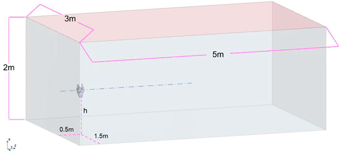
FIGURE 1. Arrangement of pool and submersible mixer.

TABLE 1. Installation height of submersible mixer.

2.2 Mathematical model

2.2.1 Continuous phase mathematical model

In this paper, the continuity equation and momentum equations (Navier‒Stokes equations) are used for the solution of continuous phase. The standard $k-\epsilon$ turbulence model is chosen for the turbulence model.

1) Continuity equation

2) Navier‒Stokes equations

where ${\rho }_f$ is the density of fluid, $u$ is the velocity of fluid, ${\mu }_f$ is the dynamic viscosity of fluid, $p$ is the pressure, and $f$ is the volume force.

3) Turbulence model

In the numerical simulation of submersible mixers, the turbulence model that is currently used is the standard k-ε model (Chen et al., 2016; Gong et al., 2017; Chen et al., 2020a; Zhang et al., 2020). Li compared the difference between the standard k-ε, RNG k-ε, SST, and RSM four turbulence models in the numerical simulation of the stirred kettle with the experimental results. It was found that the results of the pressure and velocity fields predicted using the RSM model and the RNG k-ε model deviated significantly from the actual situation. While the results using the SST model and the standard k-ε model were closer to the actual situation (Li, 2020). In this paper, the standard $k-\epsilon$ turbulence model is used to determine the turbulent viscosity coefficient ${\mu }_t$ using the turbulent energy transport $k$ equation and the energy dissipative transport $\epsilon$ equation. The equations are as follows.

where $G_k$ is the turbulent kinetic energy term generated by the average velocity gradient; ${\sigma }_k$ and ${\sigma }_{\epsilon }$ are the Prandtl numbers corresponding to turbulent kinetic energy and turbulent dissipation rate, respectively; $C_{\mu }$, $C_{1\epsilon }$ and $C_{2\epsilon }$ are empirical constants.

2.2.2 DEM mathematical model

The motion of discrete phase is described by discrete element method (DEM). The motion equations of particles under translation and rotation are as follows (Song et al., 2021b):

where $m_p$ is the particle mass, $v_p$ is the instantaneous particle velocity, $M_d$ is the drag torque, $M_c$ is the contact torque, $F_{drag},F_p,F_g,F_{LR},F_{LS}\mathrm{a}\mathrm{n}\mathrm{d}{F}_c\mathrm{a}\mathrm{r}\mathrm{e}\mathrm{t}\mathrm{h}\mathrm{e}\mathrm{s}\mathrm{u}\mathrm{r}\mathrm{f}\mathrm{a}\mathrm{c}\mathrm{e}\mathrm{a}\mathrm{n}\mathrm{d}\mathrm{v}\mathrm{o}\mathrm{l}\mathrm{u}\mathrm{m}\mathrm{e}\mathrm{f}\mathrm{o}\mathrm{r}\mathrm{c}\mathrm{e}\mathrm{s}\mathrm{a}\mathrm{c}\mathrm{t}\mathrm{i}\mathrm{n}\mathrm{g}\mathrm{o}\mathrm{n}\mathrm{p}\mathrm{a}\mathrm{r}\mathrm{t}\mathrm{i}\mathrm{c}\mathrm{l}\mathrm{e},I_p$ is the rotational inertia of particle, ${\omega }_p$ is the angular velocity of particle.

1. Surface forces

1) Drag force

$F_{drag}$ is drag force of continuous relative discrete phase, defined as follows:

where, $C_d$ is the drag coefficient (Schiller, 1933), $v_f$ is the instantaneous fluid velocity, ${\mathrm{R}\mathrm{e}}_p$ is the particle Reynolds number, and $D_p$ is the particle diameter.

2) Pressure gradient force

$F_p$ is the pressure gradient force, defined as follows:

where $V_p$ is the particle volume and $\nabla p_{static}$ is the gradient of the static pressure in continuous phase.

2. Volume forces

1) Gravitational force

$F_g$ is the gravitational force of particle, defined as follows:

2) Rotational lift force

$F_{LR}$ is the particle rotational lift force, which is the lift due to the change in the flow field’s velocity gradient caused by the particles’ rotation (Oesterlé and Dinh, 1998). The jet of the submersible mixer is rotational, and the particles acquire a large angular velocity after being ejected from the impeller, making the particles still have a high angular velocity in the low Reynolds number regions (Tian et al., 2022b). In these areas, the rotational lift’s influence on the particles’ motion is greater. Therefore, rotational lift should not be neglected in mixing systems with high impeller speeds (Shao et al., 2013). It is defined as follows:

where $\Omega$ is the angular velocity of the particle relative to the fluid and $C_{LR}$ is the rotational lift coefficient.

3) Shear lift force

$F_{LS}$ is the particle shear lift force, which is generated by the velocity gradient perpendicular to the main flow direction (Saffman, 1965). In the flow field of the submersible mixer, a very distinct central jet region exists, and there is a large velocity gradient between this region and the surrounding flow field, so the shear lift force should not be neglected (Zhang et al., 2009; Ren et al., 2021). It is defined as follows:

Where $\mathbf{\omega }$ is the curl of fluid velocity, and $C_{LS}$ is the shear lift coefficient.

4) Contact force

$F_c$ is the contact force. In this paper, the Hertz‒Mindlin no‒slip contact model is chosen, defined as follows (Xia et al., 2021):

where $F_{cn}$ and $F_{ct}$ are normal and tangential contact forces respectively, $Y$ is the equivalent modulus of elasticity, $\mu$ is the Poisson’s ratio, $R_{ab}$ is the equivalent contact radius, $u_n$ is the normal displacement, $u_t$ is the tangential displacement, and $G_{ab}$ is the equivalent shear modulus.

3 Numerical calculation

3.1 Grid

In the simulation calculation, increasing the number of cells can improve the computational accuracy, but the computational time will increase significantly. In addition, the improvement in computational accuracy is not noticeable when the number of cells reaches a specific number. In addition, grid independence verification is required to achieve guaranteed computational accuracy while minimizing the number of cells and improving the quality of the grid. This paper selected the commercial software STAR‒CCM + for grid generation. The pool region was divided by the hexahedral grid, and the impeller region was divided by the polyhedral grid. The polyhedral grid originated from the honeycomb conjecture that the same area can be divided using the least number of perimeters. Compared with the traditional grid, the polyhedral grid has more adjacent cells, and the calculation of gradient and local flow conditions are predicted more accurately. Chen et al. studied the flow field of a submersible mixer using the polyhedral grid for research. They concluded that the polyhedral grid could reduce the computational time and ensure computational accuracy (Chen et al., 2020b; Xu et al., 2021).

Five sets of grids are established, which are 320,438, 621,211, 1,542,649, 2,186,086, and 4,030,726. The grid independence verification was performed by comparing the deviations of the hydraulic thrust and torque of the five sets of models with the actual model (Lin et al., 2021; Zhu et al., 2022). The water thrust of this actual model is 2284 N, and the torque is 109 Nm. The deviation of the numerical simulation results from the actual model parameters under five different sets of grid models is shown in Figure 2. The deviation between the numerically simulated torque and hydraulic thrust and the actual model gradually decreases as the number of cells increases, and the deviation tends to be stable from the third group of models. Taking into account the issues of calculation accuracy and computing capacity, this paper selects the third grid as the simulated object.

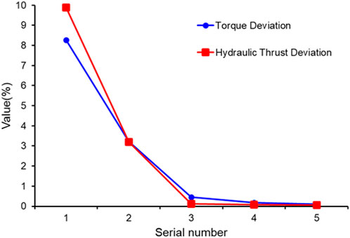
FIGURE 2. Grid independence verification.

3.2 Other settings

The initial conditions of the continuous phase were calculated by the MRF method, and then the sliding grid method was used for the coupling calculation. The impeller area was the rotational domain, and the interface between the pool and the impeller region was set to interface. The free surface of the pool was set by the rigid‒lid assumption, and the remaining walls were set to non-slip walls. The standard $\kappa -\epsilon$ turbulence model was chosen for the turbulence model. The wall treatment was high y + wall treatment, y + > 30, and the continuous convergence residual was set to 10^–4.

The discrete phase was solved using the DEM model. The ejector of particles was located near the water surface, and the particles entered the pool vertically downward from the vicinity of the water surface after the convergence of the continuous phase. The injection time was 4 s. The particles were activated sludge particles and the specific parameters are shown in Table 2. The water surface was set to “phase impermeable” to avoid particles escaping from the water surface, and the rest of the walls were selected to “DEM mode”. The DEM time step was set to 0.000497 s, and the time step of the continuous phase was 0.00497 s. The second‒order implicit unsteady solver was adopted to perform the solution, and the total solution time was 36 s.

TABLE 2. Discrete phase parameters.

4 Result and discussion

4.1 Distribution of the pool flow field

4.1.1 Distribution of velocity

The cross‒section (Y = 0 m plane) along the axis of the impeller and perpendicular to the pool bottom is selected for flow field analysis. The plane’s position is shown in Figure 3. Figure 4 shows the velocity vector of the Y = 0 m plane in the four schemes at 36 s. With the increase in the submersible mixer’s installation position, the jet’s adsorption on the surrounding fluid inhibits the backflow. The vortex above gradually decreases, and the vortex below gradually forms. The jet zone of Scheme 1 and Scheme 2 scour the pool bottom, climb along the pool wall after impacting the wall, and begin to backflow near the pool surface. In scheme 3 and scheme 4, the jet zone is far from the pool bottom, and the development of the jet is less affected by the bottom. It is inferred that the pool has two approximate macroscopic flow patterns due to the different installation heights. Schemes 1 and 2 can be approximated as a single cycle, as shown in Figure 5A, and schemes 3 and 4 can be approximated as a double cycle, as shown in Figure 5B. The single‒cycle flow field has a large vortex, and the double‒cycle flow field has a vortex on each side of the jet.

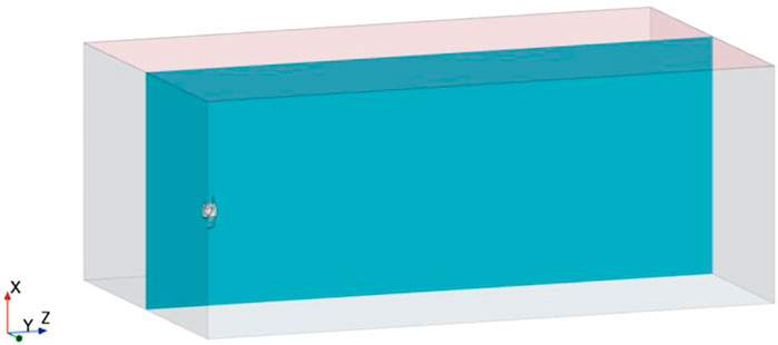
FIGURE 3. Y = 0 plane.

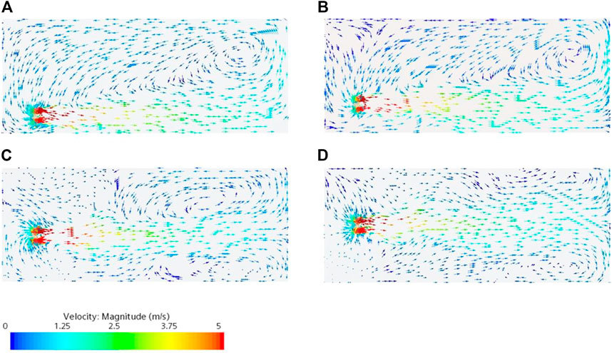
FIGURE 4. Velocity contour maps of Y = 0 plane at 36 s:(A) Scheme 1; (B) Scheme 2; (C) Scheme 3; (D) Scheme 4.

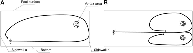
FIGURE 5. Schematic generalization of flow contours: (A) Single cycle; (B) Double cycle.

To evaluate the flow field under the two flow patterns, the average velocity, average turbulent kinetic energy (TKE), velocity distribution uniformity, and turbulent kinetic energy distribution uniformity of the flow field at 36 s were counted. The calculation formula is as follows:

where $v_c$ is the velocity of the fluid in the grid cell, $V_c$ is the volume of the grid cell, $\overline{k}$ is the turbulent kinetic energy of the fluid in the grid cell, and $\overline{v}$, $\overline{k}$, ${\mathrm{\Upsilon }}_v$ and ${\mathrm{\Upsilon }}_k$ are the average velocity, velocity distribution uniformity, average turbulent kinetic energy, and turbulent kinetic energy distribution uniformity of the flow field, respectively.

The statistical results are shown in Figure 6. Scheme 1 and scheme 2 under the single‒cycle flow pattern have higher average velocities, but the uniformity of the velocity distribution, average turbulent kinetic energy, and turbulent kinetic energy distribution are smaller than those of scheme 3 and scheme 4 under the double‒cycle flow pattern. Combined with the vector diagram in Figure 4, it can be analyzed that although the velocity in the flow field of the single‒cycle flow pattern is significant, the velocity direction tends to be consistent, and the turbulence intensity is low. The velocity direction of the flow field in the double cycle flow pattern is chaotic, and the turbulence intensity is high. Its overall velocity and turbulent kinetic energy distribution are uniform, and thus, the mixing performance is better.

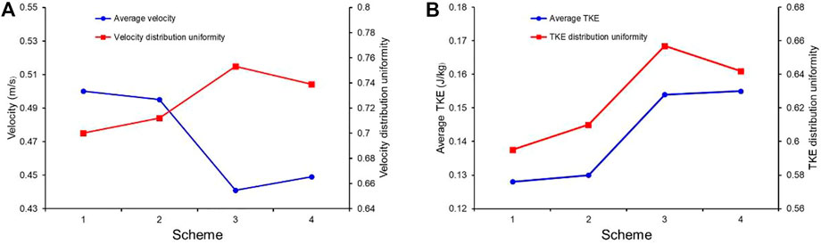
FIGURE 6. (A) Flow field average velocity and velocity distribution uniformity; (B) Flow field average TKE and TKE distribution uniformity.

The flow field distribution at the pool bottom usually significantly influences the solid phase distribution at the bottom (Zhang et al., 2020). Therefore, the flow field on the horizontal cross‒section (x = 0.01 m plane) at 0.01 m from the pool bottom was analyzed, and its location is shown in Figure 7. The velocity contour maps in the x = 0.01 m plane at 36 s for the four schemes are shown in Figure 8. It can be seen that there is a sizeable high‒speed region at the pool bottom for scheme 1 and scheme 2. This region is caused by the effective diffusion radius (ChineseStandard.net, 2007) of the submersible mixer’s rotational jet along the axial development being greater than the installation height and causing the jet to scour the pool bottom. In Schemes 3 and 4, the overall velocity at the pool bottom is lower but more uniformly distributed.

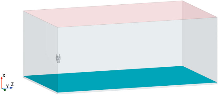
FIGURE 7. X = 0.01 m plane.

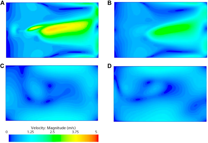
FIGURE 8. Velocity contour maps of X = 0.01 m plane:(A) Scheme 1; (B) Scheme 2; (C) Scheme 3; (D) Scheme 4.

4.1.2 Distribution of dead zones

The purpose of mixing is to transport more kinetic energy to more regions of the flow field. However, due to various factors, there will always be regions with good fluidity and adequate mixing and regions with too low flow velocity, also known as dead zones (Monteith and Stephenson, 1981). The distribution of the dead zone is an important indicator to evaluate the distribution of the flow field. In the field of submersible mixers, the flow field region where the velocity is less than 0.05 m/s is called the dead zone (Tian et al., 2014). Figure 9 shows the distribution of dead zones in the four schemes. The dead zones of the flow field are consistently located, mainly at the pool’s corners, the water surface above the submersible mixer, and the vortex’s core. Figure 10 shows the value of the dead zone volume. The volume size of the dead zone changes with the installation height of the mixer. The dead zone volume of program three is significantly smaller, with a dead zone volume of 0.0765 m³, accounting for 0.25% of the total volume.

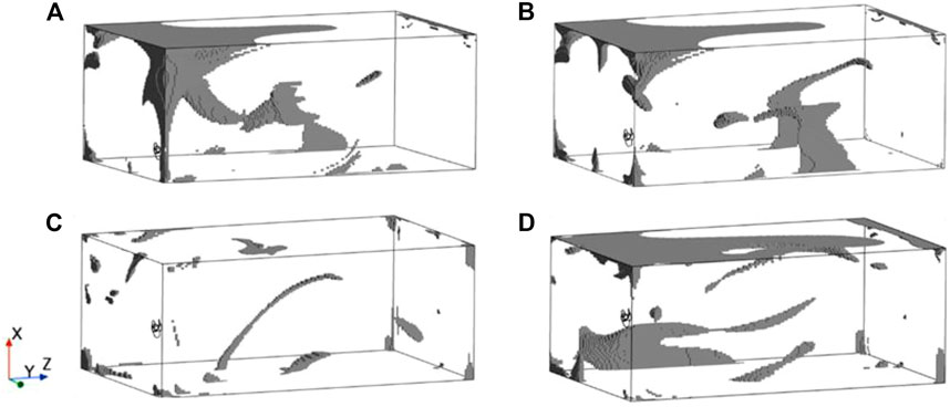
FIGURE 9. Dead zone distribution:(A) Scheme 1; (B) Scheme 2; (C) Scheme 3; (D) Scheme 4.

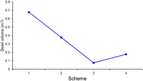
FIGURE 10. Dead zone volume.

4.2 Motion analysis of particles

4.2.1 Particle velocity analysis

Figure 11 shows the variation in the average velocity of particles with time. The average velocity of the particles in schemes 1, 2, and three fluctuates considerably with time, while the average velocity of scheme 4 changes more gently throughout the period. Schemes 1, 2, and three all show one significant decrease in the average velocity of the particles after t = 4 s. The main reason is that 0–4 s is the generation period of the particles. The particles have a vertical downward initial velocity, while the velocity component in the vertical direction of the flow field in this region is low. There is a large slip velocity between the two phases, which leads to a decrease in the average velocity of the particles. Subsequently, the average velocity of particles in schemes 1, 2, and three increased rapidly and gradually reached the peak, but scheme 4 did not show a significant peak. Figure 12 shows the position and velocity distribution of particles at the peak time of each scheme. It can be seen that a large number of particles in schemes 1, 2, and three are inhaled by the impeller and move with the jet, and the particles obtain a large amount of energy. At this time, the particle group moves like a jet in the flow field. In Scheme 4, due to the high installation position, many particles are entrained by the jet and not into the impeller, so there is no prominent velocity peak. After the first peak, the change in the average particle velocity of scheme 2 and scheme 3 gradually stabilized. In contrast, scheme 1 showed a significant peak again, indicating that more particles entered the impeller again. At 36 s, it can be seen that the average velocity of particles in schemes 2, 3, and 4 has reached a relatively stable state, while the average velocity of scheme 1 has a significant increasing trend. Figure 13 shows the velocity and position distribution of the particles in the four schemes at 36 s. Combined with Figure 5, it can be concluded that since scheme 1 is an apparent single‒cycle flow field, a large number of particles move along the wall of the pool, while fewer particles move to the middle of the pool, as shown in the dashed area of Figure 13A Scheme 4 is an apparent double‒cycle flow field. A large number of particles do not enter the impeller, and kinetic energy is obtained mainly through the entrainment of the jet. The particles mainly circulate downstream of the pool, so a sizeable sparse particle area and a low‒speed particle aggregation area appear in the upper area of the impeller, as shown in the dashed area of Figure 13D.

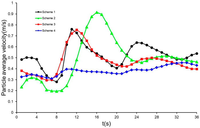
FIGURE 11. 0 s–36 s particle average velocity.

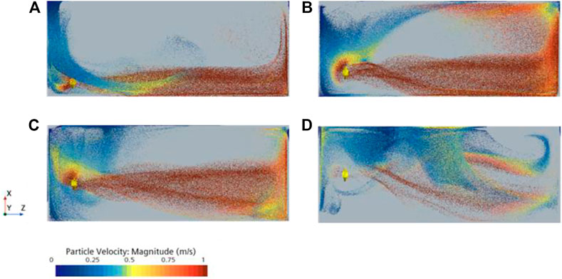
FIGURE 12. Particle distribution and velocity at peak time:(A) Scheme 1:11 s; (B) Scheme 2:16 s; (C) Scheme 3:12 s; (D) Scheme 4:10 s.

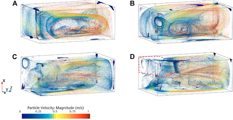
FIGURE 13. Particle position and velocity at 36 s:(A) Scheme 1; (B) Scheme 2; (C) Scheme 3; (D) Scheme 4.

4.2.2 Particle mixing analysis

In this paper, the distribution uniformity method and the grey relation analysis (Zhang et al., 2020) are used to evaluate the mixing degree of particles in pool.

Divide the pool evenly into 3,750 parts. Define each part as a cell, as shown in Figure 14. The number of particles in each cell was counted to calculate the uniformity of particle distribution in the pool. The calculation formula is as follows (Tian et al., 2022b):

where $n_c$ is the number of particles in the cell, $\overline{n}$ is the average number of all cells, and $C$ is the number of cells. The value of ${\mathrm{\Upsilon }}_p$ is larger, indicating that the distribution of particles is more uniform, and the maximum value is 1.

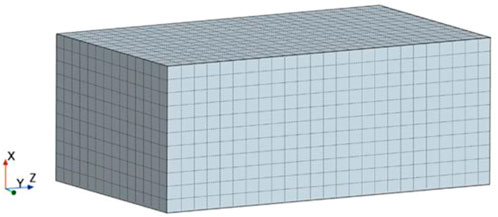
FIGURE 14. Cells of pool.

The variation in particle distribution uniformity with time for the four schemes is shown in Figure 15. The uniformity of the particle distribution of schemes 1, 2, and three is close to stable at t = 33 s, t = 30 s, and t = 27 s, respectively, indicating that the distribution of particles has reached the dynamic equilibrium state at this time, while the distribution of particles of scheme 4 still has not reached the stable state until 36 s. It can be seen that the mixing time for the particles of scheme 3 to reach the stable state is the shortest, and the mixing time of scheme 4 is the longest. At t = 36 s, the particles of scheme 3 had the highest uniformity of distribution with 0.62; scheme 1 had the worst uniformity of distribution with 0.53. The installation height of the submersible mixer has a significant impact on the degree of mixing of particles and mixing time.

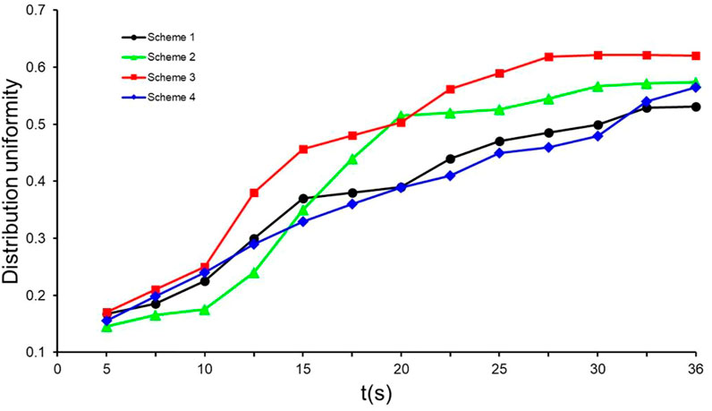
FIGURE 15. Particle distribution uniformity.

The grey relation analysis method is used to evaluate the mixing of particles in the pool (Zhang et al., 2020). The percentage of cells number in different particle number bins constitute a set of sample sequences, with a total of four sets of characteristic sequences. Each group of sequences is recorded as:

where, $l$ is the $l$-th scheme and $k$ is the $k$-th particle number bin, $m$ is the number of schemes and $n$ is the number of particle bins. The details are shown in Table 3.

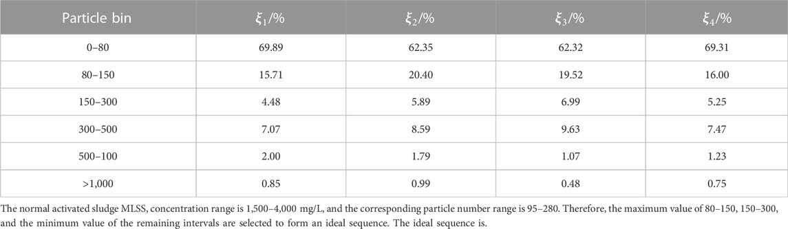
TABLE 3. Percentage of cells number in each particle bin.

The formula for calculating the relevance coefficient ($\mathrm{\Upsilon }$) is as follows:

The formula for calculating the relevancy (${\mathrm{\Upsilon }}_i$) is as follows:

where $\mathrm{\Upsilon }\left({\xi }_0,{\xi }_l\right)$ is the relevancy of ${\xi }_l$ to ${\xi }_0$, its value ranges from 0 to 1, with 0 indicating no correlation and one indicating complete correlation.

Figure 16 shows the relevancy between the characteristic and ideal sequences at different installation heights. From the figure, it can be seen that the highest distribution correlation is 0.936 for scheme 3 and the lowest distribution correlation is 0.607 for scheme 1. The particle distribution inside the pool is closest to the ideal situation when the installation height is 0.8 m as evaluated by the grey relation analysis. The result is consistent with the conclusion reached using the distribution uniformity method, so it can be concluded that the grey relation analysis method can be used to analyze the degree of particle mixing. The grey relation analysis method considers the existence of multiple concentration ranges of solid phase distribution inside the pool. It is suitable for evaluating the mixing of solid phases in the flow field where there are significant core jet zones or high concentration zones.

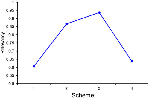
FIGURE 16. Relevancy.

4.2.3 Particle aggregation analysis

Figure 17 shows the distribution of particles inside the pool at 36 s, and the location where particle aggregation occurs can be seen from the figure. The location of particle aggregation changes with the change in installation height, and there are three prominent locations where aggregation occurs, as shown in Figure 18A. These three areas are named the A‒zone, B‒zone, and C‒zone. The number of particles in these three areas is counted, as shown in Figure 18B. It can be found that the least number of particles with aggregation occurs in scheme 1, but the number of particles with aggregation in the A‒zone is more significant than that in the other schemes. Scheme 2 has the highest number of particles with aggregation, and the aggregation of particles mainly occurs in the B‒zone. The number of particles aggregated in Scheme 3 is close to that of Scheme 1, and the particles aggregated mainly in the B‒zone. Scheme 4 has a higher number of aggregated particles, and the main aggregation area of particles is the C‒zone. It is the scheme with the highest number of aggregated particles in the C‒zone among the four groups of schemes.

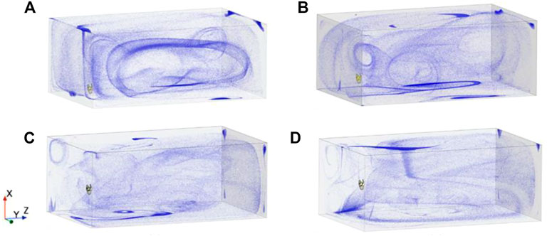
FIGURE 17. Particle distribution at 36 s:(A) Scheme 1; (B) Scheme 2; (C) Scheme 3; (D) Scheme 4.

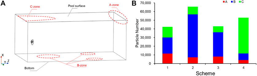
FIGURE 18. (A) Position of particle accumulation zones; (B) Number of particles in the particle accumulation zones.

Figure 19 shows the tracks of the two particles aggregated in the A‒zone during 0–36 s. From Figure 9, it can be seen that the A‒zone of all four schemes is the dead zone of the flow field. Due to the inability to obtain enough kinetic energy, the particles that enter this region directly from the beginning cannot leave and gradually accumulate, as shown in Figure 19A. Some particles enter this region during the backflow process. Due to the large slip velocity between the particles and the flow field in this region, the kinetic energy of the particles decreases and gradually aggregates, as shown in Figure 19B.

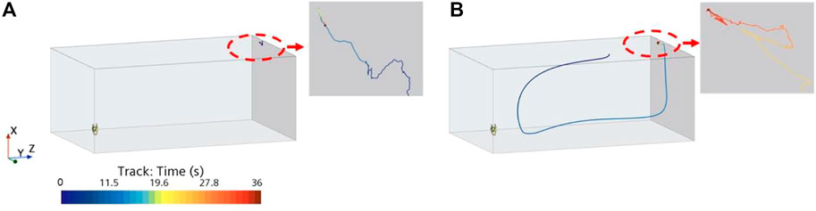
FIGURE 19. Particle track in the A‒zone: (A) Particle track 1; (B) Particle track 2.

Figure 20 shows the particle distribution of the B‒zone in the four schemes. It can be seen that schemes 1 and 2 have similar particle aggregation areas downstream of the pool, named the B₁‒zone. Schemes 3 and 4 have no particle aggregation in this area, but Scheme 3 has a lot of particle aggregation in the middle of the pool bottom, which is named the B₂‒zone. Several particle tracks in Scheme 2, where particle aggregation is more pronounced in the B₁‒zone, are selected, as shown in Figures 21A, B. Combined with Figure 4, it can be seen that the radial disturbance radius of the rotational jet of the submersible mixer gradually increases along the axial direction, and the jet area scours the pool bottom because the installation position is closer to the bottom. Some of the particles carried by the jet will impact the pool bottom together with the jet. After the collision with the pool bottom, the vertical particle velocity decreases to zero, and the particles move forward along the wall of the pool bottom. Combined with the flow field analysis of the bottom area of the pool in Figure 8, the particles moving in the bottom area of the pool eventually gathered in the low‒speed area on both sides of the high‒speed area. The installation position of the submersible mixer in scheme 3 and scheme 4 is higher from the pool bottom, and the particles will not hit the pool bottom with the jet, so no aggregation is formed in the B₁‒zone. The particles in Scheme 3 mainly accumulate in the B₂‒zone, as Figures 21C, D show the tracks of the particles in the B₂‒zone. The particles in Figure 21C are impacted by the jet to the pool bottom and move forward along the wall, and due to the double circulation of the flow field in Scheme 3, the particles are pushed by the return flow below and finally accumulate in the middle of the pool bottom. Figure 21D shows that some particles sink to the pool bottom along the low‒velocity zone near the pool wall and eventually aggregate in the B₂‒zone.

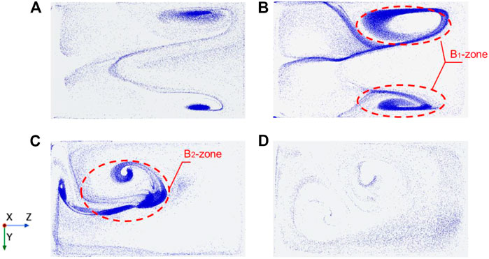
FIGURE 20. Particle distribution in the B‒zone at 36 s (A) Scheme 1; (B) Scheme 2; (C) Scheme 3; (D) Scheme 4.

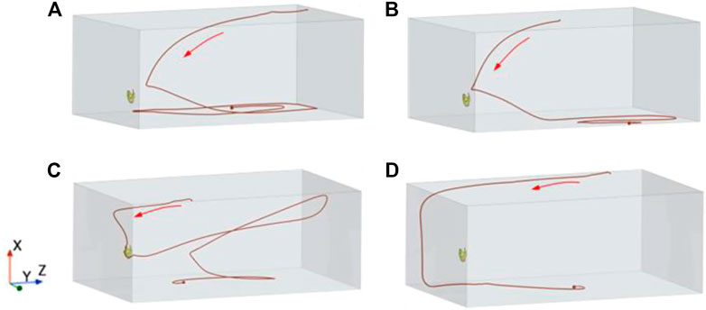
FIGURE 21. Particle track in the B‒zone. (A) Particle track one in the B₁‒zone; (B) Particle track two in the B₁‒zone; (C) Particle track one in the B₂‒zone; (D) Particle track two in the B₂‒zone.

Figure 22 shows the particle distribution in the C‒zone of the four schemes. It can be found that the clustering of scheme 4 is most evident in the region. The 0–36 s track of an aggregated particle in the region of Scheme 4 is selected, as shown in Figures 22A, B is its vertical view. The particle was generated downstream at 3.3 s, reached the aggregation area at 19 s, and then moved at a low speed in this area. Figure 23C shows the flow field in this area. Due to the submersible mixer’s high installation position, a plurality of backflows is formed after the swirling jet impacts the wall surface, in which the two backflows meet upstream to form some low‒speed vortices. Figure 22D is a schematic diagram of vortex formation. Therefore, the particles moving along this path eventually accumulate in the C‒zone.

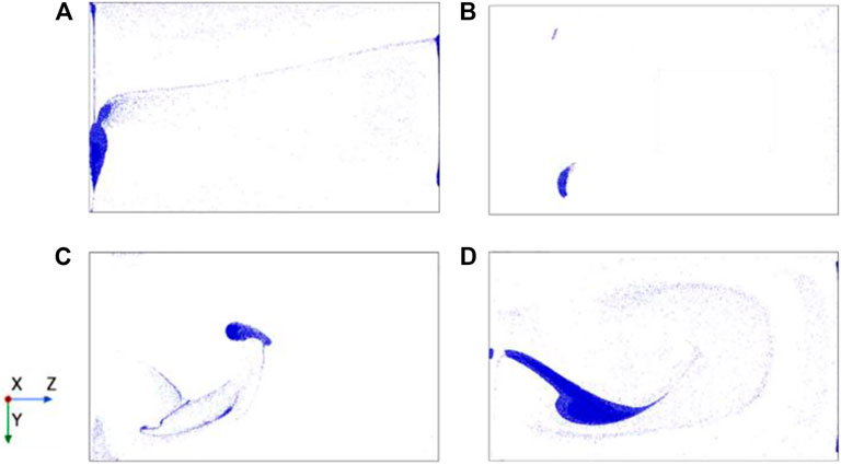
FIGURE 22. Particle distribution in the C‒zone at 36 s (A) Scheme 1; (B) Scheme 2; (C) Scheme 3; (D) Scheme 4.

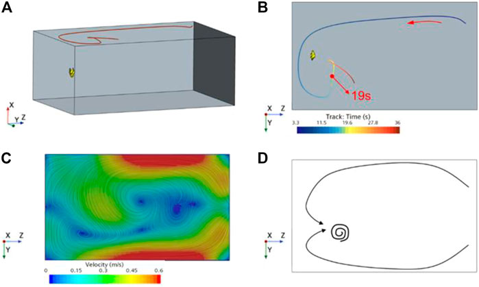
FIGURE 23. (A) Particle track in the C‒zone; (B) Vertical view of particle track; (C) Flow field diagram of C‒zone; (D) Schematic diagram of vortex formation.

Based on the above analysis, it can be seen that the installation height of the submersible mixer greatly influences the movement of the particles. When the installation height is too close to the pool bottom (scheme 1 and scheme 2), the average velocity of particles is high, but the distribution uniformity of particles is poor, and the jet will carry some particles to impact and scour the local area of the pool bottom, resulting in the aggregation of particles. When the installation height is far from the pool bottom (scheme 4), there is no particle aggregation at the pool bottom. Nevertheless, a large amount of particle aggregation occurs upstream of the water surface, and the mixing time and uniformity of the particles are not ideal. Among the four schemes in this paper, scheme 3 is the best because of its ideal mixing time and degree, and the number of particles gathered is less. Therefore, the installation height of the submersible mixer should be greater than the radius of its core jet zone, that is, the effective radial disturbance radius, to avoid the jet zone directly scouring the pool bottom. At the same time, it should not be too far away from the pool bottom to avoid causing the pool surface upstream area of a large number of particles to gather.

5 Conclusion

In this paper, the solid‒liquid two‒phase flow field of submersible mixer installed at different heights is studied by coupled CFD‒DEM. From the perspective of particles, the motion features of particles under different installation heights, the extent of mixing and the reasons for aggregation are analyzed, which has good engineering guidance. The following conclusions can be drawn:

1) With the different installation height of submersible mixer, the flow field inside the pool has single‒cycle and double‒cycle two flow patterns. The double‒cycle flow pattern’s average velocity of the flow field is lower. Still, the average turbulent kinetic energy is higher, and the distribution of velocity and turbulent kinetic energy is better, so the mixing ability of the flow field is stronger.

2) Variations in the installation height of the submersible mixer will affect the time for particles to access the impeller and core jet area and significantly impact the degree of particle mixing, mixing time, and the aggregation intensity of particles. The installation height of the submersible mixer should be greater than its effective jet area’s radius to avoid scouring the pool’s bottom, but it should not be too far from the pool bottom.

3) The method based on the coupling of CFD‒DEM can perform the simulation and study of the solid‒liquid two‒phase flow of submersible mixer effectively. Adjusting the installation position of submersible mixer by using the simulation results can improve the flow pattern inside the pool, improve the mixing uniformity of activated sludge, promote the purification of wastewater, and improve energy utilization efficiency.

Data availability statement

The original contributions presented in the study are included in the article/supplementary material further inquiries can be directed to the corresponding author.

Author contributions

Conceptualization, FT; methodology, FT; software, CY; formal analysis, EZ; investigation, YC and DS; writing—original draft preparation, EZ; writing—review and editing, FT; supervision, WS. All authors have read and agreed to the published version of the manuscript.

Funding

This research was funded by the National Key R&D Program Project (No. 2020YFC1512405), the National Natural Science Foundation of China (No. 51979125), and the Six Talent Peaks Project of Jiangsu Province (JNHB‒192).

Acknowledgments

The authors would like to acknowledge the support received from the National Key R&D Program Project (No.2020YFC1512405), the National Natural Science Foundation of China (No.51979125), Six Talent Peaks Project of Jiangsu province (JNHB‒192).

Conflict of interest

Author YC was employed by the Yatai Pump & Valve Co., Ltd.

The remaining authors declare that the research was conducted in the absence of any commercial or financial relationships that could be construed as a potential conflict of interest.

Publisher’s note

All claims expressed in this article are solely those of the authors and do not necessarily represent those of their affiliated organizations, or those of the publisher, the editors and the reviewers. Any product that may be evaluated in this article, or claim that may be made by its manufacturer, is not guaranteed or endorsed by the publisher.

References

Chen, B., Wang, B. Q., Zhang, H., Wang, Q., and Wang, Z. (2016). Effects of propeller layout position on flow characteristics in oxidation ditch. J. Drain. Irrig. 34 (3), 227–231. doi:10.3969/j.issn.1674-8530.15.0257
Chen, B., Zhuang, Y. F., Chen, K. M., Chen, X. J., and Yang, J. L. (2018). Influence of impeller diameter on hydraulic characteristics of submersible propeller. China Water & Wastewater 34 (5), 57–60.
Chen, Y. F., Cai, X., Zhang, H., Yang, C., Wang, Y., and Xu, Y. F. (2020a). Calculation and analysis of airfoil optimization in artificial flow. J. J. Drainage Irrigation Mach. Eng. 38 (2), 170–175. doi:10.3969/j.issn.1674-8530.19.0185
Chen, Y. F., Yang, Chen., and Zhang, H. (2020b). Influence and optimization of mixer's arrangement of flow field of anoxic pool. J. Drain. Irrig. Mach. Eng. 38, 1045–1050. doi:10.3969/j.issn.1674-8530.19.0210
Cundall, P. A., and Strack, O. D. L. (1979). A discrete numerical model for granular assemblies. Géotechnique 29, 47–65. doi:10.1680/geot.1979.29.1.47
Gong, F. Y., Pan, M. Z., and Tang, L. (2017). Numerical simulation of submersible agitator inside two-dimensional flow field. J. J. Hubei Univ. Technol. 32 (1), 93–96.
Jin, J. H., and Zhang, H. W. (2014). A numerical simulation of submersible mixer in three-dimensional flow with sewage-sludge two-phase. China Rural. Water Hydropower 10, 159–162. doi:10.3969/j.issn.1007-2284.2014.10.0
Li, Q. Y. (2020). Flow field numerical simulation of different turbulent models in miniature reactor based on CFD. J. Contemp. Chem. Ind. 49 (7), 1483–1487. doi:10.3969/j.issn.1671-0460.2020.07.05
Li, W., Wang, L., Shi, W. D., Chang, H., and Wu, P. (2021). Numerical simulation and performance prediction of solid-liquid two-phase flow of alkaline pump based on full factor test. J. Drain. Irrig. Mach. Eng. 39, 865–870. doi:10.3969/j.issn.1674-8530.19.0331
Lin, Y. P., Li, X. J., Li, B. W., Jia, X. Q., and Zhu, Z. C. (2021). Influence of impeller sinusoidal tubercle trailing-edge on pressure pulsation in a centrifugal pump at nominal flow rate. J. Fluids Eng. 143 (9). doi:10.1115/1.4050640
Monteith, H. D., and Stephenson, J. P. (1981). Mixing efficiencies in full-scale anaerobic digesters by tracer methods. J. Water Pollut. Control Fed. 53 (1).
Oesterlé, B., and Dinh, B. (1998). Experiments on the lift of a spinning sphere in a range of intermediate Reynolds numbers. Exp. Fluids 25, 16–22. doi:10.1007/s003480050203
Ren, X. X., Tang, F. P., Xu, Y., Shi, L. J., and Shang, X. J. (2021). Performance analysis of blade angle of submersible agitator. J. South-to-North Water Transfers Water Sci. Technol. 19, 805–813. doi:10.13476/j.cnki.nsbdqk.2021.0084
Saffman, P. G. (1965). The lift on a small sphere in a slow shear flow. J. Fluid Mech. 22, 385–400. doi:10.1017/s0022112065000824
Schiller, V. L. (1933). Uber die Grundlegenden Berechnungen bei der Schwerkraftaufbereitung. Z. Vernes Dtsch. Inge 77, 318–321.
Shao, T., Hu, Y. Y., Wang, W. T., Jin, Y., and Cheng, Y. (2013). Simulation of solid suspension in a stirred tank using CFD-DEM coupled approach. Chin. J. Chem. Eng. 10, 1069–1081. doi:10.1016/s1004-9541(13)60580-7
Shi, W. D., Tian, F., Cao, W. D., Chen, B., and Zhang, D. S. (2009). Numerical simulation of mixer power consumptions in different ponds. J. J. Drainage Irrigation Mach. Eng. 27 (3), 140–144.
Song, L. B., Teng, S., Cao, Q., Kang, C., Ding, K. J., and Li, C. J. (2021a). Wear of large solid particles on the impeller of solid-liquid two-phase flow pump. J. Drain. Irrig. Mach. Eng. 39, 987–993.
Song, L. B., Teng, S., Cao, Q., Kang, C., Ding, K. J., and Li, C. J. (2021b). Solid-liquid two-phase flow characteristics in pipe during large solid particles lifting. J. Drain. Irrig. Mach. Eng. 39, 1111–1117. doi:10.3969/j.issn.1674-8530.20.0278
Tian, F., Shi, W., Jiang, H., and Zhang, Q. (2014). A study on two-phase flow of multiple submersible mixers based on rigid-lid assumption. Adv. Mech. Eng. 2014, 531234. doi:10.1155/2014/531234
Tian, F., Zhang, E. F., Yang, C., Shi, W. D., and Zhang, C. H. (2022a). Review of numerical simulation research on submersible mixer for sewage. Front. Energy Res. 9. doi:10.3389/fenrg.2021.818211
Tian, F., Zhang, E. F., Yang, C., Shi, W. D., and Chen, Y. H. (2022b). Research on the characteristics of the solid-liquid two-phase flow field of a submersible mixer based on CFD-DEM. Energies 15 (16), 6096. doi:10.3390/en15166096
Xia, C., Zhao, R. J., and Shi, W. D. (2021). Numerical investigation of particle induced erosion in a mixed pump by CFD-DEM coupled method. J. Eng. Thermophys. 42, 357–369.
Xu, D. E., Yang, C. X., Cai, J. G., Han, Y., and Ge, X. F. (2021). Numerical simulation of solid-liquid two-phase in tubular turbine. J. Drain. Irrig. Mach. Eng. 39, 910–916. doi:10.3969/j.issn.1674-8530.20.0152
Xu, W. X., and Yuan, S. Q. (2011). Optimization design of submersible mixer based on a simulation study of agitated and engineering application. China Rural. Water Hydropower 06, 32–35.
Yuanwen, L., Zhiming, G., Liu, S., and Xiaozhou, H. (2022). Flow field and particle flow of two-stage deep-sea lifting pump based on DEM-CFD. Front. Energy Res. 10, 10. doi:10.3389/fenrg.2022.884571
Zhang, Y., Jin, B. S., Zhong, W. Q., Ren, B., and Xiao, H. (2009). DEM simulation of particle mixing in flat-bottom spout-fluid bed. Chem. Eng. Res. Des. 88 (5), 757–771. doi:10.1016/j.cherd.2009.11.011
Zhang, Z., Zheng, Y., Jiang, J. Q., and Li, C. Y. (2020). Influence of wastewater mixer setting angle on flow field in sewage treatment pool. J. Drain. Irrig. Mach. Eng. 38, 271–276. doi:10.3969/j.issn.1674-8530.18.0143
Zhao, L. J. (2021). Numerical simulation for stirred mixing based on CFD-DEM and development of integrated simulation platform. Hangzhou, China: Zhejiang University of Technology.
Keywords: submersible mixer, CFD-DEM, two-phase, distribution uniformity method, grey relation analysis
Citation: Tian F, Zhang E, Yang C, Sun D, Shi W and Chen Y (2023) Influence of installation height of a submersible mixer on solid‒liquid two‒phase flow field. Front. Energy Res. 10:1095854. doi: 10.3389/fenrg.2022.1095854
Received: 11 November 2022; Accepted: 28 November 2022;
Published: 23 January 2023.
Edited by:
Kan Kan, College of Energy and Electrical Engineering, ChinaReviewed by:
Wei Jiang, Northwest A&F University, ChinaXiaojun Li, Zhejiang Sci-Tech University, China
Shi Lijian, Yangzhou University, China
Copyright © 2023 Tian, Zhang, Yang, Sun, Shi and Chen. This is an open-access article distributed under the terms of the Creative Commons Attribution License (CC BY). The use, distribution or reproduction in other forums is permitted, provided the original author(s) and the copyright owner(s) are credited and that the original publication in this journal is cited, in accordance with accepted academic practice. No use, distribution or reproduction is permitted which does not comply with these terms.
*Correspondence: Erfeng Zhang, 2222006046@stmail.ujs.edu.cn