MVMO-Based Identification of Key Input Variables and Design of Decision Trees for Transient Stability Assessment in Power Systems With High Penetration Levels of Wind Power
 Da Wang1
  José L. Rueda Torres
- 1Department of Electrical Sustainable Energy, Delft University of Technology, Delft, Netherlands
- 2TenneT TSO B.V., Arnhem, Netherlands
Unlike synchronous generators, wind turbines cannot directly respond to large disturbances, which may cause transient instability, due to their power electronic-based interface and maximum power control strategy. To effectively monitor the influence of wind turbines, this paper proposes an approach that combines decision trees (DTs), and a newly developed variant of the Mean-Variance Mapping Optimization (MVMO) algorithm, to simultaneously tackle the problem of selecting the key variables that properly reflect the transient stability performance of a system dominated by wind power, and designing the DTs for reliable online assessment of transient stability. The notion of key variables refers to the set of variables that are closely related to the modified power system transient stability performance as a consequence of the replacement of conventional power plants by wind generators. The selection of key variables is formulated as a non-linear optimization problem with weight factors as decision variables and is tackled by MVMO. A weight factor is assigned to each key variable candidate, and its value is considered to reflect the degree of influence of the key variable candidate on the splitting property and estimation accuracy of the DTs. The samples of the key variable candidates and the initialized weight factors are used to build the first group of DTs. Then, MVMO iteratively evolves the weight factors according to its special mapping function with minimizing DTs' estimation error. According to the final list of optimized weight factors, system operators can select a reduced set of variables with the largest weight factors as key variables, depending on the resulting accuracy of the DTs. Meanwhile, DTs built by using key variables are considered as the optimal performance trees for transient stability estimation. In this way, the selection of key variables and the development of DTs are made jointly and automatically, without the interference of the users of the DTs. Test results on the modified IEEE 9 bus system and a synthetic model of a real power system show that the proposed method can correctly identify the set of key variables related to wind turbine dynamics, as well as its ability to provide a reliable estimation of the transient stability margin.
Introduction
Transient stability concerns with the ability of synchronous generators to remain in synchronism after being subjected to a large disturbance, such as a three-phase short circuit or a transmission line tripping (Kundur et al., 2004). When such a disturbance occurs, the equilibrium between the mechanical and the electrical torques in each synchronous generator is significantly disturbed, which forces some generators to accelerate and others to decelerate. If the relative motions cannot be attenuated, transient instability (i.e., loss of synchronism) occurs.
As a result, transient instability can lead to generator outages, transmission lines tripping, load shedding, and even blackouts. Significant research efforts have been devoted to efficiently monitor and estimate the degree of transient stability in order to enable system operators to take necessary controls to avoid the occurrence of transient instability (Oluic et al., 2017; Velez et al., 2017). A significant research effort has been devoted to power systems dominated by synchronous generators. Nevertheless, the massive integration of wind power imposes the new challenge on transient stability, because of the different operation and control characteristics from conventional synchronous generators.
The rotator behavior of synchronous generators is directly coupled to the dynamics of electromagnetic power at the terminal bus, via the internal flux linkage (Kundur et al., 2004). It enables the rotor to promptly respond to power fluctuations at the generator's terminal bus in the form of absorbing or releasing kinetic energy, i.e., inertia response. This helps to balance the post-disturbance power flow and improve transient stability. However, the rotor response of the wind turbine is decoupled from power grid dynamics, because of the maximum power pointing track (MPPT) and power electronics interface (Cirrincione et al., 2015; Huang et al., 2015). So, essentially, wind turbines cannot directly provide inertial response like synchronous generators. From this perspective, the replacement of synchronous generators by wind turbines is expected to worsen the transient stability performance of power systems.
On the other hand, the underlying cause of transient instability is the electrical-mechanical power imbalance, due to fluctuations of electromagnetic power at the generator's terminal bus. The electromagnetic power is influenced by all generation/load sources connected to the same transmission network. Therefore, there also exist some possibilities for wind turbines to bring forth positive influences on transient stability. That is to say, regulating the wind turbine output may alleviate the power imbalance of the synchronous generator when a disturbance occurs.
Wind power is in essence highly variable. In Shi et al. (2014), different wind speeds are sampled by the Monte Carlo method and simulated in different operating conditions to obtain the probabilistic profile of transient stability indicators after integrating wind turbines. To get more statistical information about the influence of wind farms on transient stability, different sizes, locations and control parameters of wind farms are simulated in different operating conditions with possible fault scenarios in Meegahapola et al. (2008), Shewarega et al. (2009), and Faried et al. (2010). Unlike the aforesaid sampling-based method, the references (Lin et al., 2013; Liu et al., 2016) formulate analytically the influence of wind turbine on the rotor motion of synchronous generators, which makes possible to use equal area criterion to quantitatively judge transient stability.
However, the influence of wind turbines on transient stability depends on the dynamic properties of each power system: e.g., wind turbine locations, sizes, controllers' parameters, as well as the pre-disturbance system operating conditions. In order to ensure the transient stability of power systems, such an influence should be closely monitored and reliably estimated. This causes two questions: which variables should be monitored? and how to estimate reliably transient stability?
Ideally, monitored variables should be able to cover adequate information for making a reliable estimation of transient stability under a given operating condition. Bus voltage, line current, generator accelerating speed, etc., all could be candidates. However, the use of a large number of variables requires much more computation resources. Therefore, one pragmatic solution is to select a small set of key variables that needs less computation resources, but, nevertheless, enables a reliable estimation for transient instability. The methods to estimate transient stability can be classified into model-based methods (Vu and Turitsyn, 2016) and artificial intelligence-based methods (Hoballah and Erlich, 2012; Cepeda et al., 2014; Wang et al., 2016). The latter requires reduced computation effort to make fast estimations.
This paper proposes a new approach that jointly solves the selection of key variables and the estimation of transient stability by combining a selected method from computational intelligence, i.e., decision trees (DTs), with a powerful optimization tool, MVMO (Mean-Variance Mapping Optimization). Other methods from computational intelligence could also be used, e.g., support vector machine. Nevertheless, the focus of this paper provides insight into how optimization can improve to achieve an optimal performance of a selected computational intelligence method when challenged to provide confident transient stability assessment in systems with very high penetration of power electronic interfaced generation. A detailed comparison with other options with data mining based algorithms or other forms of decision trees, e.g., like algorithms presented in Kamwa et al. (2010) and Rahmatian et al. (2017), is a topic for future research after this paper. Particularly, a group of variables related to transient stability are selected as key variables candidates to build DTs. Each of them is assigned a weight factor. MVMO optimizes these weight factors toward reducing the estimation errors of DTs. Finally, an optimal list of weight factors is obtained. System operators can select a number of variables with the largest weight factors as the key variables to be measured, depending on their communication infrastructure and the estimation accuracy of DTs. At the same time, DTs taking the key variables as the inputs are considered as the optimal performance trees, which are adopted for fast estimation of transient stability.
The rest of the paper is organized as follows. Section Illustration of the Influence of WT on Power System Transient Stability first describes the used WT model and its influence on transient stability. Next, the proposed method is introduced in section The Combined Key Variable Identification and DT Designs, in terms of the mathematic formulation, the algorithm flow, DTs and MVMO. The proposed approach is firstly tested on a modified version of the IEEE 9 bus system in section Test Results on IEEE 9 Bus System. Section Test Results on Great Britain (GB) System provides the results obtained on a reduced size model of a real power system. Section Transient Stability Assessment discusses the possible implementation of the proposed method. Finally, conclusions and future work are given in section Implementation of the Proposed Approach.
Illustration of the Influence of Wt on Power System Transient Stability
Wind Turbine Model
Figure 1 shows the main components of investigated WT type 4 (WT4): wind turbine (WT), gearbox (GB), permanent magnet synchronous generator (PMSM), machine side rectifier (MSR), and grid side inverter (GSI).
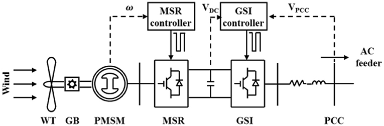
Figure 1. Wind turbine type 4.
The MSR controller regulates the stator currents and thus controls the rotation speed of PMSM to regulate the extracted mechanical power. On the other hand, the GSI controller is responsible to regulate the active power and reactive power injected to the grid. This wind turbine is simulated by an industrial-level PowerFactory model, developed on the basis of IEC 614000-27-1 standard.
WT4 Influence on Transient Stability
The output of PMSM is expressed in the synchronous d-q reference coordinate by the following equations (Krause et al., 2012):
where usd, usq, isd, and isq are respectively the d and q axis stator voltages and currents; Ls and Rs are the stator inductance and resistance; Ψf is the flux; ω is the electrical angular speed of rotor.
Next, the PMSM voltages and currents are rectified to charge the DC capacitor. The dynamics of MSR are defined as follows:
where C is the DC capacitance; udc is the DC voltage; ddu, dqu, ddi, and dqi are the coefficients related to the duty ratio of rectifier; idci is the current flowing from the DC capacitor to GSI.
idci is inverted into three phase AC currents through GSI. The dynamics of GSI are defined by the following equations.
where ugd, ugq igd, and igq are respectively the d and q axis voltages and currents on the grid side; ddg and dqg are the coefficients related to the duty ratio of the inverter.
The power injected into the grid is calculated by (4).
From the Equations (1)–(4), it can be seen when isd, isq, and ω varies following the regulation of rotation speed, usd, usq, udc, igd, and igq will change correspondingly. As a result, the power injected to the grid, P and Q, also changes. This will influence the post-disturbance power flow and further the electromagnetic power at the terminal buses of synchronous generators.
Indeed, WT and its control loops influence transient stability of synchronous generators only through changing the post-disturbance power flow and in this way regulating the power imbalance at the terminal bus of synchronous generator, especially when WTs and synchronous generators are not connected at the same bus. In addition, transient stability is a kind of electromechanical phenomenon, not an electromagnetic phenomenon (namely subsynchronous resonance). Electromagnetic transients of WT control loops cannot influence transient stability because they are too fast to respond to the mechanical shaft of the synchronous generator.
Therefore, the power flow is the unique intermediary between WTs and the dynamics of synchronous generators. While, the power flow is a network-wise phenomenon, which is decided not only by WTs. So this paper describes the influence of WTs on transient stability from the perspective of networks, namely analyzing the change in post-disturbance power flow caused by them. This point is demonstrated in the next part.
Demonstration of Wind Turbine Influence
An adapted IEEE 9 bus system, as shown in Figure 2, is used to demonstrate the influence of WTs on transient stability. Generator G1 is replaced by a WT4. G3 is selected as the reference generator. The angle of generator G2 is observed to analyze transient stability.
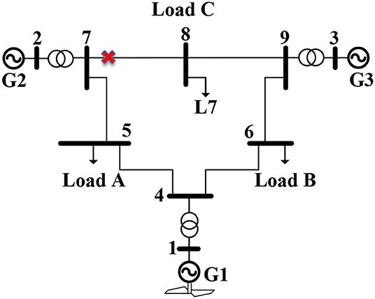
Figure 2. Modified IEEE 9 bus system.
A temporary three-phase short circuit to ground fault is applied to line 7–8. The wind turbine operates at three power factors (cosϕ): 0.9, 0.95, and 1.0. Figure 3A shows the reactive power produced by the wind farm. If the wind farm outputs more reactive power, the post-disturbance Bus 5 voltage will be recovered faster. Furthermore, more reactive power will flow through line 5–7 to the terminal bus of G2 (Figure 3C), which lifts the terminal bus voltage and increases the electromagnetic power output of G2. This improves G2 transient stability (Figure 3D). This observed behavior motivated the problem definition given in section The Combined Key Variable Identification and DT Designs.
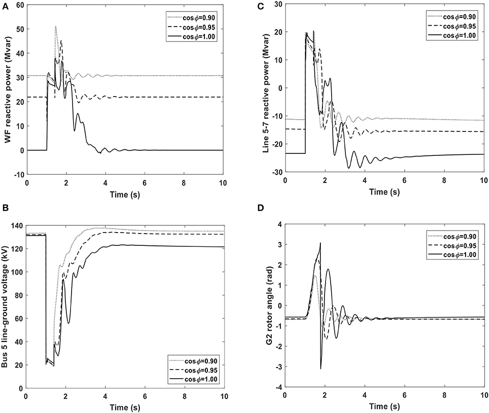
Figure 3. The influence of wind farm on rotor angle stability of G2. (A) Reactive power output of the wind farm. (B) Evolution of voltage magnitude at Bus 5. (C) Modification of reactive power transfer in line 5–7. (D) Collateral effect on the time response of the rotor angle of G2.
The Combined Key Variable Identification and DT Designs
Outline of the Proposed Method
This paper presents an approach that combines DTs and MVMO to select key variables and at the same time, to design DTs for transient stability estimation. Key variables refer to the variables that can unveil the influence of wind power and are also closely related to the transient behavior of synchronous generators. Taking key variables as the input, DTs are expected to be able to make a more accurate estimation of transient stability.
First, a group of key variables candidates are selected as DT inputs. Each of them is given a weight factor (which can be interpreted as a normalized score reflecting the degree of influence of the key variable on the resulting value of transient stability indicator). With the internal mapping function, MVMO mutates and hybridizes the new offspring of initial weight factors. Weight factors will change the key variable candidates' probability of being selected as the splitting property of DTs. Thus, DTs with different splitting rules are built. MVMO continuously evolves weight factors toward the direction of improving the DTs estimation accuracy, until a pre-defined convergence criterion (e.g., a given number of function evaluations) is met. At the end, a list of weight factors corresponding to the highest accuracy is obtained, and the variables with the largest weight factors are considered as the key variables. Meanwhile, DTs built using key variables and their weight factors as inputs are considered as the optimal performance trees, which will be used to estimate transient stability.
The flow chart of the proposed DTs and MVMO based approach is shown in Figure 4:
Step 1: First select a group of key variable candidates. This can be done based on existing operation experience or by considering all related variables to transient stability issues as candidates. Secondly, in order to make DTs reliably estimate transient stability, adequate training samples covering different operation conditions and faults scenarios are collected through off-line simulations or on-line measurements. Please note that depending on the studied power system model, different lengths of the time windows of the simulated/measured variable candidates might be needed. The time adaptive based approach proposed in Yu et al. (2018) is suggested as a good option to determine the length of the time windows.
Step 2: Initialize the weight factor for each key variable candidate. One combination of all weight factors is named as a particle.
Step 3: Build an ensemble of DTs to calculate the fitness for each particle.
Step 4: Judge if the termination criteria are satisfied. If yes, output a descending list of weight factors and optimal DTs; else, continue.
Step 5: MVMO mutates weight factors and generates new offspring. And then return to Step 3.
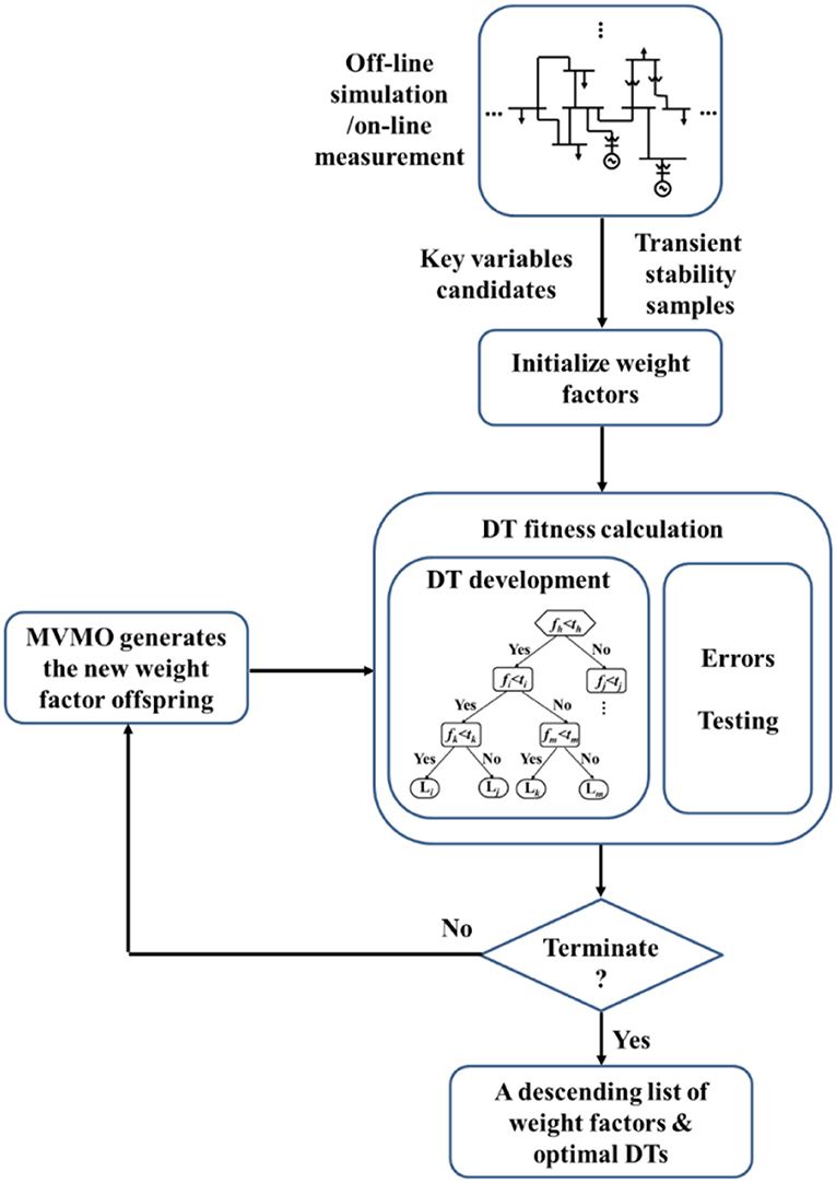
Figure 4. Key variables selection jointly using DTs and MVMO.
Mathematical Formulation of Involved Evolutionary Optimization
The evolution of weight factors can be defined by the following non-linear optimization:
subject to:
where x is a vector including L weight factors; and are the lower bound and the upper bound of the lth weight factor. Err(x) represents DTs estimation errors, which is defined as the sum of deviations between the estimated transient stability indicator ηDTs.k and the simulated one ηsim.k, associated to K tests, namely.
The ηsim.k is considered as the accurate value. Err(x) is minimized by using MVMO to continuously evolve weight factors.
Since transient stability mainly involves the relative motions of synchronous generator shafts, the stability indicator η is defined by (9) and described in detail in Powertech Labs Inc. (2011). It is worth pointing out that other indicators could be alternatively used in future studies.
where Δδ is the rotor angle difference between any two generators. If the maximum value of Δδ (namely maxΔδ) is less than an acceptable threshold Δδth, e.g., 180° (Kundur et al., 2004), the system is considered as transient stable. Conversely, the system is transient unstable.
In the interconnected power systems, transient stability means the ability of synchronous generators in one area to maintain synchronism against generators in other areas after a large disturbance. Under this condition, δ is redefined as the average rotor angle at the center of inertia of generators in one coherent area (Wang et al., 2016). When the angle difference between two coherent areas is <180°, that is to say, η is positive, the interconnected system is considered as transient stable.
Decision Trees (DTs)
DTs as intelligent classifiers have already been used to judge the transient stability status (stable or unstable) because of its good interpretability (or transparency) and easy implementation (Wehenkel et al., 1989; Amraee and Ranjbar, 2013; He et al., 2013; Guo and Milanović, 2014).
As shown in Figure 5, a decision tree is a graphical description of a well-defined decision problem, which is composed of a root node, branches, internal nodes and leaves (Gass and Harris, 1996; Rokach and Maimon, 2005). The root node is the starting point of a tree, without any incoming branch. A branch is a connection descending from an upper (parent) node to a lower (child) node. The internal nodes mean those nodes with incoming branches and outgoing branches. Each internal node splits its sample set into two or more sub-classes according to a certain splitting criterion. The nodes with incoming branches but without outgoing branches are called leaf nodes. Each leaf node is assigned a target value or a decision as its output. A decision tree is built in such a way that the training samples are recursively split into smaller left and right subsets in a top-down manner by selecting a certain splitting rule at a node until the stopping criterion is met.
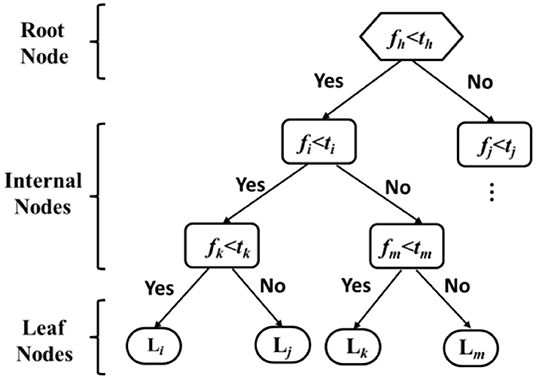
Figure 5. Typical structure of decision tree.
Essentially, a model built by DTs consists of a series of if-else splitting rules. How to select the splitting rules is critical for DTs to give satisfying estimation accuracy. One relative variance reduction based index is proposed in Ernst et al. (2005), namely:
where TS represents the training sample set at one node; LTS and RTS, respectively mean the left subset and the right subset which are obtained by splitting the parent training set TS. var(o|TS), var(o|LTS), and var(o|RTS) are the variances of output o in the training sets LS, LTS, and RTS. NTS, NLTS, and NRTS denote the sample numbers in three training sets.
This index quantifies the distance between the left subset and the right subset. The bigger it is, the larger the difference in η of samples in two subsets are, and the more possibly DTs classify a new observation to a group of samples with similar ηs. In this paper, this splitting index is further extended by multiplying a weight factor:
The Equation (11) is used to calculate a score for each possible splitting. The splitting with the largest score is adopted to split a TS into an LTS and an RTS. The bigger the weight factor is, the more possibly the corresponding variable is selected as the splitting attribute. A weight factor 0 means the relevant variable will not be considered during the selection of splitting attributes.
After building a group of DTs, the new observation will be navigated from a root node down to a leaf node, according to the if-else rule used at each node. The η average of samples in the leaf node is taken as approximately the estimation value for the new observation. Furthermore, the average of all DT estimations is considered as the definite estimation for the new observation, namely:
where η n is the estimation value made by the nth DT, and ηDTs is the average estimation given by a group of N DTs.
Mean–Variance Mapping Optimization (MVMO)
MVMO belongs to the family of population-based stochastic optimization. Its novel feature is the use of a special mapping function for mutating the new offspring, on the basis of the mean and variance of the n-best population attained so far. Due to its good performance in terms of convergence and quality of solutions, MVMO is used to reactive power management of offshore wind power plants (Theologi et al., 2017), reconfiguration of distribution systems (Rueda et al., 2015b), and identification of model parameters for real-time digital simulation (Gbadamosi et al., 2017).
The flow chart of MVMO is shown in Figure 6. In particular, MVMO is carried out as follows (Rueda et al., 2015a; Wildenhues et al., 2015):
Step 1: Initialize optimization parameters. Another significant feature of MVMO is that it normalizes variables xi to be optimized in the range of [0, 1] so that it ensures that no violation of the searching border occurs in mutated/hybridized offspring.
Step 2: Fitness evaluation. De-normalize each variable and calculate the value of fitness function.
Step 3: Termination judgment. Check if the termination criteria are satisfied. If yes, stop; if no continue.
Step 4: Archive/update the first n-best solutions in descending order of fitness value only if the new solutions are better than existing solutions. Furthermore, calculate the means, mapping shape for each variable xi.
Step 5: Parent assignment. Assign the best one or several solutions as the parents for mutating the offspring.
Step 6: Offspring generation. m variables in the parent vector are mutated by the following mapping function h, which is defined by the mean and the shape s1, s2.
The new value after mutation xr is calculated by:
The mapping curve is adjusted according to the progress of the search process in order to make MVMO continuously update the optimal solution candidates.
Step 7: The new offspring is sent back to Step 2. The above steps are repeatedly executed until a predefined termination criterion is fulfilled.
MVMO method provides a sequence of weight factors from the largest to the smallest. The system operator can decide how many variables are selected. Selecting more variables means more measurements and smaller estimation errors of decision trees. Selecting less variables means less measurements and larger errors of decision trees.
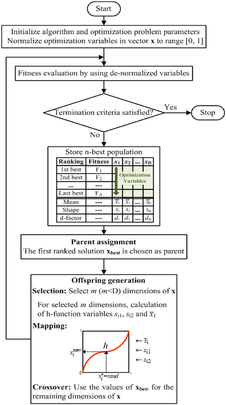
Figure 6. Flow chart of MVMO.
From Figure 4, when obtaining key variables (loop MVMO-build decision trees), a group of decision trees are built. For the sake of illustration, Figure 7 shows one part of a designed decision tree, taking the modified IEEE 9 bus system (indicated in section Illustration of the Influence of WT on Power System Transient Stability) as an example. Overall, it is worth pointing out that decision trees have rules that are built upon input-output data obtained from simulations of the power system. The rules constitute the knowledge extracted from the samples of inputs (e.g., generator speed S2, bus voltage magnitude V9 and V5, etc.) and output (stability indicator, e.g., rotor angle margin, which corresponds to the sampled inputs).
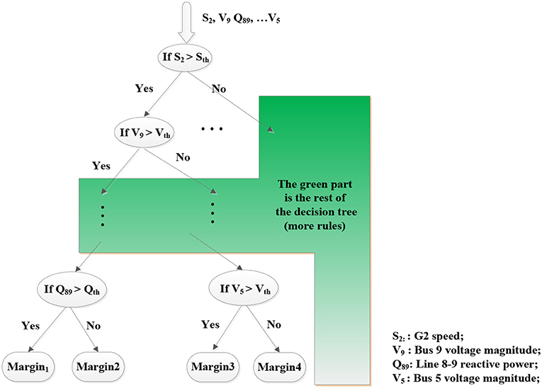
Figure 7. Illustration of decision trees.
Test Results on Ieee 9 Bus System
The proposed method is first illustrated on a variant of the IEEE 9-bus system, as shown in Figure 2. The parameters of the variant of the IEEE 9 bus system and the added wind turbines (developed on the basis of IEC 614000-27-1 standard) are given in Farrokhseresht et al. (2019). Interested reader can find details of the dynamic response of the wind turbine under different disturbances in Farrokhseresht et al. (2019). In order to build DTs, training samples are collected by considering the following uncertainties:
• Fault locations. A three-phase short circuit fault is applied on different locations [1, 50, 99%] in each of six transmission lines.
• Fault durations. Different fault durations are considered to simulate the severity of the fault.
• Inertia constant of G2. This factor determines how quickly G2 accelerates/decelerates due to the imbalance of electrical and mechanical torques.
In total, 396 samples (combinations of three samples of fault location in six transmission lines, 11 samples of fault duration, two samples of G2 inertia constant) are collected in PowerFactory 2016. The required amount of training samples depends on how many uncertainties should be investigated and the system size, which can be further refined by expert knowledge of system operators on network topology, critical faults, operation conditions, and so on.
A group of 58 variables that possibly influence G2 transient stability is selected as key variable candidates, which are listed in Table 1. The post-disturbance time responses of them are collected for DTs training and testing.
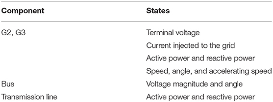
Table 1. Key variable candidates.
The involved algorithms of DTs, as well as MVMO, are programmed in Matlab 2016b. The settings of MVMO given in Rueda et al. (2015a) are also used in this paper. The parameters of DTs are given in Table 2. All variables in Table 1 are selected as the available properties to split a group of training samples. Therefore, 58 splitting attributes are used.

Table 2. Decision tree parameters.
The initial weight factor for each variable in Table 1 is 0.5. The upper bound of the weight factor is 1, and the lower bound is 0. 60 tests are generated to estimate the errors of DTs. Following the traditional practice in evolutionary algorithms, uniform random initialization is used. The optimized errors by MVMO after 200 iterations are shown in Figure 8. The better performance of MVMO was also observed when repeating the optimization 50 times. This is consistent with the observed computationally efficient performance (i.e., ability to quickly find a near-to-optimal solution within a very reduced computing budget, i.e., 200 iterations in the particular problem shown in this paper) of MVMO computationally expensive optimization problems as shown in Rueda et al. (2015a). A statistical assessment of the performance of MVMO and GA is out of the scope of this paper.
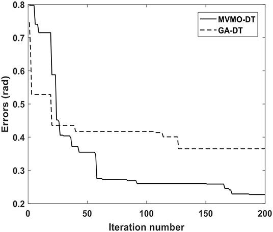
Figure 8. Evolution of DTs errors optimized by MVMO.
It is seen that by regulating the weight factors, DTs errors are reduced gradually. Table 3 gives the first eight biggest weight factors and two smallest weight factors in the list of weight factors which corresponds to the smallest error.
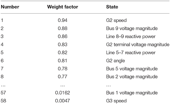
Table 3. Weight factors obtained on 9 bus system.
Among the first eight variables, the 1st and 6th variables are associated to the post-disturbance response of G2. They represent the influence of the fault on the generator motion dynamics. During the fault, the power balance at the G2 terminal bus is affected, which forces G2 to accelerate. After the fault, if G2 speed still is larger than the synchronous speed and the rotor angle exceeds the critical value, G2 loses transient stability.
The 5th and 7th variables represent the influence of wind farm reactive power on G2 transient stability, which is also illustrated in Figure 3. This shows the proposed method can effectively identify the key variables related to the influence of a wind farm. The 2nd and 3rd describe the reactive power support from G3 for the voltage at the load bus 8. These four variables together influence the terminal voltage of G2 (namely the 4th and 8th variables), and in this way, influence G2 active power output as well as its transient stability.
The first eight variables with the largest weight factors are selected as key variables. DTs taking them as the inputs give good estimations, as shown in Figure 9A. Next, a natural question to be answered is: using eight key variables, could DTs achieve a similar estimation accuracy like using all 58 variables? The estimation errors obtained by using all 58 variables and by using the eight key variables are compared in Figure 9B. It is seen that the estimations made by using eight variables (blue circles) have nearly the same accuracy as the estimations done by using 58 variables (black diamonds).
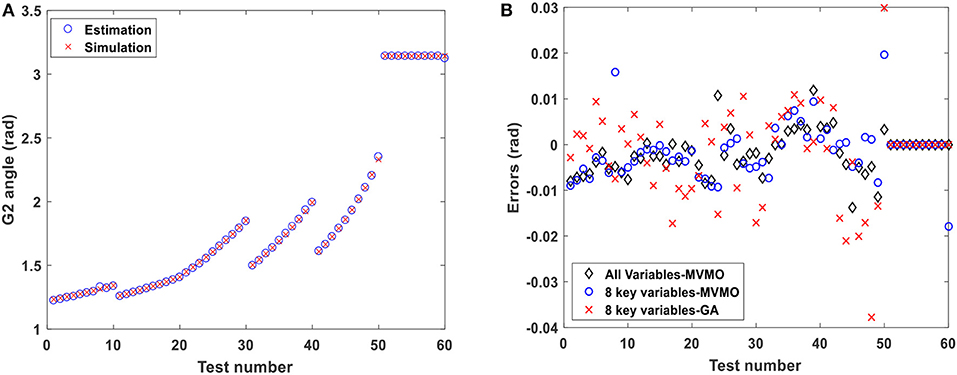
Figure 9. (A) Estimation using 8 variables; (B) Errors using different amounts of variables and different methods.
In order to verify the efficiency of MVMO, a Genetic Algorithm with a Multi-Parent Crossover is adopted to optimize weight factors (Elsayed et al., 2014). The parameters of this algorithm, as given in Elsayed et al. (2014) are used also in this paper. Its convergence during 200 iterations is shown in Figure 8. It can be seen that MVMO finds faster the weight factors which bring forth the less estimation errors of DTs. Respectively using the optimal weight factors searched by GA and MVMO to build DTs, the estimation errors of 60 tests are shown in Figure 9B. It can be seen that DTs using the key variables selected by MVMO (blue circles) give less estimation errors.
Test Results On Great Britain (GB) System
Key Variable Identification
The proposed method is further tested on a reduced size model of the Great Britain (GB) system in Figure 10. The GB system has three sub-areas, the north, the center, and the south, which consists of 29 power plants, 161 buses, 119 lines. The parameters of the reduced size model of the GB system and the added wind turbines (developed on the basis of IEC 614000-27-1 standard) are given in Farrokhseresht et al. (2019). Considering the complexity of the GB system, the proposed method is applied to a three-phase short circuit to a ground fault between the north and the center, which causes the generators in the north area to lose transient stability.
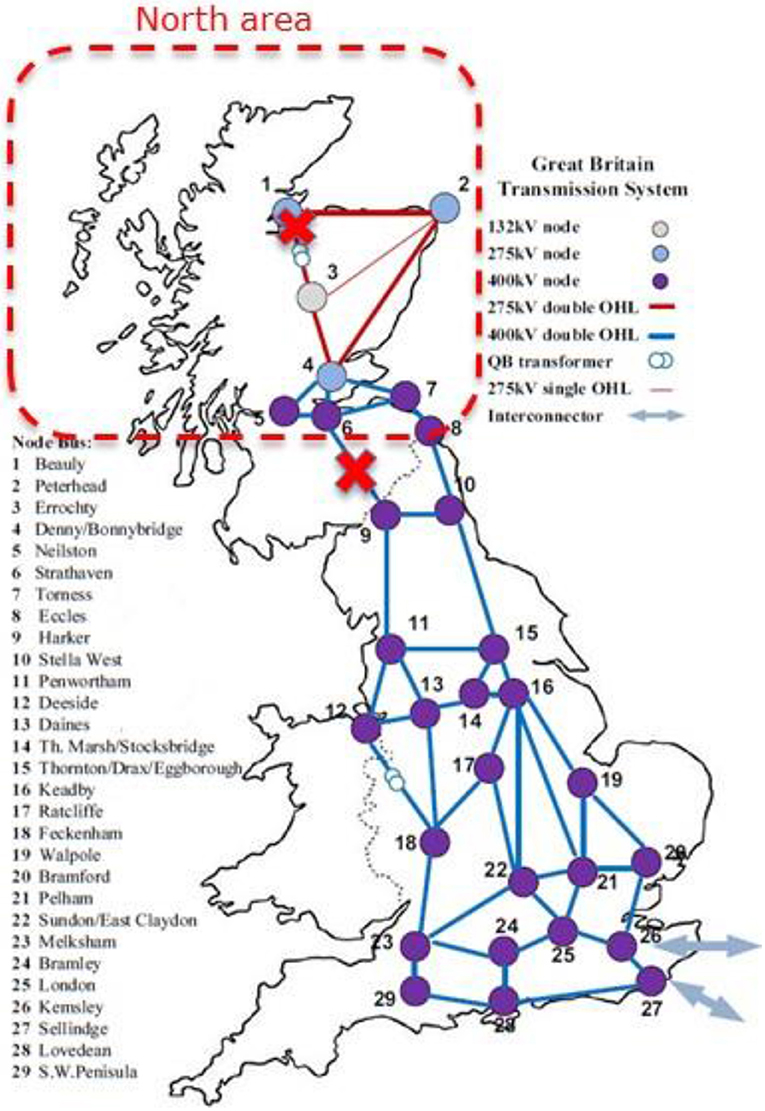
Figure 10. GB test system.
In this case, more wind penetration levels, different dispatches between synchronous generators and wind farms are further considered. The following uncertainties are investigated to cover different operation conditions for DTs training.
• Fault duration. Indeed, GB system is fairly (rotor angle) stable for large-disturbances. So in order to generate unstable samples, the fault duration is perturbed in a range from 0.2 to 0.3 s.
• Dispatches among synchronous generators. In the north area, synchronous generators are distributed in 4 zones. Different dispatching scenarios between them are generated. Moreover, because of the change of commissioned generator units, the inertia of different zones is also changed.
• Wind penetration levels in the north area. The initial output of synchronous generators and wind turbines are listed in Table 4.
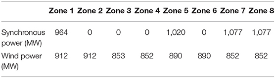
Table 4. Synchronous power and wind power.
One part of synchronous generators in Table 4 is further decommissioned and replaced by wind generators in order to analyze transient stability under high wind power penetration levels. The wind penetration levels dealt with in this test case are listed in Table 5.

Table 5. Wind penetration levels.
In total, 633 samples are collected. For each of them, 98 key variable candidates in Table 6 are observed.
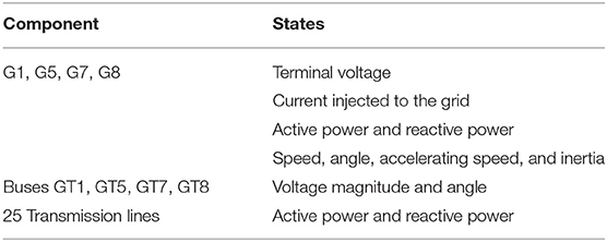
Table 6. Observed variables in the north area.
Similar to test case 1, 100 decision trees (cf. Table 7) are built. In each tree, one leaf node only includes one sample. Each variable in Table 6 is selected as a property to split a group of training samples. Therefore, 98 splitting attributes are available.

Table 7. Decision tree parameters.
An initial weight factor, 0.5, is given to each variable. It's upper bound and the low bound are respectively 1 and 0. The convergence of MVMO optimization process in 1,000 iterations is depicted in Figure 11.
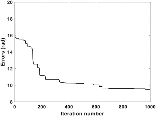
Figure 11. Evolution of DT errors optimized by MVMO in GB system.
It takes nearly 5 h to finish these 1,000 iterations by using a parallel computing process on a computer with Intel(R) Core(TM) i7-8650U 2.11 GHz. To tackle changes in operating conditions of a power system, updating the DTs and weighting factors will be needed. To this aim, the computation time can be lowered by extending the proposed approach with the distributed computing strategy defined in He et al. (2013). Table 8 gives the selected 10 key variables from the weight factor list corresponding to the minimum error. It is seen in Table 8 that the transient stability of zone 1 is influenced by:
• The loading level of generators in zone 1, which are determined by the terminal bus voltage (variable 1) and the current injected into the grid (variable 3). A higher loading level after the disturbance will impose one bigger electromagnetic torque and preventing the rotor angle from increasing.
• The generator speed (namely variable 5), which represents the obtained accelerating energy during the fault.
• The reactive power distribution after the fault, namely the 2nd, 4th, 10th, and 11th variables. They jointly influence the voltage at the terminal bus connecting the generators in zone 1. It is known that a too low terminal voltage will prevent generators from outputting normally active power and force the rotors to accelerate.
• The active power flow, namely the 6th, 7th, 8th, and 9th variables. These values influence directly the power balance on the rotor and transient stability.
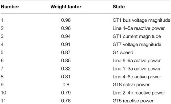
Table 8. Selected key variables in GB system.
Transient Stability Assessment
Next, DTs are built using the above 11 key variables, and the estimation accuracy is tested under different operating scenarios.
65% Wind Penetration
The comparison between using 11 key variables and 98 available variables is made in Figure 12. It can be seen that the estimations done by using 11 key variables provide a similar accuracy as using 98 variables.
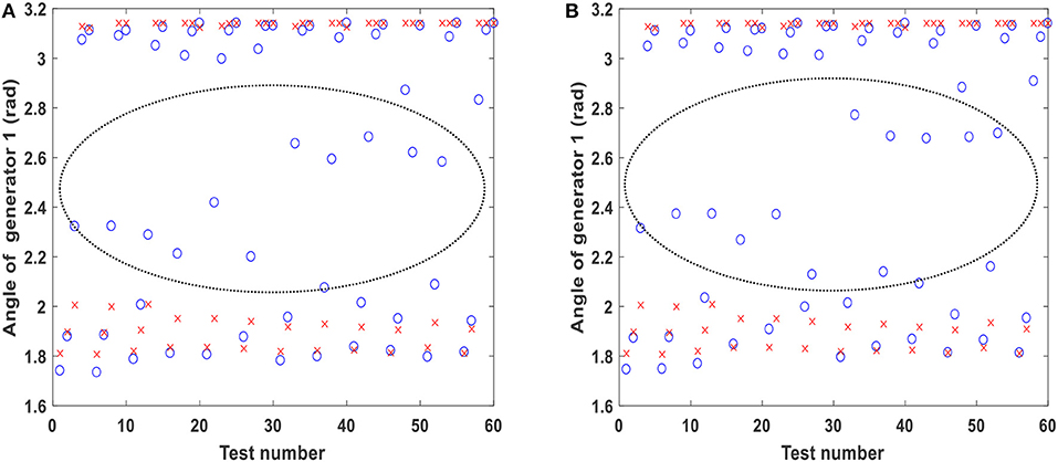
Figure 12. (A) Results with 98 variables; (B) Results with 11 key variables under 65% wind penetration. O = Estimation; X = Simulation.
Another point which is noticed in Figure 12 is that there are some points with relatively large estimation errors, circled by the dashed oval. This is caused by the sudden transition from transient stability to transient instability due to a minor change of fault duration, which is shown in Figure 13. Under the condition that other uncertainties considered in section Key Variable Identification are neglected, a slight perturbation on the fault duration from 0.271 to 0.272 s causes transient instability. During the transition (border) from stability to instability, usually, the artificial intelligence-based methods have relatively large errors.
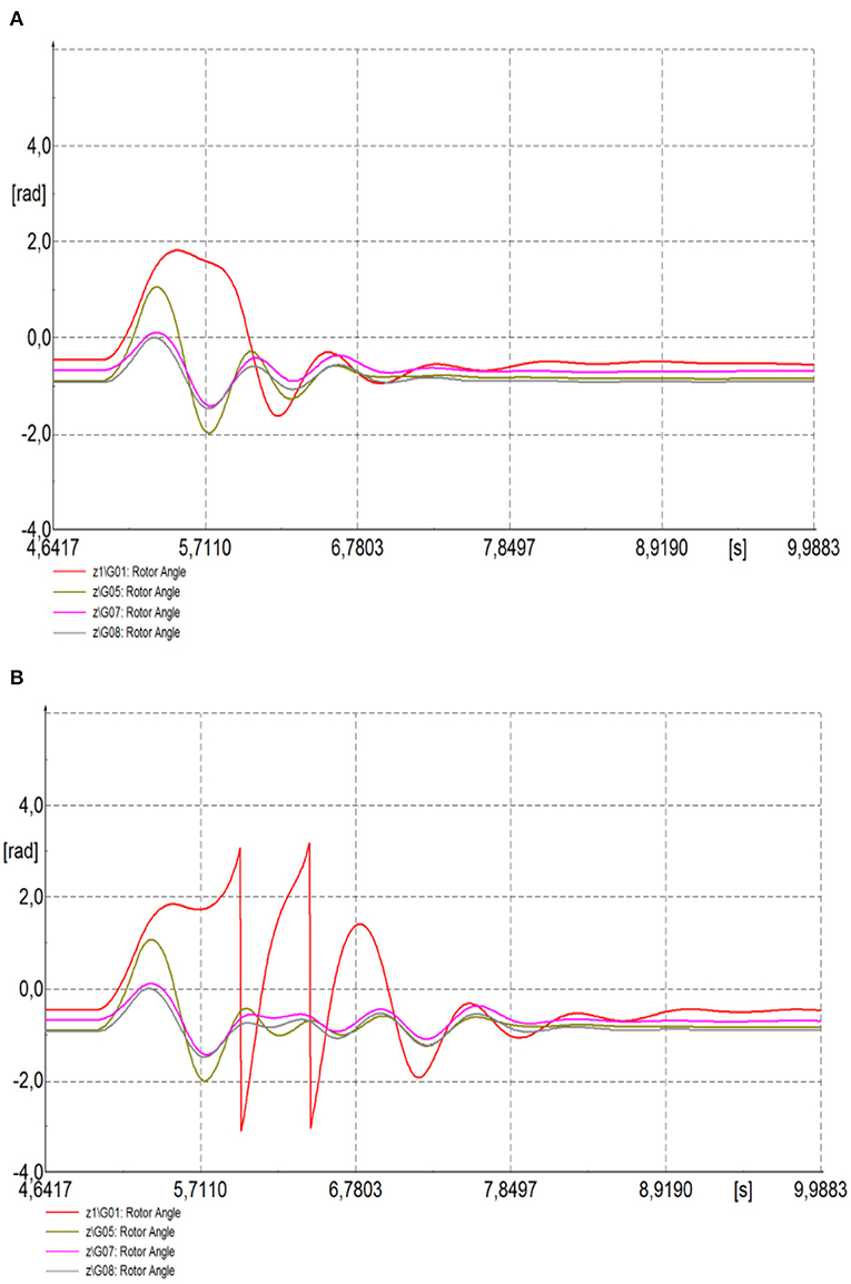
Figure 13. G1 angle: (A) fault duration of 0.271 s; (B) fault duration of 0.272 s.
70% Wind Penetration
Forty-six tests are made at this penetration level, which cover different fault duration and dispatching scenarios. The results are shown in Figure 14. It can be seen again that the estimation done by using 11 key variables gets the same accuracy as the estimation done using all variables. DTs give good estimations for stable cases and unstable cases (upper and lower points in Figure 14).
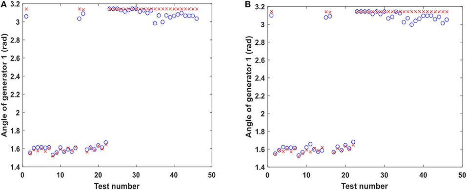
Figure 14. (A) Results with 98 variables; (B) Results with 11 key variables under 70% wind penetration. O = Estimation; X = Simulation.
79% Wind Penetration
At the end, more synchronous generators are decommissioned and wind penetration nearly reaches 80% in the north area. For all used 48 tests, transient instability occurs. Figure 15 demonstrates that using all variables and using 11 key variables, both provide good and similar estimations.
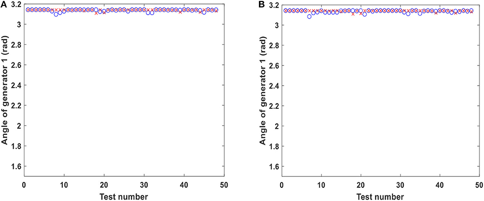
Figure 15. (A) Results with 98 variables; (B) Results with 11 key variables under 79% wind penetration. O = Estimation; X = Simulation.
Implementation of the Proposed Approach
The typical way of using DTs (at the top half of Figure 16) is to first select manually a group of variables of interest for transient stability. Then the rules for splitting samples are figured out and DTs are built. The performance of DTs is tested, and, correspondingly, the researcher decides whether or not to adjust the splitting rules. If yes, the new rules are sent to DTs and new trees are built. Similarly, the performance of new trees is tested and this procedure is repeated until the performance of DTs is satisfactory.
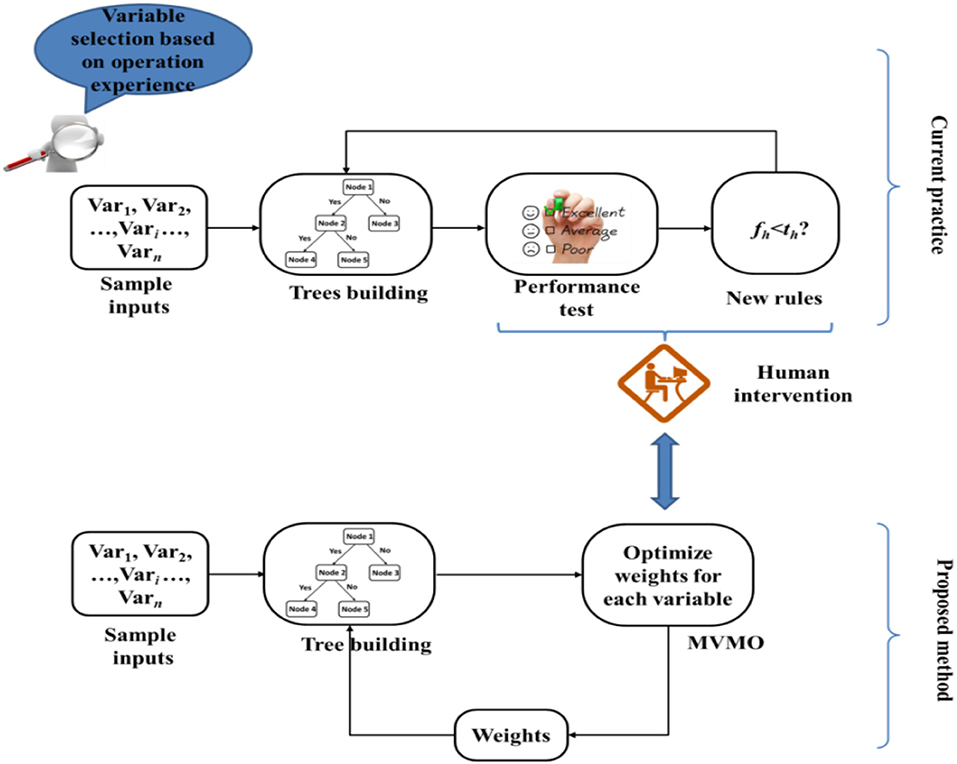
Figure 16. Comparison between proposed method and current practice.
Compared with the above method, the selection of key variables and the training of DTs are done at the same time and automatically by using MVMO in the proposed method, as shown by the bottom half in Figure 16. The users can input any variables which they want to investigate, together with initial weight factors in the range [0, 1]. MVMO is responsible to mutate/optimize weight factors. The new weight factors are sent back to DTs to evaluate the fitness. In this way, MVMO continues to automatically optimize weight factors until the stopping criterion is satisfied.
On the basis of the obtained weight factors, system operators can select the first n variables with the largest weight factors as the key variables. The value of n is decided by the estimation accuracy, which can be accepted by system operators. Selecting more variables means more installations of measurement devices and smaller estimation errors of DTs. Inversely, selecting less variables means less measurements and larger DTs' estimation errors.
At the same time, DTs built using n key variables are considered as the finally trained trees for transient stability assessment. One possible application is demonstrated in Figure 17. First, considering the large scale and the complexity of real power systems, different groups of DTs are trained off-line and separately for different fault scenarios. In practice, when a fault occurs, a disturbance indicator will send the fault information to a classifier. This classifier is responsible to select the corresponding group of DTs, like group 1. Measurement devices (like PMU) collect the post-disturbance values of key values. Taking this information as the input, DTs will estimate stability indicator, like Margin η1.
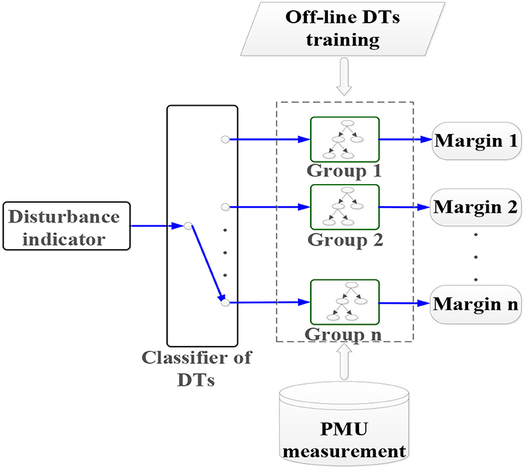
Figure 17. Demonstration of applying DTs.
Conclusions
This paper proposed a DTs and MVMO based method to identify key variables and to estimate transient stability in power systems with high penetration of wind power. Key variables are defined as the variables which are related to the transient stability performance of a power system. Usually, the selection of key variables relies on system operators' expert knowledge and attentive investigation on possible transient instability. Here, such a selection is made through optimizing DTs estimation errors by MVMO, with the help of a weight factor assigned to each key variable candidate. The optimized weight factors indicate key variables, and at the same time, DTs built using key variables are considered as the optimal performance trees for transient stability estimation.
The test results on the 9-bus system and GB system show that the proposed method not only identified the key variables related to the influence of wind farms but also find other key variables that conform to the generic understanding on transient stability. In most tests, DTs built using key variables give nearly accurate estimations as those built using all available variables. This shows that the proposed method can select correctly a few of key variables to reduce measurement/communication investment, and at the same time keep good estimation accuracy for transient stability.
Another finding from the obtained results is that in some transitions from transient stability to transient instability due to slight parameter changes, DTs may have some relatively large errors. This is a common challenge for artificial intelligence-based methods. More research effort should be put into solving the misjudgement on the border between stability and instability. Moreover, to apply this proposed method in real power systems, it is necessary to collect adequate samplings on possible operating conditions and fault scenarios, which is quite difficult due to the complexity of real systems. A promising solution is to apply the proposed method to typical operating conditions and critical fault scenarios. This study is currently being extended to consider other factors that also affect transient stability of power systems with high penetration of power electronic interfaced generation. Among these factors are the variable number of wind power generators in service and the degree of randomness of the active power output of wind power generators. A detailed comparison with other options with data mining based algorithms or other forms of decision trees, e.g., like algorithms presented in Kamwa et al. (2010) and Rahmatian et al. (2017), is a topic for future research after this paper. Future work should also be performed to provide a comparative assessment of using other optimization tools and by using real-time data (which can be generated by using a digital twin of a real system built in a real-time digital simulator). Such comparison shall include a detailed comparative analysis with statistical tests.
Data Availability Statement
The datasets for this article are not publicly available due to confidentiality agreements within the MIGRATE H2020 project (https://www.h2020-migrate.eu/). Specific questions on figures and tables should be directed to the corresponding author (José L. Rueda Torres, j.l.ruedatorres@tudelft.nl).
Author Contributions
All authors listed have made a substantial, direct and intellectual contribution to the work, and approved it for publication.
Conflict of Interest
The authors declare that the research was conducted in the absence of any commercial or financial relationships that could be construed as a potential conflict of interest.
Acknowledgments
This project has received the funding from the European Union's Horizon 2020 research and innovation programme under grant agreement No. 691800. This paper reflects only the authors' views and the European Commission is not responsible for any use that may be made of the information it contains.

References
Amraee, T., and Ranjbar, S. (2013). Transient instability prediction using decision tree technique. IEEE Trans. Power Syst. 28, 3028–3027. doi: 10.1109/TPWRS.2013.2238684
Cepeda, J. C., Rueda, J. L., Colomé, D. G., and Echeverría, D. E. (2014). Real-time transient stability assessment based on centre-of-inertia estimation from phasor measurement unit records. IET Gen. Transm. Distrib. 8, 1363–1376. doi: 10.1049/iet-gtd.2013.0616
Cirrincione, M., Pucci, M., and Vitale, G. (2015). Neural MPPT of variable-pitch wind generators with induction machines in a wide wind speed range. IEEE Trans. Ind. Appl. 49, 942–953. doi: 10.1109/TIA.2013.2242817
Elsayed, S. M., Sarker, R. A., and Essam, D. L. (2014). A new genetic algorithm for solving optimization problems. Eng. Appl. Artif. Intell. 27, 57–69. doi: 10.1016/j.engappai.2013.09.013
Ernst, D., Geurts, P., and Wehenkel, L. (2005). Tree-based batch mode reinforcement learning. J. Mach. Learn. Res. 66, 503–556. doi: 10.5555/1046920.1088690
Faried, S. O., Billinton, R., and Aboreshaid, S. (2010). Probabilistic evaluation of transient stability of a power system incorporating wind farms. IET Renew. Power Gener. 4, 299–307. doi: 10.1049/iet-rpg.2009.0031
Farrokhseresht, N., van der Meer, A. A., Rueda Torres, J. L., van der Meijden, M. A. M. M., and Peter Palensky, A. D. (2019). “Increasing the share of wind power by sensitivity analysis based transient stability assessment,” in 2nd International Conference on Smart Grid and Renewable Energy (Doha).
Gass, S. I., and Harris, C. M. (1996). Encyclopedia of Operations Research and Management Science. Hingham, MA: Kluwer Academic Publishers.
Gbadamosi, A., Rueda, J. L., Wang, D., and Palensky, P. (2017). “Application of mean-variance mapping optimization for parameter identification in real-time digital simulation,” in 2017 Federated Conference on Computer Science and Information Systems (FedCSIS) (Prague), 11–16.
Guo, T., and Milanović, J. V. (2014). Probabilistic framework for assessing the accuracy of data mining tool for online prediction of transient stability. IEEE Trans. Power Syst. 29, 377–385. doi: 10.1109/TPWRS.2013.2281118
He, M., Zhang, J. S., and Vittal, V. (2013). Robust online dynamic security assessment using adaptive ensemble decision-tree learning. IEEE Trans. Power Syst. 28, 4089–4098. doi: 10.1109/TPWRS.2013.2266617
Hoballah, A., and Erlich, I. (2012). Online market-based rescheduling strategy to enhance power system stability. IET Gen. Transm. Distrib. 6, 30–38. doi: 10.1049/iet-gtd.2011.0265
Huang, C., Li, X. F., and Jin, Z. Q. (2015). Maximum power point tracking strategy for large-scale wind generation systems considering wind turbine dynamics. IEEE Trans. Ind. Electron. 62, 2530–2539. doi: 10.1109/TIE.2015.2395384
Kamwa, I., Samantaray, S. R., and Joos, G. (2010). Catastrophe predictors from ensemble decision-tree learning of wide-area severity indices. IEEE Trans. Smart Grid 1, 144–158. doi: 10.1109/TSG.2010.2052935
Krause, P. C., Wasynczuk, O., and Pekarek, S. (2012). Electromechanical Motion Devices. New York, NY: Wiley-IEEE Press.
Kundur, P., Paserba, J., Ajjarapu, V., Andersson, G., Bose, A., Canizares, C., et al. (2004). Definition and classification of power system stability IEEE/CIGRE joint task force on stability terms and definitions. IEEE Trans. Power Syst. 19, 1387–1401. doi: 10.1109/TPWRS.2004.825981
Lin, L., Zhao, H. L., Lan, T., Wang, Q., and Zeng, J. (2013). Transient Stability Mechanism of DFIG Wind Farm and Grid-Connected Power System. Grenoble: PowerTech.
Liu, S. W., Li, G. Y., and Zhou, M. (2016). Power system transient stability analysis with integration of DFIGs based on centre of inertia. CSEE J. Power Energy Syst. 2, 20–29. doi: 10.17775/CSEEJPES.2016.00018
Meegahapola, L., Flynn, D., and Littler, T. (2008). “Transient stability analysis of a power system with high wind penetration,” in Universities Power Engineering Conference (Padova).
Oluic, M., Ghandhari, M., and Berggren, B. (2017). Methodology for rotor angle transient stability assessment in parameter space. IEEE Trans. Power Syst. 32, 1202–1211. doi: 10.1109/PESGM.2017.8274261
Powertech Labs Inc. (2011). TSAT Transient Security Assessment Tool–User Manual. Available online at: https://eva.fing.edu.uy/pluginfile.php/71802/mod_resource/content/1/TSAT_User_Manual.pdf
Rahmatian, M., Chen, Y. C., Palizban, A., Moshref, A., and Dunford, W. G. (2017). Transient stability assessment via decision trees and multivariate adaptive regression splines. Electric Power Syst. Res. 142, 320–328. doi: 10.1016/j.epsr.2016.09.030
Rokach, L., and Maimon, O. Z. (2005). Data Mining and Knowledge Discovery Handbook. Boston, MA: Springer.
Rueda, J. L., Cepeda, J., Erlich, I., Echeverría, D., and Argüello, G. (2015a). Heuristic optimization based approach for identification of power system dynamic equivalents. Int. J. Electric. Power Energy Syst. 64, 185–193. doi: 10.1016/j.ijepes.2014.07.012
Rueda, J. L., Loor, R., and Erlich, I. (2015b). “MVMO for optimal reconfiguration in smart distribution systems,” in Proceedings of 9th IFAC Symposium on Control of Power and Energy Systems (New Delhi), 1–6. doi: 10.1016/j.ifacol.2015.12.390
Shewarega, F., Erlich, I., and Rueda, J. L. (2009). “Impact of large offshore wind farms on power system transient stability,” in Power Systems Conference and Exposition (Seattle, WA).
Shi, L. B., Sun, S. M., Yao, Z. L., Ni, Y., and Bazargan, M. (2014). Effects of wind generation intermittency and volatility on power system transient stability. IET Renew. Power Gener. 8, 509–521. doi: 10.1049/iet-rpg.2013.0028
Theologi, A. M., Ndreko, M., Rueda, J. L., van der Meijden, M. A. M. M., and González-Longatt, F. (2017). “Optimal management of reactive power sources in far-offshore wind power plants,” in 2017 IEEE Manchester (Manchester: PowerTech), 1–6.
Velez, F. G., Centeno, V. A., and Phadke, A. G. (2017). “Multiple swing transient stability assessment with phasor measurements,” in Proceedings of 2017 IEEE (Manchester: PowerTech). doi: 10.1109/PTC.2017.7981173
Vu, T. L., and Turitsyn, K. (2016). Lyapunov functions family approach to transient stability assessment. IEEE Trans. Power Syst. 31, 1269–1277. doi: 10.1109/TPWRS.2015.2425885
Wang, B., Fang, B., Wang, Y., Liu, H., and Liu, Y. (2016). Power system transient stability assessment based on big data and the core vector machine. IEEE Trans. Smart Grid 7, 2561–2569. doi: 10.1109/TSG.2016.2549063
Wehenkel, L., Van Cutsem, T., and Ribbens-Pavella, M. (1989). An artificial intelligence framework for on-line transient stability assessment of power systems. IEEE Trans. Power Syst. 4, 789–800. doi: 10.1109/59.193853
Wildenhues, S., Rueda, J. L., and Erlich, I. (2015). Optimal allocation and sizing of dynamic var sources using heuristic optimization. IEEE Trans. Power Syst. 30, 2538–2546. doi: 10.1109/TPWRS.2014.2361153
Keywords: transient stability, decision trees (DTs), mean–variance mapping optimization (MVMO), wind power, massive InteGRATion of power electronic devices (MIGRATE)
Citation: Wang D, Rueda Torres JL, Rakhshani E and van der Meijden M (2020) MVMO-Based Identification of Key Input Variables and Design of Decision Trees for Transient Stability Assessment in Power Systems With High Penetration Levels of Wind Power. Front. Energy Res. 8:41. doi: 10.3389/fenrg.2020.00041
Received: 30 November 2019; Accepted: 28 February 2020;
Published: 19 March 2020.
Edited by:
Francisco Gonzalez-Longatt, University of South-Eastern Norway, NorwayReviewed by:
Mohd Zamri Che Wanik, Qatar Foundation, QatarAyman Hoballah, Tanta University, Egypt
Worawat Nakawiro, King Mongkut's Institute of Technology Ladkrabang, Thailand
Copyright © 2020 Wang, Rueda Torres, Rakhshani and van der Meijden. This is an open-access article distributed under the terms of the Creative Commons Attribution License (CC BY). The use, distribution or reproduction in other forums is permitted, provided the original author(s) and the copyright owner(s) are credited and that the original publication in this journal is cited, in accordance with accepted academic practice. No use, distribution or reproduction is permitted which does not comply with these terms.
*Correspondence: José L. Rueda Torres, j.l.ruedatorres@tudelft.nl