Research on the data-driven inter-well fracture channeling identification method for shale gas reservoirs
 Feng He
 Ming Yue
  Wei Jiang
 Chao Qian
- Shale Gas Exploration and Development Department, CNPC Chuanqing Drilling Engineering Co., Ltd., Chengdu, China
The issue of inter-well fracture channeling in shale reservoirs is becoming increasingly prominent, significantly impacting the production of nearby wells. Therefore, it is crucial to accurately determine the location of fracture channeling in order to effectively design anti-channeling measures and optimize reservoir fracturing. In this paper, a data-driven fracture propagation model and fracture channeling identification method are established. In the model, the fracture morphology is fitted by the bottom-hole flowing pressure constraint. The bottom-hole flowing pressure (pwp) calculated by the construction pump pressure and the fluid wellbore flow is mainly considered as the real solution. The bottom-hole flowing pressure (pwf) calculated by the construction displacement and the fracture morphology is used as the constraint variable, and the fracture parameters are changed using the SPSA optimization algorithm to realize the dynamic fitting of the fracture morphology. In order to accurately describe the position of fracture channeling, the seepage radius of the fracture boundary is introduced to calculate the volume of fracture reconstruction. The volume coefficient of repeated reconstruction is used as the quantitative evaluation index of fracture channeling. This approach enables an accurate depiction of the position of fracture channeling. Finally, the model method is applied to the actual fracture channeling well. The study shows that the fracture length of the well inversion is greater than the well spacing, and there is a possibility of inter-well fracture channeling. The volume coefficient of repeated reconstruction is 8%, similar to the critical fracture channeling index. There are nine fracturing sections with fracture channeling, and the maximum fracture channeling coefficient is 14.2%. This paper successfully explains the reason for cross-well fracture channeling, and its conclusion aligns with the actual monitoring results. The proposed method in this paper effectively identifies the location of fracture channeling and offers guidance for optimizing channeling prevention in subsequent designs.
1 Introduction
Fracturing is a crucial technology for the commercial development of shale reservoirs (Wang et al., 2012; Du et al., 2014; Huang et al., 2022). However, the fracturing of infill wells in the later stage can often result in fracture communication between new and old wells, leading to fracture channeling. This communication issue significantly impacts the production of parent or adjacent wells, causing substantial economic losses (He et al., 2020). Hence, there is an urgent need to implement new technologies that enable the quantitative identification of reservoir inter-well fracture channeling.
The current methods for identifying fracture channeling can be categorized into three types: microseismic monitoring technology, tracer monitoring technology, and the dynamic analysis method (Zhang et al., 2019; Zhao B. et al., 2020; Fu and Dehghanpour, 2020; Escobar et al., 2021). Microseismic monitoring technology is a crucial tool used in oilfield exploration and development processes. It involves locating fractures by detecting induced microseismic events that occur during fracturing. This method is primarily used for dynamically imaging fracturing fractures in low-permeability reservoirs, enabling the tracking of the fracturing range and providing an objective evaluation of the location of fracture channeling (Zhang et al., 2019). Aleksandrov et al. (2018) and Wu et al. (2017) used this method for fracture analysis. However, with the advancement of technology, it has been found that the error of microseismic monitoring technology is large, and the actual fractures are only between 30% and 70% of the monitoring results (Huang et al., 2021a). The credibility of evaluating fracture channeling using microseismic monitoring can be greatly reduced. Tracer monitoring technology is a direct method for determining reservoir communication (Meng et al., 2022). This method reflects the flow of reservoir fluid and inter-well communication information through the breakthrough curve of tracer concentration monitored in the production well. Brigham and Smith (1965) were the first to apply chemical tracers to the evaluation of reservoir fracturing and achieved positive results. Over time, the types of tracers have become more diverse, allowing for the evaluation of various pieces of information, such as fracture type, reservoir seepage capacity, and fracture channeling (Geng et al., 2017). However, tracer monitoring technology is time-consuming and requires a long cycle to draw the tracer concentration curve. Additionally, the economic cost of using tracers is high. As a result, this method is less commonly used in the evaluation of inter-well fracture channeling. Instead, the dynamic analysis method relies on the dynamic data of production wells or fracturing wells to analyze the degree of fracture channeling. This includes examining the changes in parent-well productivity and child-well construction pressure (Puneet et al., 2021). Ajani and Kelkar (2012) used the productivity change of the parent well to evaluate the influence of the well spacing and the production time of the parent well on fracture channeling and provided a reference for the well location deployment. King et al. (2017) analyzed the influence of fracturing parameters on fracture channeling according to the change in child-well construction pressure. With the advantages of low cost and simple operation, the dynamic analysis method is widely used in the analysis of inter-well fracture channeling. However, this method also has the disadvantage of being time-consuming and being affected by multi-well interference and external factors, resulting in a large analysis error. Furthermore, all three methods mentioned above are qualitative evaluations of fracture channeling, which cannot accurately determine the location of fracture channeling or propose specific solutions to address this phenomenon. The main cause of inter-well fracture channeling is the dominant fracture channel formed by child-well fracturing to connect with the fractures of the parent well. Therefore, the most effective approach to determine the position of pressure channeling is to accurately describe the fracture morphology and quantitatively identify the fracture communication position.
The simulation methods of fracture propagation are mainly divided into the finite element method (FEM), extended finite element method (XFEM), boundary element method (BEM), and unconventional fracture propagation model (UFM) (Li and Wang, 2005; Olson, 2008; Zhou et al., 2020; Huang et al., 2021b). Dali Taleghani (2010) used the XFEM to simulate the fracture propagation of hydraulic fracturing vertical wells in shale reservoirs. The BEM can transform the problem into a boundary integral equation, and the approximate solution can be found discretely on the boundary. The BEM is more suitable for cases with a complex fracture network, but its applicability in simulating fluid–solid coupling problems is poor (Olson, 2008). The UFM adopts the 2D displacement discontinuity method to solve the interaction between reservoir stress field and fractures. Meanwhile, the fracture width and proppant concentration can be calculated using a 3D fracture height equation and proppant sedimentation equation (Weng et al., 2011; Kresse and Weng, 2018). However, these types of fracture propagation simulation methods have their own advantages in solving the calculation of fracture parameters and reservoir stress parameters, but the fracture morphology described is mostly a single fracture. The fractures in the reservoir are mostly staggered branch fractures, and fracture channeling is also formed by the intersection of fracture branches. Therefore, a single fracture cannot effectively describe the channeling fracture. Zhao et al. (2021), Zhao H. et al. (2020), and Sheng et al. (2023) proposed a reservoir fracturing model based on lightning simulation, which can simulate the fracture morphology of complex induced fractures. In this paper, the method proposed by Zhao H. et al. (2020) is used to establish a fracture channeling identification model based on the connection element method. In the method, the fluid flow in the wellbore and fracture is considered, and the fracture boundary seepage radius is introduced to calculate the fracture reconstruction volume. Taking the volume coefficient of repeated stimulation as the quantitative evaluation index of fracture channeling, the accurate description of the location of fracture channeling is realized, and it is analyzed and applied in the actual fracture channeling wells.
2 Mathematical model of shale reservoir channeling identification based on the connection element method
2.1 Fracture propagation model based on the connection element method
In order to simulate accurately and quickly, we simplify the reservoir and use the connection element method to characterize the reservoir model. In the model, the reservoir and rock are discretized into continuous connection nodes, and the communication relationship between the nodes and the adjacent nodes is established by a connection, as shown in Figure 1. In the acquisition of connection unit data, the reservoir is first divided into unevenly distributed grids according to the geological model, and the center of each grid is considered the initial node. The initial node parameters are obtained from the actual geological model obtained using the interpolation algorithm. In the simulation process, the nodes can be increased or decreased. Second, when the special medium (such as natural fractures) is distributed into the reservoir, a new node is added to describe the special lithology medium. On the basis of the node connection system, flexible meshless nodes can be used to replace the traditional mesh topology. Figure 1 shows that the blue to green nodes represent reservoir nodes of different parameters, and the red nodes represent fracture nodes.
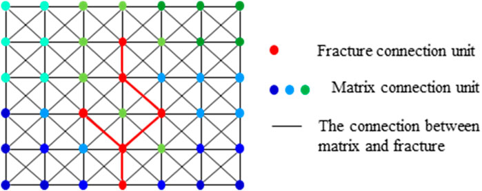
FIGURE 1. Reservoir and fracture node division of the connection element method.
2.1.1 Mechanical model of fractures
In the model, considering that the rock is a porous elastic medium, the principal stress parameters of the rock can be obtained by combining the logging data, which are expressed as
where σh represents the minimum horizontal principal stress, MPa; σH represents the maximum horizontal principal stress, MPa; αvert and αhor represent the vertical and horizontal Biot coefficient; ξH and ξh represent the strain coefficient of the maximum principal stress and the minimum principal stress, respectively; ν represents Poisson‘s ratio; E represents the elastic modulus, GPa; and Pp represents the pore pressure, MPa. In this paper, it is considered that rock fracturing is affected by opening and shearing, which is I–II composite fractures (Feng and Kang, 2013). Rock failure is affected by the combined action of horizontal principal stress σh, σH, and fluid pressure in the fracture, as shown in Figure 2A. According to the superposition principle, the composite model can be decomposed into two independent models. Figure 2B shows that the fracture is subjected to far-field stress; Figure 2C shows that the fracture is affected by the fluid pressure in the fracture.
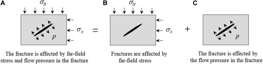
FIGURE 2. Fracture stress decomposition.
For model (b), the stress intensity factor at the crack tip is expressed as
For model (c), the stress intensity factor at the fracture tip is expressed as
After superposition, the final stress intensity factor at the fracture tip can be obtained. Since the pressure in the fracture and the far-field stress have opposite effects on the fracture, it is necessary to pay attention to the direction of the force, which is finally expressed as
where KⅠb represents the type I stress intensity factor of the b model, MPa m0.5; KⅠb represents the type Ⅱ stress intensity factor of the b model, MPa m0.5; σy represents the y-axis principal stress, MPa; τxy represents the shear stress, MPa; a represents the half length of the fracture, m; β represents the angle between the fracture and x-axis; and p represents the net fracture pressure, MPa.
The critical initiation stress of fracture is related to the fracture toughness of rock. Combined with Eq. 1–Eq. 4, the fracture propagation conditions are expressed as (Weng et al., 2011)
where σfr represents the residual initiation stress, MPa; σcr represents the critical initiation stress, MPa.
2.1.2 Data-driven fitting calculation of fluid parameters in fractures
The purpose of this section is to calculate the appropriate fracture morphology according to the determined construction displacement data at a certain time step and to calculate the flow pressure in the fracture, so as to fit the actual construction pump pressure. The model mainly includes two operation processes. The positive calculation process considers the actual construction pressure, fracturing fluid viscosity, and related friction factors to calculate the bottom-hole flow pressure. The reverse calculation process is the fitting stage. Considering the fracture morphology, construction displacement, fracturing fluid filtration, and friction effect, the bottom-hole flow pressure is fitted by an iterative calculation of the fracture control range.
(a) Bottom-hole flow pressure calculation based on pump pressure
According to the principle of force balance, when the pump pressure is known, combined with the net liquid column pressure and tubing friction, the bottom-hole flow pressure can be obtained, which is expressed as
where pwp represents the bottom-hole flow pressure calculated based on pump pressure, MPa; ps represents the pump pressure of fracturing construction, MPa; pH represents the net liquid column pressure, MPa; and ppf represents the tubing friction, MPa.
The pump pressure in Eq. 6 is the actual construction data, which can be obtained directly. Assuming that the wellbore is fully filled with fluid, the net liquid column pressure is calculated according to the fluid density and wellbore depth. The friction in the tubing is calculated according to the empirical formula and is expressed as
where lp represents the length of the fracturing string, m; v represents the flow velocity of the fracturing fluid in the tubing, m/s; ρ1 represents the density of the fracturing fluid, kg/m3; d represents the inner diameter of the fracturing string, m; and f represents the dimensionless friction coefficient.
(b) Bottom-hole flowing pressure calculation based on displacement
The reverse calculation of bottom-hole flowing pressure from the fracture structure is expressed as
where pwf represents the bottom-hole flowing pressure calculated based on the displacement, MPa; pf represents the net pressure of the fracture, MPa; pc represents the closure pressure of rock, MPa, which can be measured by a compressibility experiment; and pff represents the friction generated by the fluid in the rock, MPa.
Using the construction displacement data in the actual fracturing construction process and then according to the fracture morphology under time t, the fluid pressure in the fracture can be calculated. Taking into account the fluid loss on the rock, the actual flow rate of the fluid injected into the fracture is expressed as
where q(t) represents the injection flow rate of the fracturing fluid under reduced conditions, m3/min; Q represents the injection flow of the fracturing fluid under actual conditions, m3/min; C represents the filter loss coefficient, m/min0.5; t represents the current time, min; t* represents the time under the previous time step, min; H represents the height of the fracture, m; and L(t
According to the reduced flow q at the current time step, the fracture pressure of the fracture is calculated and expressed as
where pf represents the fracture pressure of the fracture at time t, MPa; K represents the consistency coefficient, MPa/min; n represents the rheological index; and E represents Young‘s modulus, MPa.
Taking into account the flow friction generated by the fluid contacting the fracture surface in the fracture and assuming that the fluid friction in the fracture does not change with the fracture position, the friction pff is expressed as
where pff(t) represents the flow resistance at time t, MPa; a and b represent the friction coefficients in different states, MPa, respectively; and Lf(t) represents the total length of the fracture, m.
2.2 Inter-well fracture channeling identification method
2.2.1 Methodology
The inter-well fracture channeling is related to the fracture distribution and the seepage intersection area between the fractures. Therefore, based on the fracture distribution pattern between wells obtained by fracture propagation simulation, the irregular fracture reconstruction volume is calculated. Considering the intersection between the fractures of the child and parent wells, the repeated reconstruction volume coefficient is used to evaluate the degree of fracture channeling, and the identification method of fracture channeling in shale gas reservoirs is formed, as shown in Figure 3.
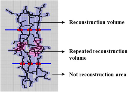
FIGURE 3. Fracture repeated reconstruction area.
In the case of known fracture morphology and fracture permeability, the seepage radius of the fracture facing the reservoir can be obtained, which is expressed as
where r represents the flow radius, m; k represents the permeability of the fracture, mD; t represents time, s; and μ represents the viscosity of the fluid, MPa.
Through the seepage radius of the fracture, the volume of the fracture can be calculated, and the volume coefficient of the repeated reconstruction between the fractures is expressed as
where R represents the volume coefficient of repeated reconstruction; N represents the number of fracture sections;Vc represents the repeated reconstruction volume, m3; and Vi represents the reconstruction volume of the fracture section, m3.
2.2.2 Fracture channeling identification simulation process
The calculation process of the identification method of fracture channeling is shown in Figure 4. The specific calculation steps are as follows: a) According to the actual reservoir size, the connection nodes are divided, and the connection nodes are used for subsequent calculation. b) Combined with geological data, the value of the connection node can be obtained by the interpolation of the existing geological model, including physical parameters and mechanical parameters. c) According to the actual fracturing scale, the perforation data and initial fracture parameters are set. d) The bottom-hole flow pressure at the next time step is calculated according to the construction pump pressure parameters (Eq. 6 and Eq. 7). e) Comparing the bottom-hole flow pressure values of forward calculation and reverse calculation, if not equal, new fracture connection nodes are added (Eq. 8–Eq. 11). f) Steps d ∼ e are repeated until the fitting error is less than the specified error value, and the fracture morphology is output. g) The fracture seepage radius is calculated. h) The repeated reconstruction volume of the parent well is calculated. i) The volume coefficient of repeated reconstruction (fracture channeling coefficient) is calculated, and the quantitative identification of inter-well fracture channeling position is finally realized.

FIGURE 4. Inter-well fracture channeling identification calculation process.
3 Identification and application of fracture channeling in shale reservoirs
3.1 Conceptual model of fracture channeling identification
Based on the identification method of inter-well fracture channeling, a two-well opposite staggered perforation fracturing model is established to quantitatively analyze the location of fracture channeling. The model sets the distance between two wells to be 200 m, and nine clusters of perforations are performed. The cluster spacing is 10 m. The relevant calculated parameters are shown in Table 1.
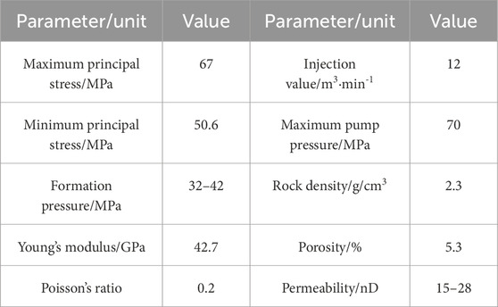
TABLE 1. Basic parameters of the model.
Figure 5 shows the fracture morphology of the two wells after fracturing. The simulation results show that the fracture length of the X1 well is approximately 290 m, and the reconstruction area is 47962 m2. The fracture length of the X2 well is approximately 300 m, and the reconstruction area is 52686 m2. The repeated reconstruction area of the two wells is 8469 m2, and the fracture channeling coefficient of the child well is 16.1%. Figure 6 shows that the fracture channeling area of the two wells occupies nearly half of the seepage intersection area between the two wells, and there is a great risk of fracture channeling.
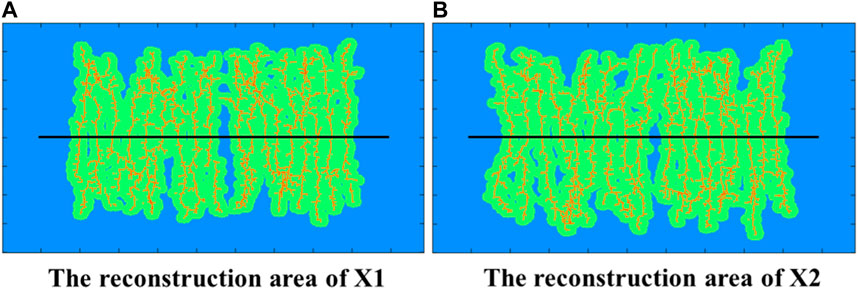
FIGURE 5. Fracture morphology and reconstruction area.
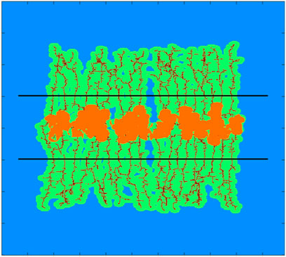
FIGURE 6. Fracturing channeling area between two wells.
3.2 Fracture morphology simulation and channeling analysis in actual blocks
The fractured channeling well in the Weiyuan area is selected as the research object. The reservoir porosity, permeability, and formation pressure coefficient of this well group are low, and the energy supply is insufficient. After fracturing, the reservoir’s physical properties have been improved, but the inter-well fracture channeling is more serious, resulting in great economic losses. According to the existing production dynamic data, the source of fracture channeling in this typical well group has been qualitatively analyzed. At present, it is preliminarily determined that W1, W2, and W3 wells are affected by W4 well fracture channeling, and the specific location is not clear.
According to the method in this paper, the fracturing model of the typical well group is constructed. The actual geological model parameters are the same as those in Table 1, and the simulated fracture morphology is shown in Figures 7B–F.
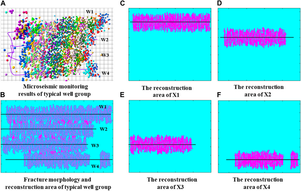
FIGURE 7. Fracture morphology and channeling identification of typical well groups.
The fracture morphology of W1 ∼ W4 wells is shown in Figures 7C–F; Figure 7B shows the reconstruction area after fracturing of the whole well group. A total of 108 sections and 347 clusters of fractures are inverted in the model. The fracture length is between 353 m and 380 m, and the average fracture length exceeds the well spacing (360 m). The simulated fracture length is 87% of the fracture length interpreted by microseismic monitoring. The simulation results are in good agreement with the microseismic monitoring results (Figure 7A).
From the simulation results shown in Figure 7B, there is a certain fracture channeling between wells. In order to further quantify the fracture channeling position, Figure 8 shows the channeling coefficient between each well section. When the channeling coefficient is 8%, it is used as the critical fracturing channeling index, which can be given according to the actual situation. The location of fracture channeling between W1 and W2 wells is mainly distributed in the 8–9, 15, and 29–31 sections. The fracture channeling positions between W2 and W3 wells are mainly distributed in 13, 17, and 25 sections. The location of fracture channeling between wells W3 and W4 is mainly distributed in 11 and 18 sections. It can be analyzed that the W4 well is channeled to the W3 well through 11 and 18 sections and the W3 well is channeled to W2 through 13 and 17 sections and then channeled to W1 through 8 and 15 sections of W2, thus affecting the whole well group, which is consistent with the actual results.
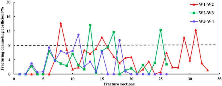
FIGURE 8. Distribution of fracture channeling coefficient in each well section.
It is worth noting that in this paper, the actual fracturing data fitting method is used to constrain the fracture morphology, which depends on the accuracy of the pressure calculation in the fracture. However, the calculation of fracture pressure and fracture filtration used in this paper does not take into account the fluid–solid coupling effect of the reservoir. Therefore, in the follow-up study, the influence of fluid–solid coupling on fracture morphology needs to be further considered.
4 Conclusion
In this paper, a fracture inversion model based on the connection element method is established, which takes into account the fitting of actual fracturing parameters and fracture parameters. In addition, the pressure channeling index is established to quantitatively describe the location of fracture channeling. At the same time, conceptual cases and actual cases are established to verify the accuracy of the model. The main conclusions are as follows:
(1) In the model, the bottom-hole flowing pressure (pwp) calculated by considering the construction pump pressure and the wellbore flow is used to constrain the bottom-hole flowing pressure (pwf) calculated by the construction displacement and fracture morphology, so as to realize the dynamic fitting of the fracture morphology.
(2) Based on the fracture inversion model, the seepage radius of the fracture is considered, and the volume coefficient of repeated reconstruction is used as the quantitative evaluation index of fracture channeling, so as to establish the quantitative identification model of fracture channeling. Through the calculation of the conceptual model, the model can accurately identify the location of channeling.
(3) The actual fracture channeling well group was used for the quantitative analysis of fracture channeling. A total of 108 fractures were simulated. The fracture channeling well section was quantitatively identified by combining the fracture repeated reconstruction volume, and the reason of cross-well fracture channeling is analyzed. The conclusion is consistent with the actual result.
Data availability statement
The original contributions presented in the study are included in the article/Supplementary Material; further inquiries can be directed to the corresponding author.
Author contributions
FH: data curation, methodology, writing–original draft, and writing–review and editing. MY: data curation, methodology, writing–original draft, and writing–review and editing. YZ: data curation, methodology, writing–original draft, and writing–review and editing. HH: data curation and writing–review and editing. WJ: software and writing–review and editing. LL: software and writing–review and editing. CQ: methodology and writing–review and editing. PS: validation and writing–review and editing.
Funding
The authors declare that no financial support was received for the research, authorship, and/or publication of this article.
Conflict of interest
Authors FH, MY, YZ, HH, WJ, LL, CQ, and PS were employed by CNPC Chuanqing Drilling Engineering Co., Ltd.
Publisher’s note
All claims expressed in this article are solely those of the authors and do not necessarily represent those of their affiliated organizations, or those of the publisher, the editors, and the reviewers. Any product that may be evaluated in this article, or claim that may be made by its manufacturer, is not guaranteed or endorsed by the publisher.
References
Ajani, A., and Kelkar, M. “Interference study in shale plays,” in Proceedings of the SPE Hydraulic Fracturing Technology Conference and Exhibition, Woodlands, TX, USA, February 2012.
Aleksandrov, V., Kadyrov, m, Ponomarev, A., Drugov, D., and Bulgakova, I. (2018). Microseismic multistage formation hydraulic fracturing (MFHF) monitoring analysis results. Key Eng. Mater. 785, 107–117. doi:10.4028/www.scientific.net/kem.785.107
Brigham, W., and Smith, D. “Prediction of tracer behavior in fivespot flow,” in Proceedings of the Conference on Production Research and Engineering, Tulsa, Oklahoma, May 1965.
Dali Taleghani, A. (2010). Fracture re-initiation as a possible branching mechanism during hydraulic fracturing. Salt Lake City, Utah: Omnipress.
Du, J., Liu, H., Ma, D., Fu, J., Wang, Y., and Zhou, T. (2014). Discussion on effective development techniques for continental tight oil in China. Petroleum Explor. Dev. 41 (2), 217–224. doi:10.1016/s1876-3804(14)60025-2
Escobar, F. H., Prada, E. F., and Suescún-Díaz, D. (2021). Interpretation of pressure interference tests for wells connected by a large hydraulic fracture. J. Petroleum Explor. Prod. Technol. 11 (8), 3255–3265. doi:10.1007/s13202-021-01249-4
Feng, Y., and Kang, H. (2013). The initiation of Ⅰ-Ⅱ mixed mode crack subjected to hydraulic pressure in brittle rock under compression. J. China Coal Soc. (2), 226–232. doi:10.13225/j.cnki.jccs.2013.02.003
Fu, Y., (2020). How far can hydraulic fractures go? A comparative analysis of water flowback, tracer, and microseismic data from the Horn River Basin. Mar. Petroleum Geol. 115, 104259. doi:10.1016/j.marpetgeo.2020.104259
Geng, Y., Song, Z., Yan, Y., Chen, D., and Wang, L. (2017). Research and application of productivity monitoring technology using new tracer. J. Yangtze Univ. Nat. Sci. Ed. 14 (23), 83–86+7. doi:10.16772/j.cnki.1673-1409.2017.23.017
He, L., Yuan, S., and Gong, W. (2020). Influencing factors and preventing measures of intra-well frac hit in shale gas. Petroleum Reserv. Eval. Dev. 10 (05), 63–69. doi:10.13809/j.cnki.cn32-1825/te.2020.05.009
Huang, L., Lu, M., Sheng, G., Gong, J., and Ruan, J. (2021b). Research advance on prediction and optimization for fracture propagation in stimulated unconventional reservoirs. Lithosphere 2021. doi:10.2113/2022/4442001
Huang, L., Sheng, G., Chen, Y., Zhao, H., Luo, B., and Ren, T. (2022). A new calculation approach of heterogeneous fractal dimensions in complex hydraulic fractures and its application. J. Petroleum Sci. Eng. 219, 111106. doi:10.1016/j.petrol.2022.111106
Huang, L., Sheng, G., Li, S., Tong, G., Wang, S., Peng, X., et al. (2021a). A review of flow mechanism and inversion methods of fracture network in shale gas reservoirs. Geofluids 2021, 1–10. doi:10.1155/2021/6689698
King, G. E., Rainbolt, M. F., and Swanson, C. “Frac hit induced production losses: evaluating root causes, damage location, possible prevention methods and success of remedial treatments,” in Proceedings of the SPE Annual Technical Conference and Exhibition?, San Antonio, TX, USA, October 2017.
Kresse, O., and Weng, X. (2018). Numerical modeling of 3D hydraulic fractures interaction in complex naturally fractured formations. Rock Mech. Rock Eng. 51 (12), 3863–3881. doi:10.1007/s00603-018-1539-5
Li, L., and Wang, T. (2005). Extended finite element method (XFEM) and its application. Adv. Mech. (1), 5–20. doi:10.3321/j.issn:1000-0992.2005.01.002
Meng, L., Bao, W., Guo, B., Shen, J. W., and Sun, H. (2022). Research progress of tracer technology in fracturing effect evaluation. Petrochem. Ind. Appl. 41 (3), 1–4. doi:10.3969/j.issn.1673-5285.2022.03.001
Olson, J. E. “Multi-fracture propagation modeling: applications to hydraulic fracturing in shales and tight gas sands,” in Proceedings of the the 42nd U.S. Rock Mechanics Symposium (USRMS), San Francisco, CA, USA, June 2008.
Puneet, S., Ripudaman, M., Ashish, K., and Sharma, M. M. (2021). Analyzing pressure interference between horizontal wells during fracturing. J. Petroleum Sci. Eng. 204, 108696. doi:10.1016/j.petrol.2021.108696
Sheng, G., Zhao, H., Ma, J., Huang, H., Deng, H. Y., Zhan, W. T., et al. (2023). A new approach for flow simulation in complex hydraulic fracture morphology and its application: fracture connection element method. Petroleum Sci. 20, 3002–3012. doi:10.1016/j.petsci.2023.03.026
Wang, Y., Lu, Y., Li, Y., Wang, X., Yan, X., and Zhang, Z. (2012). Progress and application of hydraulic fracturing technology in unconventional reservoir. Acta Pet. Sin. 33 (S1), 149.
Weng, X., Kresse, O., Cohen, C., Wu, R., and Gu, H. (2011). Modeling of hydraulic-fracture-network propagation in a naturally fractured formation. SPE Prod. Operations 26 (4), 368–380. doi:10.2118/140253-pa
Wu, F., Yan, Y., and Yi, C. (2017). Real-time microseismic monitoring technology for hydraulic fracturing in shale gas reservoirs: a case study from the Southern Sichuan Basin. Nat. Gas. Ind. B 4 (1), 68–71. doi:10.1016/j.ngib.2017.07.010
Zhang, B., Tian, X., Ji, B., Zhao, J., Zhu, Z., and Yin, S. (2019). Study on microseismic mechanism of hydro-fracture propagation in shale. J. Petroleum Sci. Eng. 178, 711–722. doi:10.1016/j.petrol.2019.03.085
Zhao, B., Panthi, K., and Mohanty, K. K. (2020a). Tracer eluting proppants for hydraulic fracture characterization. J. Petroleum Sci. Eng. 190, 107048. doi:10.1016/j.petrol.2020.107048
Zhao, H., Sheng, G., Huang, L., Ma, J., Ye, Y., and Leng, R. (2020b). Calculation of reservoir fracture network propagation based on lightning breakdown path simulation. Sci-entia Sin. Technol. 52, 499–510. doi:10.1360/sst-2020-0406
Zhao, H., Sheng, G., Huang, L., Zhong, X., Fu, J., Zhou, Y., et al. (2021). “Application of lightning breakdown simulation in inversion of induced fracture network morphology in stimulated reservoirs,” in Proceedings of the International Petroleum Technology Conference, San Francisco, CA, USA, March 2021. doi:10.2523/IPTC21157-MS
Keywords: shale reservoir, fracture propagation, data-driven, dynamic fitting, fracture channeling identification, numerical simulation
Citation: He F, Yue M, Zhou Y, He H, Jiang W, Liu L, Qian C and Shu P (2024) Research on the data-driven inter-well fracture channeling identification method for shale gas reservoirs. Front. Earth Sci. 12:1371219. doi: 10.3389/feart.2024.1371219
Received: 16 January 2024; Accepted: 06 February 2024;
Published: 23 February 2024.
Edited by:
Xixin Wang, Yangtze University, ChinaReviewed by:
Yadong Chen, Southwest Petroleum University, ChinaYunfeng Xu, Yangtze University, China
Copyright © 2024 He, Yue, Zhou, He, Jiang, Liu, Qian and Shu. This is an open-access article distributed under the terms of the Creative Commons Attribution License (CC BY). The use, distribution or reproduction in other forums is permitted, provided the original author(s) and the copyright owner(s) are credited and that the original publication in this journal is cited, in accordance with accepted academic practice. No use, distribution or reproduction is permitted which does not comply with these terms.
*Correspondence: Feng He, 1264485659@qq.com