Improved Gaussian regression model for retrieving ground methane levels by considering vertical profile features

1 Introduction

Methane is a major greenhouse gas and studies have shown it to be the second largest contributor to the enhanced greenhouse effect in the atmosphere (Skeie et al., 2023). Atmospheric methane levels have been rising steadily since 2007. Up to now, current atmospheric methane levels have reached approximately 2.5 times pre-industrial levels (Basu et al., 2022). Between 2008 and 2017, researchers estimated that approximately 60% of total global methane emissions were directly attributable to human activities (Saunois et al., 2020). Unlike the long-lived gas carbon dioxide, methane is a short-lived gas whose accumulation in the atmosphere can be reduced in a relatively short time (Rotmans et al., 1990). This means short-term changes in methane are directly reflected in climate change, allowing anthropogenic interventions to significantly impact global warming over a short timeframe. Therefore, monitoring changes in atmospheric methane concentration levels is crucial, but there are presently some shortcomings in the monitoring of methane concentration changes (Wang et al., 2021; Pei et al., 2023; Tianqi et al., 2023).

The European Copernicus Atmospheric Monitoring Service (CAMS) uses atmospheric retrieving modeling incorporating physical and chemical mechanisms to produce reanalyzed data on the global spatial and temporal distribution of methane (Agustí-Panareda et al., 2023). This is based on a priori inputs, including emission inventories and surface station observations. However, the resolution of the CAMS reanalyzed data is relatively coarse. Moreover, the accuracy of the reanalyzed data depends heavily on the a priori inputs from the sparse surface monitoring network (Stein et al., 2014). The current ground-based monitoring network is mainly the Global Atmosphere Watch (GAW) program, coordinated by the World Meteorological Organization (WMO) through collaboration with approximately 100 participating countries globally. The observational data is archived in the World Data Centre for Greenhouse Gases. The heterogeneous geographic distribution of the ground-based data results in significant uncertainty in the reanalyzed data for regions with sparse distribution of monitoring stations (Pei et al., 2022; Liu et al., 2023; Zhang et al., 2023).

Remote sensing techniques provide a large amount of large-scale methane concentration data in contrast to traditional ground-based monitoring methods, including the use of satellites such as TROPOMI and GOSAT (de Gouw et al., 2020; Sadavarte et al., 2021; Suto et al., 2021; Wu et al., 2022). However, it is important to note that the methane concentrations obtained by satellites mainly consist of molar fractions of methane in the atmospheric column-averaged dry air (Schneising et al., 2019), which may not precisely reflect ground-level methane levels (Shi et al., 2021; Shi et al., 2023). Considering the high concentration of human production and living space on the ground, it is necessary to acquire ground methane concentration data for monitoring sources and changes in methane (Yang et al., 2023).

Due to the constraints and specific qualities of the mentioned data sources, one could potentially infer the level of methane concentration at the ground by consolidating numerous sources of information, such as the vertical distribution of methane in the atmospheric chemistry model data and satellite observation data. Relevant researchers obtained methane concentrations at the ground by fitting the atmospheric chemistry model simulation data with a Gaussian function to compute the methane concentration data at the ground level (Xu et al., 2021). However, due to the highly inadequate resolution of the atmospheric chemistry model data, the outcome achieved is also a general statistical result. Based on this method, researchers compared the simulated ground-level methane concentration data using a Gaussian function based on an atmospheric chemistry model with total methane column concentrations (Qin et al., 2023). After determining the proportion of ground-level methane concentration in the total methane column concentration, researchers can use this to convert the methane column concentration data collected by the satellite to ground-level methane concentrations. As a result, the ground methane concentrations can be obtained with greater accuracy. However, the results were influenced by the satellite and atmospheric model products, resulting in monthly average CH₄ levels that were gridded to a coarse resolution of 0.1°× 0.1°.

In this study, we proposed an improved method for retrieving ground methane concentrations. It combines the strengths and limitations of each dataset by considering the shortcomings of previous studies. First, we obtained the high-coverage methane column concentrations derived from satellite observations by filling the missing pixels caused by invalid retrievals or cloud masks. This expands our temporal and spatial coverage. Then, the scale factor data were retrieved by fitting altitude and concentration data from atmospheric chemistry model simulations by linear interpolation instead of the Gaussian function. The result of this method can be used for the calculation of the ratio of the ground-level methane concentration to the methane concentration of the column. The ground-level methane concentrations and the methane columns observed by satellites can be used to calculate the ratio. Finally, the results are further corrected using ground station observations according to the Gaussian regression model to obtain highly accurate ground-level methane concentration data.

2 Materials and methods

2.1 Materials

As shown in Figure 1, the study area covers the geographical region of China, extending from 70°E to 140°E and 10°N to 55°N. The data used in our study include the atmospheric methane stratification data of CAMS global greenhouse gas reanalysis (EGG4), the CH₄ product data of TROPOMI as the real observed atmospheric methane column average concentration data, the ground methane concentration data collected by the Global Atmosphere Watch (GAW) network in the world data center for greenhouse gases, which is provided by the Copernicus atmospheric monitoring service, the atmospheric reanalysis data of ERA5 and the ground elevation data of Shuttle Radar Topography Mission (SRTM).

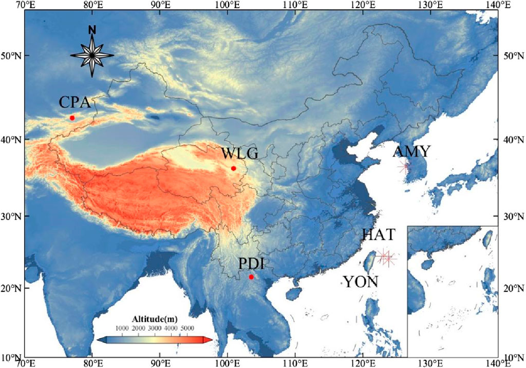
FIGURE 1. Research area considered in this study. It mainly includes the region where the Chinese Mainland is located. Marked are the locations of the ground stations used for validation. The ground-based measurements (WDCGG) from CPA, WLG, PDI, AMY, HAT, and YON are used as validation data.

According to the relevant studies, the EGG4 data from CAMS can display the global trend and seasonal cycle of greenhouse gas concentrations (Inness et al., 2019; Custódio et al., 2022; Agustí-Panareda et al., 2023). This is achieved by combining the model with measurements from different locations using physical and chemical mechanisms, which produces data on the concentration of greenhouse gases globally at different heights from the ground to the top of the atmosphere (Custódio et al., 2022). In this way, methane concentrations at different levels from EGG4 can be used to evaluate changes in the vertical distribution of methane in the atmosphere at different spatial and temporal scales. The EGG4 dataset is divided into 60 model levels, which correspond to 60 altitude layers ranging from the Earth’s ground to the top of the atmosphere (Agusti-Panareda et al., 2017). Our study collected EGG4 data between 1 January 2019, and 31 December 2021. The dataset includes methane column-average molar concentration and vertical profile features, with the former measured in part per billion volume (ppbv) and the latter in kilograms per kilogram (kg·kg-1). Further conversion and processing of this data is required.

Our study used ground methane concentrations from the World Data Centre for Greenhouse Gases (WDCGG) monitoring station located in the study area. The station offers observation from several modes, including surface, tower, aircraft, and ship. This research focused on the primary modes of data collection: surface and tower. Because of the different geographical locations and observation modes of the stations, the heights of the observations vary from one station to another. To validate the data, it is necessary to calculate the observed values of methane concentration at the height of the observation station. The number of WDCGG stations in the 70° to 140°E and 0° to 55°N region is limited, with only six stations: CPA, WLG, PDI, AMY, HAT, and YON. However, the data acquired by EGG4 correspond to only three stations: CPA, WLG, and PDI.

To accurately calculate ground methane concentrations, it is necessary to collect ground elevation to estimate the ground methane concentration. The provided methane concentration data from the atmospheric model has a limited resolution of 0.75°×0.75° and is obtained from simulations, which may differ from actual measurements. Therefore, we use the entire average concentration of methane columns, obtained by inverting the data for XCH₄ from TROPOMI, as actual measurements to correct the result of the atmospheric model.

Details of the dataset used in this study are summarized in Table 1, and all data were resampled to a uniform spatial resolution of 0.05° × 0.05° (equal to approximately 5 km) and averaged daily.

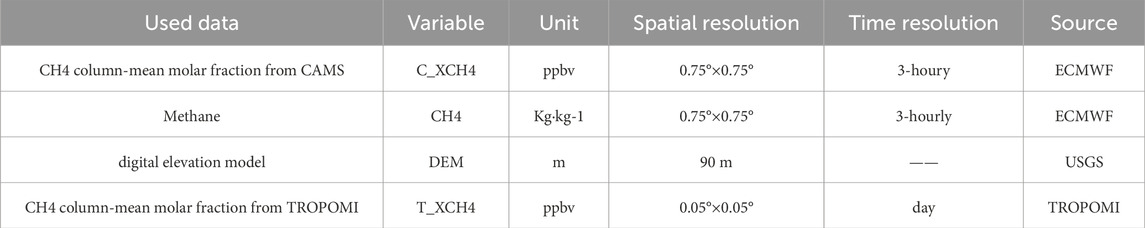
TABLE 1. Dataset used in this study (2019–2021).

2.2 Methods

2.2.1 Methane profile fitting

Firstly, the atmospheric methane profile data was fitted to obtain the methane profile function. This is mainly based on the atmospheric methane layer concentration data provided in CAMS/EGG4 data. The EGG4 atmospheric methane layer data comprises the layer height and the concentration data, which were divided into a total of 60 model levels ranging from the ground to the atmospheric top. The pressure levels corresponding to different model levels are 1000, 950, 925, 900, 850, 800, 700, 600, 500, 400, 300, 250, 200, 150, 100, 70, 50, 30, 20, 10, 7, 5, 3, 2, 1 hPa (Agusti-Panareda et al., 2017). For each location, we obtain the level height and level concentration data and fit them into a function to obtain the atmospheric methane profile function. The specific functions to be used are discussed in the following paragraphs. Here, the symbol “f” is used as an example of the function, and the fitting results are as follows:

Where the fitted atmospheric methane profile function is denoted by C(h), and the methane concentration C at the corresponding height can be obtained by inputting the height h. The function f(h,c) has the height h and the level concentration data c as variables.

It should be noted that the methane stratification data at each spatial and temporal location was fitted by f(h,c) to obtain the methane profile function corresponding to the spatial and temporal locations. The study aims to estimate the ratio between the ground-level methane concentration and the column methane concentration. Therefore, the atmospheric methane concentration and altitude data must be accurately fitted by a methane profile function to obtain an accurate relationship between the methane concentration at a given altitude and the methane concentration in the atmospheric column. Gaussian functions have been used in previous studies to fit the atmospheric methane profile (Qin et al., 2023). As in formula (2-5), in this study, we compared the fitting of Gaussian functions, multinomial Gaussian functions, smooth curve fitting, and linear interpolation fitting, as shown in Figure 2. The following is an introduction to the four fitting methods, and the Gaussian function has the formula,

where f(h) indicates that the independent variable of the fit is a function of height h, that is the methane concentration at height h, and a, b, and c are the parameters of the Gaussian function.

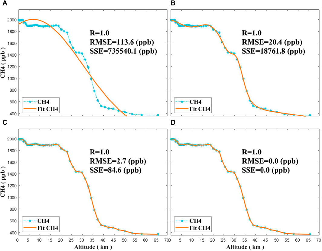
FIGURE 2. Effectiveness of vertical profile features of atmospheric methane via various methods: (A) Gaussian Fit, (B) Multiple Gaussian Fit, (C) Smoothing Spline Fit, and (D) Liner Interp Fit. The blue color in the figure represents the real data, while the orange color represents the fitting results, and the R, RMSE, and SSE of the fitting results using different methods are labeled.

The multiple Gaussian functions fit shall be of the following formula, with two to six Gaussian functions fitted separately to each raster image element, the number of fits taken from related studies (Qin et al., 2023),

where f(h) is the methane concentration at height h and a, b, and c are parameters of a Gaussian function where n = 2, 3, 4, 5, 6. By setting n=2 to 6 respectively, the fitting error can be calculated, and the n-value corresponding to the minimum fitting error can be found, which will be used as the n-value for fitting multiple Gaussian functions at that position. Smooth linear fitting constructs a coefficient by weighting the sum of the squared residuals and the sum of the rates of change of the curves of one of the fitted functions. This is used to find the best-fitting function.

Where f(h) is the methane concentration at height h. The $w_i$ is the weight, which is 1 if it is not present. Here the weight refers to the importance of the different altitudes and the corresponding methane concentration data. As the importance of all the data is the same, the weight is ‘not present’. Therefore, the weight is 1. The variable p is a value in the range [0,1] and is called the smoothing parameter (smoothing coefficient), and the smaller the value of p, the smoother the fitting result. Because the height h and the methane concentration c of different layers obtained in the study are unweighted, $w_i$ is always 1. The purpose of this fitting is to obtain the atmospheric methane profile function, so no smoothing was applied, and then p was set to 1. This allows the fitted function curve to pass through as many points as possible, which are composed of fitted elevation and methane concentration data.

Considering that non-smoothing of the data better meets the requirements of the study, while linear interpolation does not perform any operations on the data, the study considers using the linear interpolation method for testing. The formula for linear interpolation is as follows.

where f(H) is the methane concentration at height h.

The 60 model levels of EGG4 data were used to fit the atmospheric methane profile function and the results are shown in Figure 2. Compared with direct Gaussian regression, multiple Gaussian regression and smooth linear fitting can fit the results better, but there is still an error between the results and the sample data. The R (Correlation Coefficient) between the linear interpolation results and the real values is 1 and the RMSE (Root Mean Square Error) and the MAE (Mean Absolute Error) are both 0. Compared with the other three methods, linear interpolation can provide the best results and thus estimate the surface methane concentration more accurately. Therefore, linear interpolation fitting was used to obtain information on the vertical distribution of atmospheric methane.

2.2.2 Extracting methane profile features

After fitting the atmospheric methane profile function by linear interpolation fitting, the methane concentration can be calculated by substituting the data at any height into the function. Then, as shown in Eq. 6, it is possible to obtain the ratio of the methane concentration at any height to the total atmospheric methane column concentration, or the ratio of the methane column concentration to the total atmospheric methane column concentration in any range of heights.

where Ratio is the calculated scaling factor, C(h) is the methane concentration at height h, and Col is the methane column concentration corresponding to the model data.

It is important to note that the methane profile function and concentration data here are both methane data simulated by the atmospheric model. Here, the atmospheric methane profile function at each image position is calculated separately for that position, and the profile function and scale information are also only applicable to that position and time point to improve the accuracy of the estimation.

2.2.3 Estimating ground methane concentrations

Using the above method, we have obtained the characteristics of the vertical distribution of the atmospheric methane from the atmospheric model data. The above methods can be used to obtain preliminary surface methane concentrations. However, the data used in the above methods are inherently uncertain, especially in areas with fewer ground stations (Stein et al., 2014; Danilo et al., 2022). Therefore, the uncertainty of the surface methane concentration obtained by the above method is relatively high. However, satellite observation data, which has broader coverage and is not influenced by the distribution of ground stations, is recommended for obtaining more accurate results. Satellite data provides more accurate observations of the situation (Inness et al., 2022). Therefore, it is recommendable to use satellite methane data instead of methane data simulated by an atmospheric model as real data. Additionally, the scale information obtained from the atmospheric model data is used to transform the CH₄ column-mean molar fraction data into ground-level methane concentration data, which needs standardization of unit measurements. The satellite-based methane data displays the average methane concentration throughout the entire atmospheric column.

To enhance accuracy and reduce computational steps, the methane ratio calculation has been adjusted to the ratio of methane concentration at any height to the average concentration of the entire methane column. This result is unchanged. Thus, the ground-level methane concentration is calculated.

where SurfaceCH₄ is the ground methane concentrations, T_Col is defined as the total column concentration of methane observed by satellites, which is the cumulative value of methane concentration in the column from the surface to the atmosphere. However, the result of the satellite observation data is the average concentration of the methane columns, which means that it is the average value of T_Col, also known as the mean(T_Col). C(h) is the methane concentration at height h, and Col is the methane column concentration corresponding to the EGG4 data. Therefore, when calculating the column concentration based on EGG4 data, it is necessary to calculate the column average concentration mean(Col) to facilitate unit unity with satellite data. The atmospheric model data were calibrated using CH₄ column-average molar fraction data observed by satellite through the method described above.

2.2.4 Correcting ground methane concentrations

Significant deviations were observed between the ground methane concentration data collected through this method and the actual data. Our research uses Gaussian Process Regression (GPR) (Rasmussen et al., 2003) models to construct machine-learning regression models to address this bias. Gaussian process regression is the use of Gaussian processes for the solution of regression problems.

Where f(x) follows a Gaussian distribution $GP\left(0,\mathrm{k}\left(x,x^{\prime }\right)\right)$. $\mathrm{k}\left(x,x^{\prime }\right)$ denotes the basis function, which is the covariance between the features of each variable that can be modeled by a Gaussian process kernel. h(x) denotes the transformation function that transforms the sample feature x into the target feature h(x). Therefore, the response function of the Gaussian process regression can be described as,

Where y_i is the target characteristics under x_i, ${\sigma }^2$ is the error variance, β is the coefficients, all estimated from sample data.

GPR models are nonparametric, kernel-based, and probabilistic. As a result, they do not need specific model forms and can deal with nonlinear associations. Additionally, the covariance matrix is used by the Gaussian process regression to represent the correlation between the sample data. This enables a seamless transition and generalization of the model, making it very helpful for dealing with data with correlation. The method provides excellent generalization ability even with small sample sizes. This study constructed a Gaussian process regression model using the station’s observed ground methane concentration as the dependent variable and the pre-estimated ground methane concentration, topographic data, time variables, and location information as the independent variables. Using this method, ground-level methane concentration data can be computed with a high degree of precision.

2.2.5 Accuracy verification

To ensure the accuracy of the modeling of ground-level methane concentrations, real methane data observed at ground stations were used for validation. Due to the varying heights of the stations, it was necessary to estimate methane concentrations at the station heights for comparison with the station data during validation.

In addition, to ensure the accuracy of the calibration of the Gaussian regression model, the accuracy of the model can be evaluated using ten-fold cross-validation. Cross-validation can reduce the possibility of evaluation results being affected by data partitioning methods and verify the generalization performance of the model, compared to simply dividing the training and testing sets. Due to limitations in the number of ground stations and research time frame, the sample data used in the experiment is limited. Additionally, cross-validation can more fully utilize the limited data since the amount of the final sample data used for training the model is only 1710. It is common to choose a 5 or 10 fold cross validation when using this method. Due to smaller datasets, 10-fold cross-validation may be more suitable as it provides more training data and more frequent model evaluations. The data are randomly divided into ten parts, with one segment reserved as the test set and the remaining nine used as the training set. After repeating this process ten times, the accuracy of the simulated CH₄ column concentrations is evaluated using R², RMSE, and MAE calculations (He et al., 2021).

These formulas are calculated as follows:

where x, y represent the CH4 measurements and the model-fitted CH₄ levels, respectively.

where X_i is the model fitted CH₄ result, $\overline{\mathrm{X}}$ is the mean of the model fitted result and n is the total number of data bars.

where $Y_i$ is the model fitted CH₄ result, $\overline{\mathrm{Y}}$ is the mean of the model fitted result and n is the total number of data bars.

3 Results

3.1 Accuracy verification of the proposed method

As shown in Figure 3, comparing the ground-level methane concentration corrected by satellite observation data with the station observation methane concentration data, it can be found that there is still a general bias, and the correlation coefficient between the estimated methane concentration at the height of the station and the real methane concentration is 0.66, with an average bias of 44 ppbv. The estimated surface methane concentration reflects the trend of methane concentration over time to some extent when compared with actual observation data from ground stations. However, there is an overall deviation between the estimated surface methane concentration and the actual observed data.

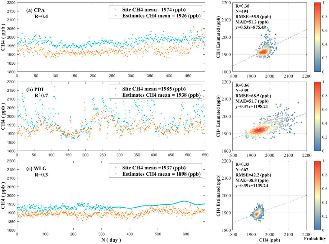
FIGURE 3. Comparison of ground-level methane concentration data after correction of satellite data with station observations of methane concentrations. The figure on the left (A–C) shows the average of the model’s fitting results at station CPA, PDI, and WLG with the real data, as well as the correlation coefficient R (rounded to one decimal place) between the two. The figure on the right presents the number of real data and fitting results at each site location, the correlation coefficient R (rounded to two decimal places), the RMSE, the MAE, and the univariate linear functions fitted from the data.

As shown in Figure 3, there is a bias in the estimated ground methane concentration, so the study used a Gaussian process regression model for correction. To ensure the reliability of the corrected model, it was tested by ten-fold cross-validation. The model’s results were different because of the different settings of the kernel function in the Gaussian regression model. Therefore, we compared the results of the model for different cases of kernel functions. Figure 4 shows some typical fit cases, and all the results can be found in Appendix A. The optimal results are achieved by selecting the rational-quadratic kernel function (Figure 4D), which is a parameterized rational-quadratic kernel function. With this kernel function, the tenfold cross-validation correlation coefficient R of the model is 0.93, with an R² of 0.87. The mean absolute error (MAE) is 9.6 ppbv, and the root mean square error is 16.1 ppbv. These values demonstrate the high generalization capability of the model, indicating its ability to estimate the ground-level methane concentration in the unknown region.

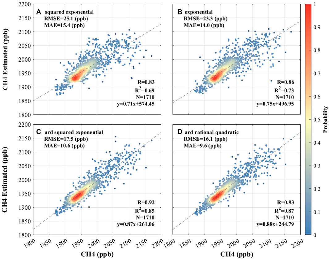
FIGURE 4. Partial Gaussian process regression kernel function selection and results. In panel (A), the squared exponential means Squared exponential kernel. In panel (B), the exponential means Exponential kernel. In panel (C), the ard squared exponential means Squared exponential kernel with a separate length scale per predictor. In panel (D), the ard rational quadratic means Rational quadratic kernel with a separate length scale per predictor.

After applying the Gaussian regression model correction shown in Figure 5, the overall model accuracy improved with an average correlation coefficient R of 0.93. In addition, the mean absolute error (MAE) between the data from the site and the estimated data was 9.6 ppbv. By using the Gaussian regression model to correct the ground-level methane concentration estimated from the satellite data, ground-level methane concentration data can be obtained with a resolution of 0.05° for full coverage of the study area.

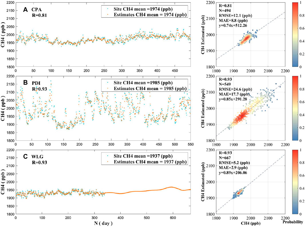
FIGURE 5. Comparison of station-based observations and ground methane concentrations retrieved by the improved Gaussian regression model at stations (A) CPA, (B) PDI, and (C) WLG, using ten-fold cross-validation. The figure on the left (A–C) shows the average of the model’s fitting results at station CPA, PDI, and WLG with the real data, as well as the correlation coefficient R (rounded to two decimal places) between the two. The figure on the right presents the number of real data and fitting results at each site location, the correlation coefficient R (rounded to two decimal places), the RMSE, the MAE, and the univariate linear functions fitted from the data.

3.2 Spatiotemporal characteristics of ground methane concentrations

After collecting data on ground-level methane concentration, we summed the results for each season and year and created a distribution map, as shown in Figure 6. The study found that ground-level methane levels showed an increase to the east and a decrease to the west, as well as a decrease to the north and an increase to the south of China. The study estimates the ground-level methane concentration, which is significantly influenced by both human activities and ecosystems, with local human activities playing a particularly prominent role. Multiple factors contribute to the distribution of ground-level methane. In southeastern China, abundant water resources, a dense population, and frequent agricultural activities result in higher methane emissions from livestock and rice cultivation than in the northwestern region (Peng et al., 2016). Abundant water resources support abundant wetlands, which provide more suitable conditions for anaerobic bacteria to produce methane (Keppler et al., 2006; Bloom et al., 2010). In contrast, the western region has fewer water resources and more arid areas, resulting in more methane from this source in the east and south than in the west. The southeastern region, due to its proximity to the ocean and higher temperature, has more water vapor, which is more conducive to methane production. This condition also encourages the cyclic reaction of methane in the atmosphere, resulting in greater methane production in the coastal areas of the east and south compared to the inland regions (Rotmans et al., 1990; Sass et al., 1991). However, certain special circumstances, such as increased chemical reactions in the atmosphere, can cause atmospheric methane levels to be lower in this region (Methane escapes from major city, 2015). In addition, CH₄ emissions from urbanization and industrialization can increase in economically developed regions. As a result, a distribution pattern is formed, as shown in Figure 6.

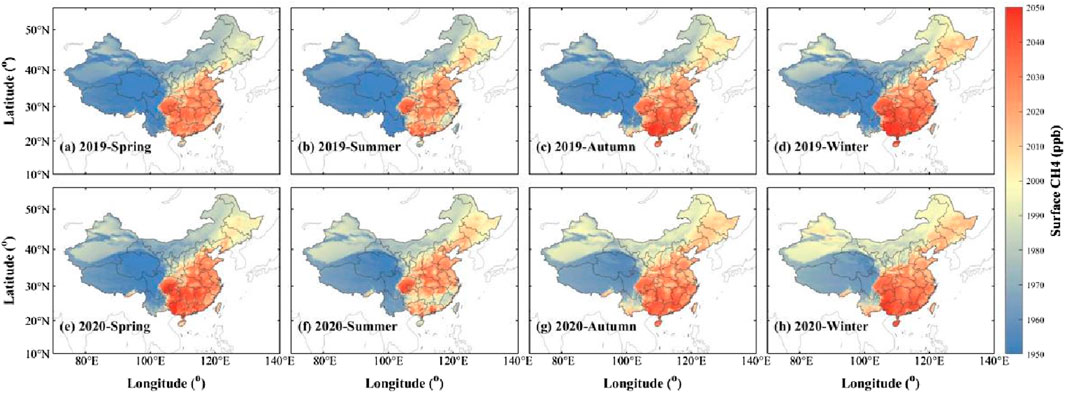
FIGURE 6. Ground-level Methane Concentration distribution in different seasons: (A–D) shows the average results of ground methane concentration for the four seasons in 2019, and (E–H) shows that for 2020. The seasons are divided into March-May for spring, June-August for summer, September-November for autumn, and December-February for winter.

Figure 6 shows ground-level methane concentration distribution in different seasons. The seasons are divided into March-May for spring, June-August for summer, September-November for autumn, and December-February for winter. Ground-level methane concentrations show higher levels during autumn and winter and lower levels in spring and summer. In urban areas, methane concentrations are higher in winter, similar to previous studies (Thomas and Zachariah, 2012; Vinogradova et al., 2022). During autumn and winter, lower temperatures result in reduced atmospheric movement, which leads to increased stability and weak upward diffusion of atmospheric methane (Guo et al., 2023). In addition, vegetation respiration is reduced, and this reduced respiration may reduce the ability of vegetation and soils to absorb atmospheric methane, contributing to increased ground-level methane concentrations (Han et al., 2023). Methane production is more favorable during periods of high humidity and anaerobic conditions in autumn and winter than in spring and summer (Thauer, 2010; Song et al., 2021). Moreover, energy consumption increases during the autumn and winter months, while human energy activities may lead to an increase in methane emissions (Hmiel et al., 2020).

In the southern part of the studied region, the change in methane concentration is relatively small and its concentration is lower. So, as shown in Figure 6, after annual averaging of the data and displaying the results on a larger scale, the southern part of the study area in the figure seems to have the same CH4 concentration. We have therefore narrowed down the range of concentrations displayed and the spatio-temporal range, as shown in Figure 7, which shows the methane concentration in the southern part of the study area on a single day. As shown in the figure, the study can discover fine changes in the daily surface methane concentration, which can be used to monitor changes in methane concentration in small areas.

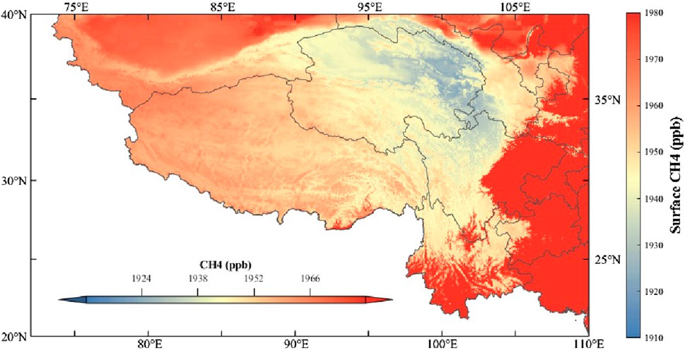
FIGURE 7. Distribution of ground-level methane concentrations in southwest China over 1 day.

3.3 Distribution of the ground methane concentrations in Shandong Province

In this study, we thoroughly explored the ground-level methane concentration in Shandong Province. As shown in Figure 8, we obtained the monthly mean distribution graph of the ground-level methane concentration in Shandong Province. By looking carefully at the graph, we found that the ground-level methane concentration in Shandong Province showed an increasing and then a decreasing trend during the year. It is worth mentioning that, the methane concentration in the inland areas of Shandong Province is significantly higher than that in the coastal areas. From the data, it is clear that the surface methane concentration in Shandong Province shows cyclical changes over time, and that these cyclical changes may be influenced by factors such as temperature and vegetation cover. This result provides important information for a better understanding of the spatial and temporal distribution of methane and also provides insight into the search for the specific sources leading to the large increase in methane. Meanwhile, comparing methane concentrations in inland and coastal areas of Shandong Province, we found a clear difference in the geographical distribution. Such differences may be related to human activities, land use, and other factors in different regions. An accurate study of these differences will help us gain a more detailed insight into the sources and influencing factors of methane emissions. Taking Shandong Province as an example, based on the trends of methane concentration in different regions, the government can take targeted measures to reduce methane emissions and promote the application of low-carbon development policies. This targeted policy formulation will be more precise and help improve the effectiveness of environmental protection and carbon emission reduction, providing a scientific basis for sustainable development.

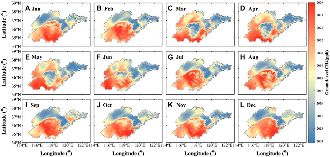
FIGURE 8. Distribution of monthly mean values of ground-level methane concentration in Shandong Province from 2019 to 2020: (A–J) show the distribution of surface methane concentration from January to December. The colors in the picture correspond to the color bar on the right.

4 Discussion

4.1 Comparison with other studies

In comparison to the existing satellite observation data products and ground station observation data products (Alexe et al., 2015), the method in this study can estimate the ground-level methane concentration data in any land area. Additionally, the satellite observation data primarily provide column concentration data products from the ground to the top of the atmosphere, rather than ground-level methane concentration data. The distribution of ground stations is too sparse, and their observations can only describe the methane concentration within a certain range around the stations.

Compared to the atmospheric model data (DalsøRen et al., 2016), the atmospheric model estimated methane concentration data include methane column concentration data in the whole atmosphere as well as layered atmospheric methane concentration data. However, the resolution of the atmospheric model data is extremely low and it is only suitable for studying the variation of methane concentration at ground level on a large scale, such as the world. Our method used in this study has the ability to estimate ground-level methane concentrations with greater accuracy at a resolution of 0.05°× 0.05°. Therefore, it is possible to study changes in the ground-level methane distribution at a more detailed scale. Moreover, the distribution of ground stations has a strong influence on the methane data source for the atmospheric model data.

Compared with other related methods (Qin et al., 2023; DalsøRen et al., 2016), some of their sources of methane concentration data are atmospheric model data, which may have a bias between them and the actual atmospheric methane concentration, and some of them use satellite observation data as their sources of methane concentration data, but the resolution of their acquired data products is lower than 0.1°in the Chinese region, and the time resolution is monthly. Our research method balances the advantages of the above methods. In this study, the temporal and spatial resolution of the estimated ground-level methane data was improved to the daily resolution and 0.05°×0.05°resolution based on the satellite observation data as the real methane concentration data. Our results are highly accurate, with a ten-fold cross-validation R of 0.93, an R² of 0.87, a mean absolute error (MAE) of 9.6 ppbv, and a root mean square error (RMSE) of 16.1 ppbv.

4.2 Methodology critical analysis

The method used in this study has the advantage of obtaining large-scale, high spatiotemporal resolution surface methane concentration data, as demonstrated in the previous text. However, it is important to note that this study has some limitations due to factors such as the data and methods used in the study. Firstly, the atmospheric methane vertical profile function fitted by atmospheric model data was used to calculate ground methane concentration in the previous part of the study. However, atmospheric model data inherently contains uncertainty, and the fitting function may not be able to produce completely realistic results. This can affect the simulated atmospheric methane vertical profile function and the calculation of ground methane concentration, resulting in uncertainty. Furthermore, satellite observation data will be used as real observation data to correct the simulated ground methane concentration mentioned above. However, satellite observation data provides high-coverage reconstructions, which can introduce uncertainty when used for estimation. Finally, the Gaussian regression method cannot perfectly estimate all the data, and R is not equal to one. Therefore, as shown in Figure 5, the estimated ground-level method concentrations may exhibit a high level of agreement with the site data in terms of mean bias, but there may be either a lower or upper bias on a daily basis.

5 Conclusion

At present, it is difficult to obtain large-scale ground-level methane concentration data from satellite and ground station observations. In this paper, a method is provided to estimate the ground-level concentration based on satellite monitoring data and atmospheric model data by using Gaussian regression correction and atmospheric methane profile fitting. Through this method, our study obtained highly accurate ground-level methane concentration data. Compared with WDCGG ground-level monitoring station data, the basis of estimated ground-level methane concentration is less than 10 ppbv, and ten-fold cross-validation has R of 0.93 and R² of 0.87. The current results will be affected by the uncertainty of the atmospheric model data and satellite observation data used, as well as the influence of the Gaussian regression correction model used, resulting in the estimated surface metal concentration being a small bias daily. Of course, the estimated ground-level method concentrations may exhibit a high level of agreement with the site data in terms of mean bias.

Overall, the method used in this paper can estimate the ground-level methane concentration in different regions for a long period. Through experimental analysis, the method can be used to study the distribution and cyclical changes of ground-level methane, which has potential applications in carbon source monitoring, carbon emission measurement, and analysis of spatial and temporal changes of greenhouse gases.

In the future, we will evaluate the performance of the proposed model at different time intervals (including monthly, seasonal, and annual scales) and test methane concentrations at different surface altitudes.

Data availability statement

The original contributions presented in the study are included in the article/Supplementary material, further inquiries can be directed to the corresponding author.

Author contributions

HH: Conceptualization, Methodology, Writing–original draft, Writing–review and editing. TZ: Formal Analysis, Investigation, Writing–original draft, Writing–review and editing. JZ: Investigation, Visualization, Writing–original draft, Writing–review and editing. XY: Software, Validation, Writing–original draft, Writing–review and editing. ES: Investigation, Methodology, Writing–original draft, Writing–review and editing. HL: Formal Analysis, Visualization, Writing–original draft, Writing–review and editing. HZ: Data curation, Software, Writing–original draft, Writing–review and editing. XL: Resources, Validation, Writing–original draft, Writing–review and editing. GL: Resources, Software, Writing–original draft, Writing–review and editing. YZ: Investigation, Validation, Writing–original draft, Writing–review and editing. ZJ: Conceptualization, Methodology, Validation, Visualization, Writing–original draft, Writing–review and editing. WW: Funding acquisition, Supervision, Writing–review and editing.

Funding

The author(s) declare that financial support was received for the research, authorship, and/or publication of this article. This study was supported by the National Natural Science Foundation of China (42371392), Basic Science-Center Project of National Natural Science Foundation of China (72088101), Natural Science Foundation of Hunan Province, China (2023JJ30660), and the Key Program of the National Natural Science Foundation of China (41930108).

Acknowledgments

We express our sincere gratitude to those who provided support and advice for this article.

Conflict of interest

Authors HH, TZ, JZ, XY, ES, HL, HZ, XL, GL, and YZ were employed by Sinopec Shengli Oilfield Technology Testing Center.

The remaining authors declare that the research was conducted in the absence of any commercial or financial relationships that could be construed as a potential conflict of interest.

Publisher’s note

All claims expressed in this article are solely those of the authors and do not necessarily represent those of their affiliated organizations, or those of the publisher, the editors and the reviewers. Any product that may be evaluated in this article, or claim that may be made by its manufacturer, is not guaranteed or endorsed by the publisher.

References

Appendix A

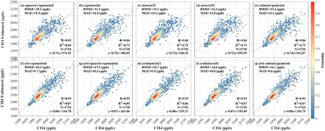
FIGURE A1. Gaussian process regression kernel function selection and results. (A) squared exponential means Squared exponential kernel. (B) exponential means Exponential kernel. (C) matern32 means Matern kernel with parameter 3/2. (D) matern52 means Matern kernel with parameter 5/2. (E) rational quadratic means Rational quadratic kernel. (F) ard exponential means Exponential kernel with a separate length scale per predictor. (G) ard squared exponential means Squared exponential kernel with a separate length scale per predictor. (H) ardmatern32 means Matern kernel with parameter 3/2 and a separate length scale per predictor. (I) ardmatern52 means Matern kernel with parameter 5/2 and a separate length scale per predictor. (J) ard rational quadratic means Rational quadratic kernel with a separate length scale per predictor.

References

Agustí-Panareda, A., Barré, J., Massart, S., Inness, A., Aben, I., Ades, M., et al. (2023). Technical note: the CAMS greenhouse gas reanalysis from 2003 to 2020. Atmos. Chem. Phys. 23 (6), 3829–3859. doi:10.5194/acp-23-3829-2023
Agusti-Panareda, A., Diamantakis, M., Bayona, V., Klappenbach, F., and Butz, A. (2017). Improving the inter-hemispheric gradient of total column atmospheric CO<sub>2</sub> and CH<sub>4</sub> in simulations with the ECMWF semi-Lagrangian atmospheric global model. Geosci. Model Dev. 10 (1), 1–18. doi:10.5194/gmd-10-1-2017
Alexe, M., Bergamaschi, P., Segers, A., Detmers, R., Butz, A., Hasekamp, O., et al. (2015). Inverse modelling of CH<sub>4</sub> emissions for 2010–2011 using different satellite retrieval products from GOSAT and SCIAMACHY. Atmos. Chem. Phys. 15 (1), 113–133. doi:10.5194/acp-15-113-2015
Basu, S., Lan, X., Dlugokencky, E., Michel, S., Schwietzke, S., Miller, J. B., et al. (2022). Estimating emissions of methane consistent with atmospheric measurements of methane and δ13C of methane. Atmos. Chem. Phys. 22 (23), 15351–15377. doi:10.5194/acp-22-15351-2022
Bloom, A. A., Palmer, P. I., Fraser, A., Reay, D. S., and Frankenberg, C. (2010). Large-scale controls of methanogenesis inferred from methane and gravity spaceborne data. Science 327 (5963), 322–325. doi:10.1126/science.1175176
Custódio, D., Borrego, C., and Relvas, H. (2022). Worldwide evaluation of CAMS-EGG4 CO2 data Re-analysis at the surface level. Toxics 10, 331. doi:10.3390/toxics10060331
DalsøRen, S. B., Myhre, C. L., Myhre, G., Gomez-Pelaez, A. J., Søvde, O. A., Isaksen, I. S. A., et al. (2016). Atmospheric methane evolution the last 40 years. Atmos. Chem. Phys. 16 (5), 3099–3126. doi:10.5194/acp-16-3099-2016
Danilo, C., Carlos, B., and Hélder, R. (2022). Worldwide evaluation of CAMS-EGG4 CO2 data Re-analysis at the surface level. Toxics 10 (6), 331. doi:10.3390/toxics10060331
de Gouw, J. A., Veefkind, J. P., Roosenbrand, E., Dix, B., Lin, J. C., Landgraf, J., et al. (2020). Daily satellite observations of methane from oil and gas production regions in the United States. Sci. Rep. 10 (1), 1379. doi:10.1038/s41598-020-57678-4
Guo, J., Feng, H., Peng, C., Chen, H., Xu, X., Ma, X., et al. (2023). Global climate change increases terrestrial soil CH4 emissions. Glob. Biogeochem. Cycles 37 (1), e2021GB007255. doi:10.1029/2021gb007255
Han, X., Yao, N. N., Wang, X. J., Deng, H. H., Liao, H. X., Fan, S. Q., et al. (2023). Short-term effects of asymmetric day and night warming on soil N2O, CO2 and CH4 emissions: a field experiment with an invasive and native plant. Appl. Soil Ecol. 187, 104831. doi:10.1016/j.apsoil.2023.104831
He, J., Jin, Z., Wang, W., and Zhang, Y. (2021). Mapping seasonal high-resolution PM2.5 concentrations with spatiotemporal bagged-tree model across China. ISPRS Int. J. Geo-Information 10 (10), 676. doi:10.3390/ijgi10100676
Hmiel, B., Petrenko, V. V., Dyonisius, M. N., Buizert, C., Smith, A. M., Place, P. F., et al. (2020). Preindustrial (14)CH(4) indicates greater anthropogenic fossil CH(4) emissions. Nature 578 (7795), 409–412. doi:10.1038/s41586-020-1991-8
Inness, A., Aben, I., Ades, M., Borsdorff, T., Flemming, J., Jones, L., et al. (2022). Assimilation of S5P/TROPOMI carbon monoxide data with the global CAMS near-real-time system. Atmos. Chem. Phys. 22 (21), 14355–14376. doi:10.5194/acp-22-14355-2022
Inness, A., Ades, M., Agustí-Panareda, A., Barré, J., Benedictow, A., Blechschmidt, A. M., et al. (2019). The CAMS reanalysis of atmospheric composition. Atmos. Chem. Phys. 19 (6), 3515–3556. doi:10.5194/acp-19-3515-2019
Keppler, F., Hamilton, J. T. G., Braß, M., and Röckmann, T. (2006). Methane emissions from terrestrial plants under aerobic conditions. Nature 439 (7073), 187–191. doi:10.1038/nature04420
Liu, B., Ma, X., Guo, J., Li, H., Jin, S., Ma, Y., et al. (2023). Estimating hub-height wind speed based on a machine learning algorithm: implications for wind energy assessment. Atmos. Chem. Phys. 23 (5), 3181–3193. doi:10.5194/acp-23-3181-2023
Methane escapes from major city (2015). Methane escapes from major city. Nature 517 (7536), 531. doi:10.1038/517531c
Pei, Z., Han, G., Ma, X., Shi, T., and Gong, W. (2022). A method for estimating the background column concentration of CO2 using the Lagrangian approach. IEEE Trans. Geoscience Remote Sens. 60, 1–12. doi:10.1109/tgrs.2022.3176134
Pei, Z., Han, G., Mao, H., Chen, C., Shi, T., Yang, K., et al. (2023). Improving quantification of methane point source emissions from imaging spectroscopy. Remote Sens. Environ. 295, 113652. doi:10.1016/j.rse.2023.113652
Peng, S. S., Piao, S., Bousquet, P., Ciais, P., Li, B., Lin, X., et al. (2016). Inventory of anthropogenic methane emissions in mainland China from 1980 to 2010. Atmos. Chem. Phys. 16 (22), 14545–14562. doi:10.5194/acp-16-14545-2016
Qin, J., Zhang, X. Y., Liu, L., Qin, K., and Xing, X. W. (2023). Estimating ground-level CH4 concentrations inferred from Sentinel-5P. Int. J. Remote Sens. 44, 4796–4814. doi:10.1080/01431161.2023.2240028
Rasmussen, C., Bousquet, O., Luxburg, U., and Rätsch, G. (2004). “Gaussian processes in machine learning,” in Advanced Lectures on Machine Learning: ML Summer Schools 2003, Canberra, Australia, February 2–14, 2003, Tübingen, Germany, August 4–16, 2003, Revised Lectures, 63–71 (2004) (Canberra, Australia), 3176. doi:10.1007/978-3-540-28650-9_4
Rotmans, J., Swart, R. J., and Vrieze, O. J. (1990). The role of the CH4□CO□OH cycle in the greenhouse problem. Sci. Total Environ. 94 (3), 233–252. doi:10.1016/0048-9697(90)90173-r
Sadavarte, P., Pandey, S., Maasakkers, J. D., Lorente, A., Borsdorff, T., Denier van der Gon, H., et al. (2021). Methane emissions from superemitting coal mines in Australia quantified using TROPOMI satellite observations. Environ. Sci. Technol. 55 (24), 16573–16580. doi:10.1021/acs.est.1c03976
Sass, R. L., Fisher, F. M., Turner, F. T., and Jund, M. F. (1991). Methane emission from rice fields as influenced by solar radiation, temperature, and straw incorporation. Global Biogeochem. Cycles 5 (4), 335–350. doi:10.1029/91GB02586
Saunois, M., Stavert, A. R., Poulter, B., Bousquet, P., Canadell, J. G., Jackson, R. B., et al. (2020). The global methane budget 2000–2017. Earth Syst. Sci. Data 12 (3), 1561–1623. doi:10.5194/essd-12-1561-2020
Schneising, O., Buchwitz, M., Reuter, M., Bovensmann, H., Burrows, J. P., Borsdorff, T., et al. (2019). A scientific algorithm to simultaneously retrieve carbon monoxide and methane from TROPOMI onboard Sentinel-5 Precursor. Atmos. Meas. Tech. 12, 6771–6802. doi:10.5194/amt-12-6771-2019
Shi, T., Han, G., Ma, X., Pei, Z., Chen, W., Liu, J., et al. (2023). Quantifying strong point sources emissions of CO2 using spaceborne LiDAR: method development and potential analysis. Energy Convers. Manag. 292, 117346. doi:10.1016/j.enconman.2023.117346
Shi, T., Han, G., Xin, M., Gong, W., Chen, W., Liu, J., et al. (2021). Quantifying CO2 uptakes over oceans using lidar: a tentative experiment in bohai bay. Geophys. Res. Lett. 48, e91160. doi:10.1029/2020gl091160
Skeie, R. B., Hodnebrog, Ø., and Myhre, G. (2023). Trends in atmospheric methane concentrations since 1990 were driven and modified by anthropogenic emissions. Commun. Earth Environ. 4 (1), 317. doi:10.1038/s43247-023-00969-1
Song, Y., Song, C., Hou, A., Sun, L., Wang, X., Ma, X., et al. (2021). Temperature, soil moisture, and microbial controls on CO2 and CH4 emissions from a permafrost peatland. Environ. Prog. Sustain. Energy 40(5), e13693. doi:10.1002/ep.13693
Stein, O., Schultz, M. G., Bouarar, I., Clark, H., Huijnen, V., Gaudel, A., et al. (2014). On the wintertime low bias of Northern Hemisphere carbon monoxide found in global model simulations. Atmos. Chem. Phys. 14 (17), 9295–9316. doi:10.5194/acp-14-9295-2014
Suto, H., Kataoka, F., Kikuchi, N., Knuteson, R. O., Butz, A., Haun, M., et al. (2021). Thermal and near-infrared sensor for carbon observation Fourier transform spectrometer-2 (TANSO-FTS-2) on the Greenhouse gases Observing SATellite-2 (GOSAT-2) during its first year in orbit. Atmos. Meas. Tech. 14, 2013–2039. doi:10.5194/amt-14-2013-2021
Thauer, R. K. (2010). Functionalization of methane in anaerobic microorganisms. Angew. Chem. Int. Ed. 49 (38), 6712–6713. doi:10.1002/anie.201002967
Thomas, G., and Zachariah, E. J. (2012). Ground level volume mixing ratio of methane in a tropical coastal city. Environ. Monit. Assess. 184 (4), 1857–1863. doi:10.1007/s10661-011-2084-9
Tianqi, S., Han, G., Ma, X., Mao, H., Chen, C., Han, Z., et al. (2023). Quantifying factory-scale CO2/CH4 emission based on mobile measurements and EMISSION-PARTITION model: cases in China. Environ. Res. Lett. 18, 034028. doi:10.1088/1748-9326/acbce7
Vinogradova, A. A., Ginzburg, A. S., and Gubanova, D. P. (2022). Variability of surface methane concentration in Moscow at different time scales. Izvestiya, Atmos. Ocean. Phys. 58 (2), 178–187. doi:10.1134/s0001433822020116
Wang, W., He, J., Miao, Z., and Du, L. (2021). Space–Time Linear Mixed-Effects (STLME) model for mapping hourly fine particulate loadings in the Beijing–Tianjin–Hebei region, China. J. Clean. Prod. 292, 125993. doi:10.1016/j.jclepro.2021.125993
Wu, L., Xie, B., and Wang, W. (2022). Quantifying the impact of terrain–wind–governed close-effect on atmospheric polluted concentrations. J. Clean. Prod. 367, 132995. doi:10.1016/j.jclepro.2022.132995
Xu, J., Liu, Q., Wang, K., Wang, Q., Wang, L., Liu, Y., et al. (2021). Spatiotemporal variation in near-surface CH4 concentrations in China over the last two decades. Environ. Sci. Pollut. Res. 28 (34), 47239–47250. doi:10.1007/s11356-021-14007-0
Yang, S., Yang, J., Shi, S., Song, S., Luo, Y., and Du, L. (2023). The rising impact of urbanization-caused CO2 emissions on terrestrial vegetation. Ecol. Indic. 148, 110079. doi:10.1016/j.ecolind.2023.110079
Zhang, Y., Wang, W., He, J., Jin, Z., and Wang, N.(2023). Spatially continuous mapping of hourly ground ozone levels assisted by Himawari-8 short wave radiation products. GIScience Remote Sens. 60(1), 2174280. doi:10.1080/15481603.2023.2174280