Fast and semi-automatic S-wave and P-wave velocity estimations from landstreamer data: a field case from the Middle East

1 Introduction

Seismic methods are of pivotal importance in providing the needed geo-data for near-surface characterization such as lateral variation detection, stratigraphic mapping, determination of geotechnical properties, and reservoir target location. Multichannel Analysis of Surface Waves (MASW) is the largely dominant survey method to retrieve the shear-wave velocity (V_s) model of the subsurface down to some tens of meters. The most established approach to process and interpret MASW data encompasses survey design, acquisition, processing to retrieve the experimental dispersion curves (DC) and inversion to obtain V_s profiles via local or global search methods (Foti et al., 2018). In recent years (Van Der Veen et al., 2001; Malehmir et al., 2017) the use of landstreamers has made the acquisition of dense and large data sets very efficient, with an acquisition rate of around 1 km of line per day (Hjelm et al., 2023). The cost-effective availability of large data sets opens the possibility of extensive, dense and high-resolution velocity model estimations. The bottleneck of the exploration workflow lies then in the estimation of the large number of DCs and in their inversion.

Although several attempts of making the DC picking fully automatic using either knowledge based (Zhu and Beroza, 2018) or machine learning (Cano et al., 2021; Wang et al., 2021) methods, the picking is standardly carried out with a software-aided “manual” approach that requires an expert operator to decide what should be picked over the spectral images. A recent work has introduced a new method of automatic DC extraction or auto-picking of the DCs (Papadopoulou, 2021; Papadopoulou et al., 2021). This auto-picking method does not require any data preconditioning or operator intervention, also avoiding subjective decision of the user (Zargar et al., 2023). The algorithm has been applied to some case studies, but never to large-scale landstreamer data sets.

As far as inversion is concerned, researchers have proposed a number of methods to directly transform the DCs into local V_s models (McMechan and Yedlin, 1981; Bergamo et al., 2012). One example is the wavelength-depth transform (from now on, W/D transform) (Socco and Comina, 2017; Socco et al., 2017; Khosro Anjom, 2021). This data driven method relies on the knowledge of a limited number of reference models within the data set and uses them to estimate a rescaling function that represents the surface wave (SW) skin depth and that allows to directly transform the DCs into V_s models. The method is computationally fast and retrieves V_s and P-wave velocity (V_p) models thanks to the sensitivity of the W/D relationship to Poisson’s ratio (Socco and Comina, 2017). The estimation of V_p in addition to V_s models provides a more comprehensive description of the mechanical properties of the near surface without the need of associating P-wave tomography to MASW and thus saving the time required for first-break picking and refraction inversion. So far, there have been few applications of the W/D transform to the estimation of V_p models from surface waves (Wang et al., 2024). This indicates there is a need to unveil the benefits of this innovative methodology to both industrial and academic applications.

This study presents the first application of the auto-picking and W/D transform methods to a large-scale landstreamer data set which is suitable for 3D interpretation. The auto-picking and W/D transform methods are illustrated and condensed in their main tenets taken from the original published works. The objective of this field case is to show the feasibility and effectiveness of the combination of two recent methods that provide a cost effective and robust characterization of the shallow subsurface with a high level of automation. The results of the proposed workflow are compared with those of standard MASW and P-wave tomography methods. The benefits of the workflow proposed are outlined in terms of validity of the results and competitiveness of the time required for data processing.

The data set was acquired in the Middle East for land site characterization of an engineering project. Several examples of near surface characterization using SW have been provided for deep exploration projects in the Middle East (e.g., Colombo et al., 2017; Alyousuf et al., 2018). In our case, the geophysical acquisition was performed on purpose for near surface characterization for infrastructure development. The seismic landstreamer data used in this study are complemented by electrical resistivity tomography (ERT) data.

The ensuing sections are organized as follows. The second section will describe the methodology adopted in this study, in particular, the auto-picking and the W/D procedures. The third section will give an overview of the case study, i.e., the large seismic landstreamer data set. The fourth section is concerned with the results and the comparison between auto- and manual picking. Finally, the discussion arising from the research findings is presented.

2 Methods

The method we applied can be graphically described with the workflow of Figure 1 and is composed of the following steps:

1. Automatic DC extraction or auto-picking,

2. Velocity estimation:

A. DCs clustering,

B. W/D transform,

C. Final estimation of the interval velocities.

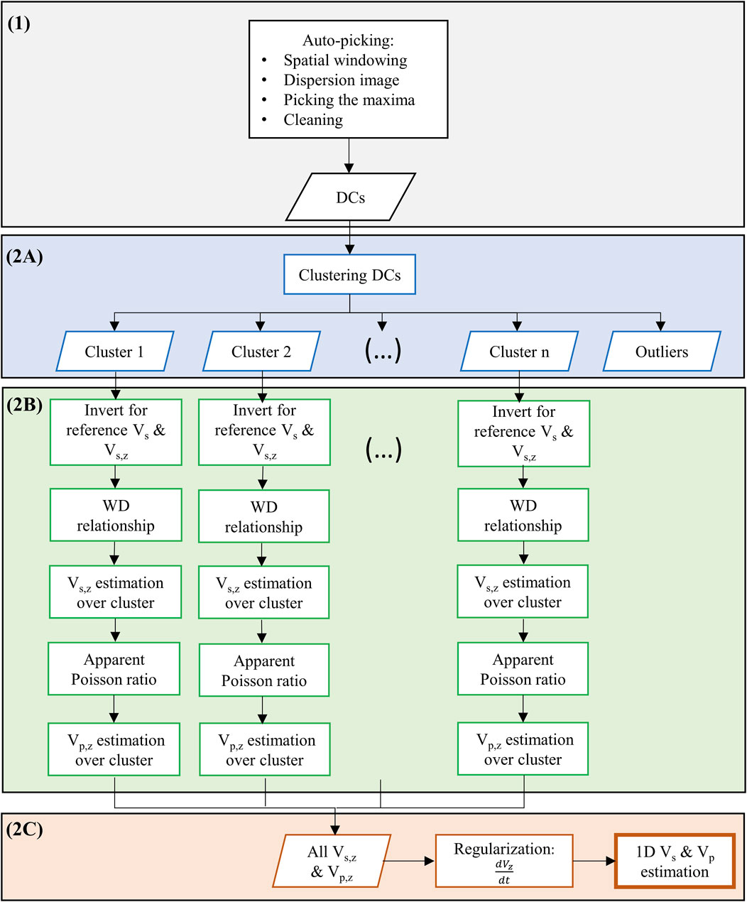
Figure 1. Workflow of the complete procedure of auto-picking and W/D transform. After the automatic DC extraction (1), the auto-picked DCs are grouped into clusters (2A). Then, for each cluster, the W/D method is applied (2B). Finally, (2C) the models of interval velocity V_s and V_p are estimated (modified from Khosro Anjom et al. (2019)).

Details are given below.

2.1 Automatic DC extraction

The auto-picking method used is based on the seminal work of Papadopoulou et al. (2021) with further developments aimed at improving the robustness and broadening the bandwidth of the extracted DCs (Zargar et al., 2023). The processing code is fully automatic and virtually applicable directly in the field.

The processing scheme is based on the definition of an appropriate spatial moving window that spans the seismic lines and computes the dispersion images based on the phase shift method (Park et al., 1998) at each position of the moving window and for several shot gathers in the same window (Papadopoulou et al., 2021; Zargar et al., 2023). The dispersion images of the different shots are stacked to improve S/N ratio and the DCs are automatically picked on each stacked spectrum. The auto-picking itself is based on the method developed by Papadopoulou (2021), which, after a preliminary picking, automatically selects the reliable branch of DCs on the basis of The DC is then automatically extended by picking additional points outside the main branch thanks to a series of quality controls (QCs). The required inputs beside the seismic records are the length of the moving window, the minimum and maximum source-receiver offset, and the shift of the moving window along the line. In the present processing scheme, a specific frequency band for the initial search of the maxima has to be set up by the operator.

2.2 Velocity estimation

We used the W/D method to directly transform the DCs into V_s and V_p models (Socco and Comina, 2017; Socco et al., 2017; Khosro Anjom et al., 2019; Khosro Anjom, 2021). The method is based on the strong correlation between DC in wavelength domain and time-average V_s (V_s,z) (Socco et al., 2017). The V_s,z at a certain depth $z$ is the weighted average velocity of the media from this depth up to the surface, which can be computed from the parameters of a layered V_s model using:

where ${\mathrm{V}}_{Si}$ and $h_i$ are the velocity and thickness of the $i$ th layer, respectively. The W/D relationship is based on the search for the wavelength at which the SW phase velocity is equal to the time-average velocity (V_s,z) at a certain depth. The W/D pairs define a relationship that represents the SW skin depth and that can be directly used to transform the DCs into V_s,z models. Since the skin depth of SW depends on the Poisson’s ratio (Pelekis and Athanasopoulos, 2011), Socco and Comina (2017) developed a method based on the sensitivity of the W/D relationship to estimate the time-average V_p (V_p,z) in addition to V_s,z. Based on the W/D data transform, Khosro Anjom et al. (2019) created a workflow to estimate interval V_s and V_p models that can be applied to laterally varying sites. The workflow for the estimation of V_s and V_p can be divided into three main steps (see Figure 1, blocks 2A, 2B, and 2C, respectively):

A. DCs clustering: the DCs of the seismic data set are grouped into clusters of homogenous sets by means of a hierarchical agglomerative clustering algorithm. The Euclidean distance is used as the metric to measure the dissimilarity of each two DCs, and average distance linkage criterion is considered to compute the distance between clusters (Khosro Anjom et al., 2019). Hierarchical clustering does not require information regarding lateral variation. The clusters can be obtained from the dendrogram plot or a distance threshold. The W/D transform is carried out separately for each cluster.

B. W/D transform: for each cluster, a reference DC based on the QC of Karimpour (2018) is selected. The reference DCs (one per cluster) are inverted using a Monte Carlo algorithm (Socco and Boiero, 2008) to estimate the reference V_s,z model (one per cluster). The reference V_s,z model and the reference DC are used to retrieve the reference experimental W/D relationship, which is used to transform the other DCs belonging to the same cluster. Then, from the W/D relationship of each cluster, a reference apparent Poisson’s ratio $\nu \left(z\right)$ is deduced (one per cluster). An apparent Poisson’s ratio is a property that relates the V_s,z and V_p,z models according to the following Eq. 2 (Socco and Comina, 2017):

The reference W/D relationship is applied to all DCs of the clusters to estimate the corresponding V_s,z models. Then, the estimated V_s,z models are transformed into V_p,z models thanks to the reference apparent Poisson’s ratio of the cluster.

C. Estimation of the interval velocities: the estimated V_s,z and V_p,z are transformed into interval V_s and V_p models using a DIX-type formula [i.e., inverse of Eq. (1)] (Dix, 1955). The DIX-type equation is sensitive to noise. To reduce the impact of the noise in the estimated V_s and V_p models, we impose the total variation regularization in the DIX-type equation (Khosro Anjom et al., 2019).

3 The case study

The investigated area is located in the Middle East, United Arab Emirates. The survey area is 300 m west away from the coastline, but the exact location of the survey area is kept confidential as requested by the data owner. On a geological standpoint, the survey area lies on the Cretaceous unit, as reported in the USGS geologic map (Pollastro et al., 1999). The geologic USGS province is called “Oman mountains”. The topography of the area is quite flat, and the ground surface is characterized by sand and gravel.

The data acquisition was carried out in 2020 for infrastructure development. The geophysical data set is composed of 5 m-spaced 45 parallel lines of seismic landstreamer and ERT data. The ERT data are not considered in this work.

The landstreamer data were acquired with a sledgehammer and plate as the source. The receiver was a 48-channel streamer with 1 m geophone spacing and a geophone frequency of 4.5 Hz. Each line was composed of 24 shot gathers (except for few lines with 22 shot gathers). The offset between the source and the 1^st geophone was 5 m and the streamer was shifted 5 m at every shot (between 2 and 5 stacks). The total length of the seismic line was 162 m for a total of 7.29 km for all 45 lines. The seismic acquisition layout is illustrated in Figure 2. The acquisition direction was from east (first geophone) to west (last geophone) and from south (first line L0) to north (last line L220). The profiles are oriented N80°W with respect to the geographical north. The area was also investigated with 8 cone penetration tests (CPTs) and 16 boreholes, whose locations are plotted in Figure 2.

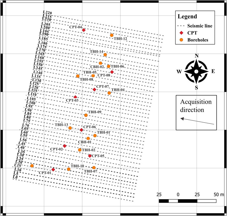
Figure 2. Overview of survey area: the 45 seismic landstreamer lines, the 8 CPTs and 16 boreholes. The acquisition direction was from east (first geophone) to west (last geophone) and from south (L0) to north (L220). The geographical coordinates are omitted on purpose as confidential.

The analysis of the 16 boreholes reveals the main geologic units of the area. The upper units are represented by gravelly, silty or shelly sand, while the deepest layers of the boreholes include breccia or gabbro, and sometimes calcarenite or sandstone. It is worth noting that below the geologic formation of (gravelly/silty/shelly) sand, the units of gabbro or breccia represent the outcropping bedrock. This clear discontinuity appears at a mean depth of 15 m from the top of the borehole, with a minimum depth of 8 m and a maximum depth of 23.5 m. Five out of 16 boreholes do not find the gabbro or breccia units, even though their well bottom is at a depth of around 20 m.

A representative example of the data set is shown in Figure 3, which represents a record for line L55, shot 4. This line was chosen as representative for the whole site and is shown later as it is close to CPT-02 and borehole TBH-02.

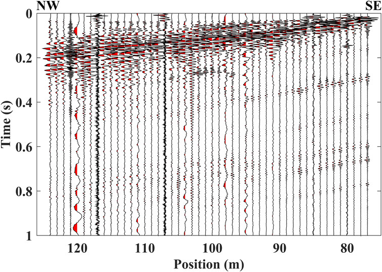
Figure 3. The data set. An example of recordings from line L55, shot 4.

4 Results

4.1 Auto-picking and comparison with manual picking

While the manual picking of landstreamer data is standardly carried out using the whole streamer (48 receivers and 47 m) and single source, for the auto-picking it is possible to select a smaller window, thus increasing the lateral resolution, and exploit several shots, thus increasing the S/N ratio. Moreover, the manual picking retrieves a DC every 5 m (which is the shift between neighboring positions of the shots), while for the auto-picking, thanks to its efficiency, a smaller shift of the window can be selected, down to the receiver spacing (1 m in this case). This provides a much denser DC data set. For the processing of the data, we chose a moving window of 24 receivers with a shift of 1 receiver (1 m) and stacking of 10 shots (offset from 5 to 50 m).

The manual and the auto-picking were carried out in Matlab proprietary codes using the phase shift method to compute the velocity spectra.

An example of the computed dispersion images for line L55 is depicted in Figures 4A, B with the picked DCs from the auto-picking code and manual approaches, respectively. Even though the general trends of the picked DCs are in good agreement, there are some differences. For instance, there are some discontinuities in the picked curve from the manual picking at around 40 Hz (Figure 4B) that are not present in the auto-picking method (Figure 4A). A possible reason for this slight discrepancy is that the dispersion images result from a different amount of input traces due to the moving window of the auto-picking method, which considered the traces coming from different shots.

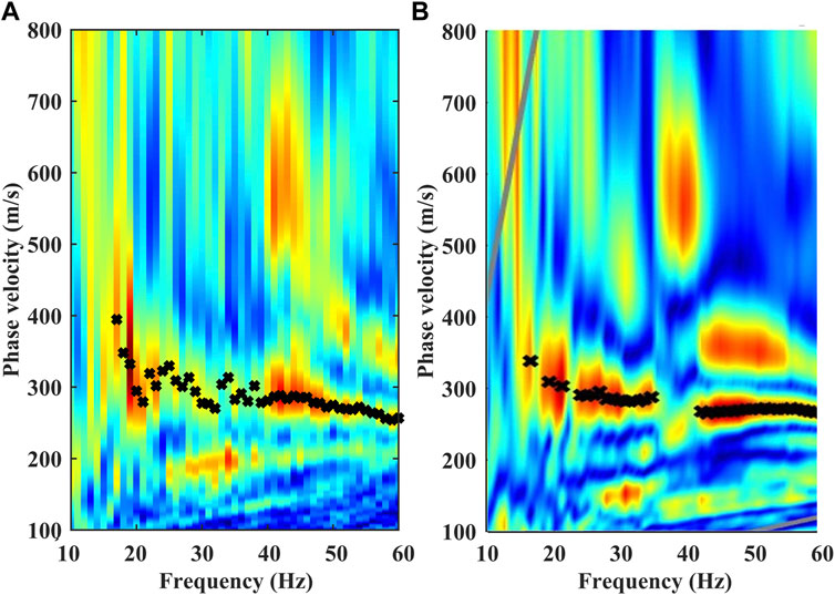
Figure 4. An example of DC extraction and the computed spectrum for line L55 from (A) the auto-picking code at the midpoint of around 30 m and from (B) the manual picking (shot 19, whose midpoint is 25.5 m). The red in the velocity spectrum means high amplitude, the blue means low amplitude.

The auto-picking method was applied to all 45 lines and more than 5,700 DCs were obtained, as shown in the pseudo-3D volume in Figure 5. The highest values of the phase velocity can be observed at large wavelength in the northwestern sector of the investigated area. The automatic DC extraction lasted less than 15 min with no need for any kind of user intervention. Figure 6 displays the extracted DCs from both auto-picking and manual picking as a function of wavelength for a representative line, L55. The data are represented with the horizontal axis of the receiver positions in descending order, while the direction of the acquisition goes from geographical southeast to northwest, as indicated in Figure 2. The extracted DCs from the auto-picking (Figure 6A) are denser in space since the spatial window moved every 1 m (i.e., the receiver spacing), while the DCs from the manual picking (Figure 6B) were estimated every 5 m (i.e., the shot spacing). Furthermore, the investigation depth of the DCs from the auto-picking (Figure 6A) is often higher than that from manual picking (Figure 6B), as can be observed from the wavelengths larger than 20 m.

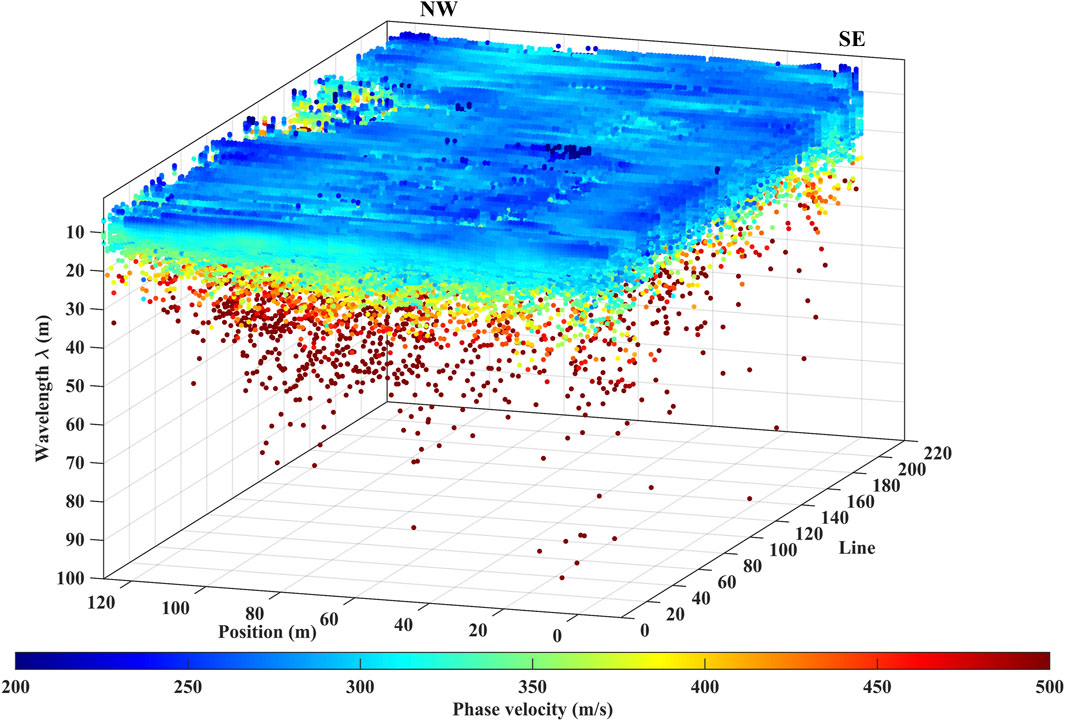
Figure 5. Pseudo-3D volume of the dispersion curves extracted with the auto-picking code.

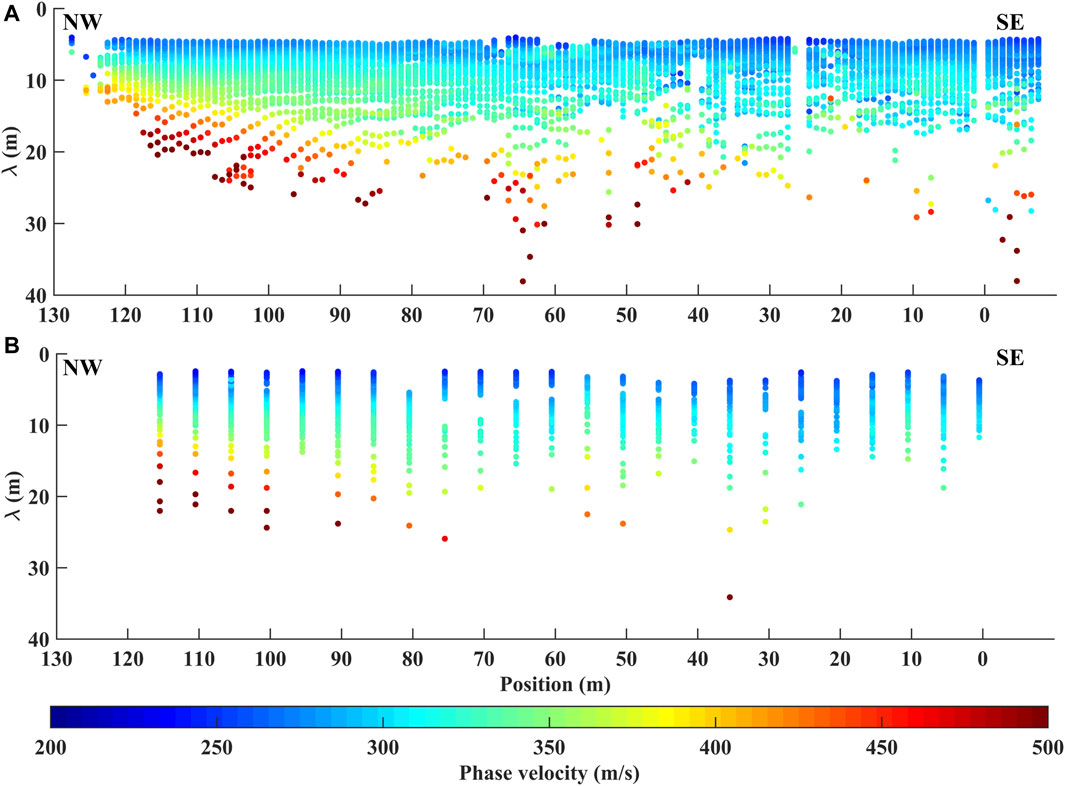
Figure 6. Pseudo-section of DCs obtained from auto-picking (A) and manual picking (B) for line L55.

The misfit between the DCs data points obtained from automatic and manual picking was calculated for all the lines. Given that the auto-picked DCs were more numerous than the manually picked DCs, the misfit was calculated for only the common frequency band of the DCs that had the same position. The average misfit for all the lines was −0.18%. The misfit distribution for line L55 is shown in Figure 7 as a bar chart. The average misfit is almost zero (−0.5%) and the standard deviation is 5.3%. The red curve represents the gaussian curve that fits the data.

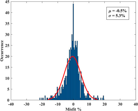
Figure 7. Distribution of the misfit between the DCs data points obtained from automatic and manual picking for line L55. The average of this distribution (µ) is −0.5% and the standard deviation (σ) is 5.3%. The red curve represents the gaussian that fits the bar chart of the data.

4.2 The final velocity models

The clustering of the estimated DCs through the auto-picking algorithm revealed three clusters (Figure 8). For each cluster, a reference DC was selected based on the QC and then inverted using the Monte Carlo algorithm to obtain the reference V_s,z model required for the W/D relationship. In Figure 9, we show the results of the Monte Carlo inversion, in which the three rows of plots refer to clusters 1, 2 and 3, respectively. The V_s and V_s,z models plotted in Figures 9B, C, E, F, H and I are depicted depending on the final misfit value, which is dimensionless: from the lowest misfit (purple lines) to the highest misfit (green lines). The reference DC of cluster 3 (Figure 9G) lacks low frequency data compared to the reference DC of clusters 1 and 2 (Figures 9A,D). As a result, the estimated W/D relationship and apparent Poisson’s ratio of cluster 1 and 2 cover more depth from the subsurface than cluster 3, as presented in Figure 10. The main reason behind this contrast in the investigation depth is the known outcropping hard rock formation in the western region of the site (cluster 3 in Figure 8). This outcrop formation guides the SWs to the shallow near-surface and prevents deep propagation, at least with the current acquisition settings.

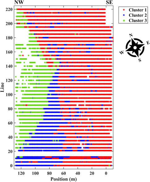
Figure 8. Map view of the spatial distribution of the auto-picked DCs and their clustering into three groups. The seismic lines are oriented N80°W.

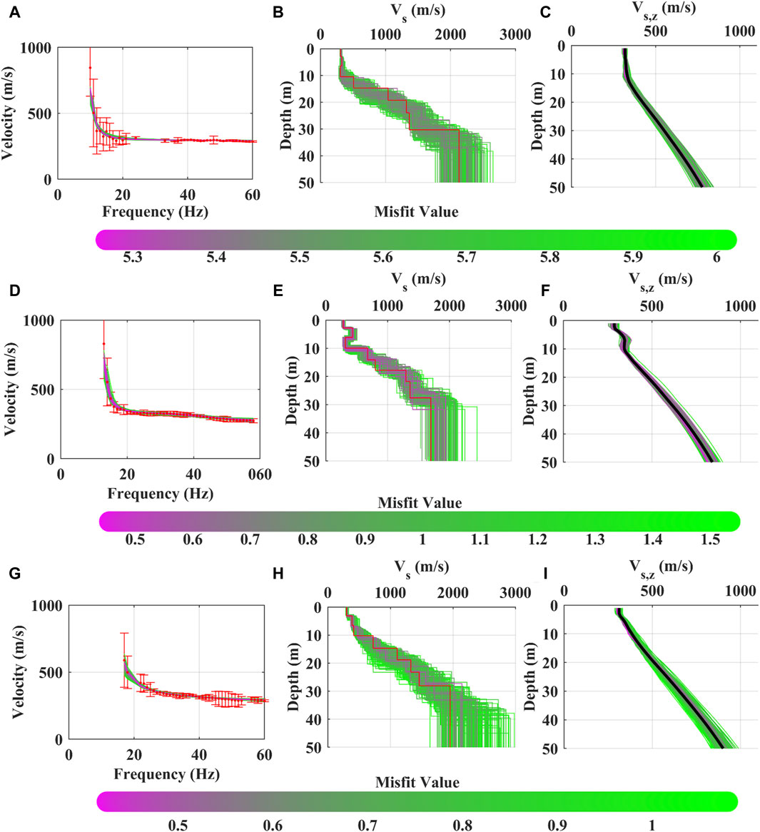
Figure 9. Results from MCI for the three reference DCs: (A) the reference dispersion curve for cluster 1, (B) the accepted V_s model for cluster 1, (C) time average V_s for cluster 1, (D) the reference dispersion curve for cluster 2, (E) the accepted V_s model for cluster 2, (F) time average V_s for cluster 2, (G) the reference dispersion curve for cluster 3, (H) the accepted V_s model for cluster 3, (I) time average V_s for cluster 3. The misfit value is dimensionless.

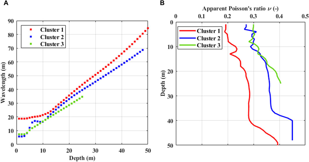
Figure 10. (A) The estimated W/D relationships for cluster 1 (red curve), cluster 2 (blue curve) and cluster 3 (green curve), (B) apparent Poisson’s ratio (ν) for the three clusters.

The estimated 1D V_s and V_p models from the W/D transform for all the DCs were merged and interpolated. In Figures 11A–C we show, respectively, a pseudo-3D volume of V_s, V_p, and Poisson’s ratio computed from the estimated models. The Poisson’s ratio shows high values above 0.4 at shallow depth in the northwestern region, in agreement with the known shallow water table at the site. The null Poisson’s ratios in Figure 11C are outliers, that are quite common in data transform and can be removed in a post-processing step.

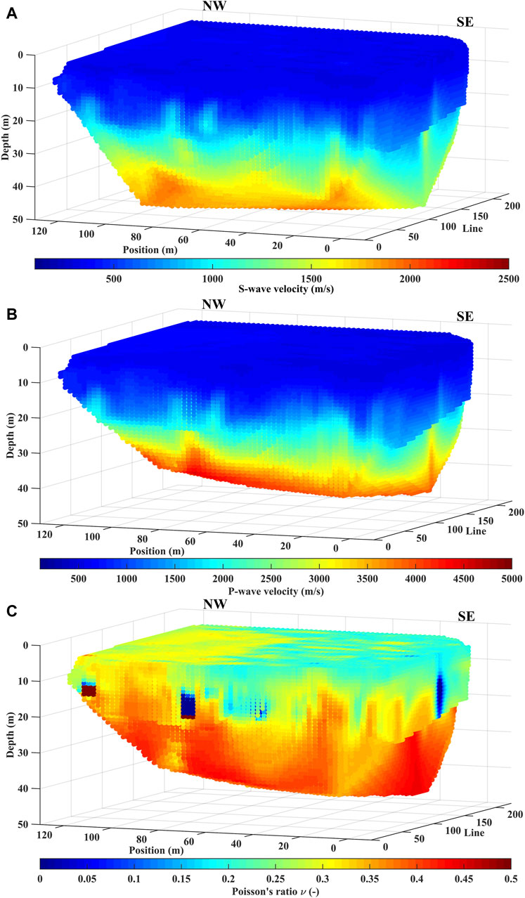
Figure 11. Pseudo-3D volume estimated using the W/D method: (A) V_s, (B) V_p, (C) Poisson’s ratio (ν).

5 Discussion

As regards the automatic extraction of the DCs, the results provide compelling evidence that the proposed method is valid and competitive. It is valid because the automatically picked DCs are highly comparable with the manually picked ones (see Figure 6), while it is competitive due to the exceptional time saving. In fact, the manual picking of the DCs would approximately require 2 h per line for a total of 90 h to retrieve around 1,000 DCs. This means around 5 min per DC, which can vary depending on the expertise level of the user. The auto-picking required 15 min to retrieve around 5,700 DCs, which means around 0.2 s per DC. This achievement may represent a major asset for both research and industrial projects dealing with large data sets and/or tight deadlines.

Thanks to the availability of CPTs and boreholes it was possible to assess the W/D method results.

The eight CPT soundings (see Figure 2) were used as benchmarks for the V_s models. As an example, we selected line L55 and CPT-02, which lies at around 72 m on the horizontal distance. Figure 12A shows the 2D section of the interval V_s superimposed on 1D V_s calculated from CPT data using the geotechnical parameters of the CPT (Robertson, 2009): $V_s={\left[{\alpha }_{Vs}\left(q_t-{\sigma }_V\right)/p_a\right]}^{0.5}$, where ${\alpha }_{Vs}$ is the V_s cone factor (dimensionless), $q_t$ is the total cone resistance (MPa), ${\sigma }_V$ is the in situ total vertical stress (MPa), $p_a$ is atmospheric pressure (MPa). In Figure 12, we compare the estimated V_s models from the W/D method and CPT. In Figure 12B, the solid black line is the interval V_s extracted at the correspondence of the location of CPT-02, while the dashed black line is the calculated V_s from CPT-02, that is, the same 1D V_s superimposed on the pseudo-section in Figure 12A. As a further validation, we compared the V_s trend with the available geological information from borehole TBH-02, which lies on line L55, only 22 m from CPT-02 (see Figure 2). We found that there is a geological discontinuity at a depth of 17.36 m (from ground surface), as can be seen from the stratigraphy depicted on the right of Figure 12B. The analysis of the lithology from TBH-02 revealed the presence of “medium dense, brown, silty, fine to medium sand” above the discontinuity. At depth 17.36–18 m there is “weak, grey to dark grey, thickly bedded, partially weathered gabbro”. At depth 18–19.4 m there is “light yellowish brown, matrix supported breccia”. Up to the borehole bottom of 20 m, there is “weak grey, weathered gabbro”. The depth of this geological discontinuity (17.36 m) approximately occurs in the depth range where the V_s approaches 1,500 m/s. This velocity value is in line with typical values of V_s for gabbro (Kearey et al., 2009). The lateral variation of V_s that can be observed from Figures 11A, 12A may have a major impact on the design of any engineering infrastructures, such as foundations.

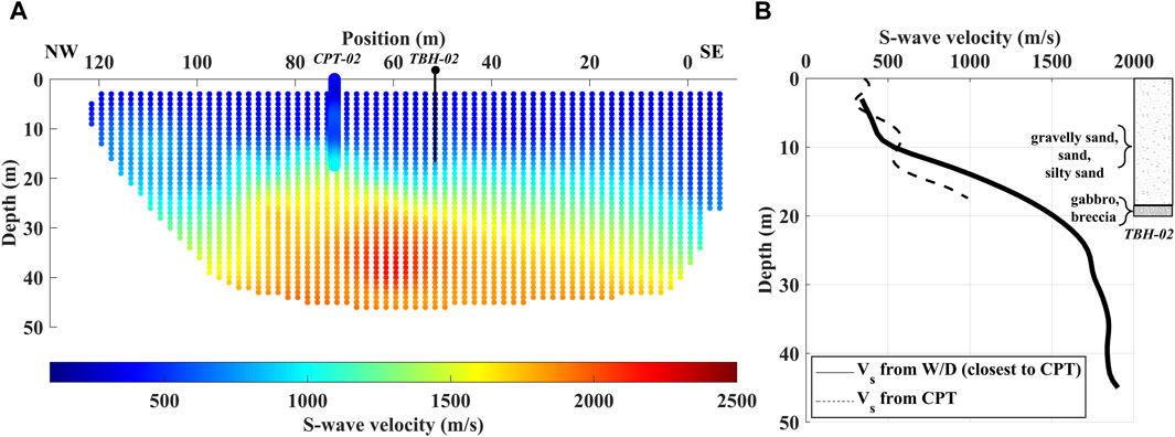
Figure 12. (A) Estimated interval V_s model (interpolated) for line L55 superimposed on the calculated V_s from CPT-02 (position ≈ 72 m); (B) comparison between the calculated V_s from CPT-02 (dashed black line) and the interval V_s extracted from the shot at the correspondence of CPT-02 (solid black line). On the right, the stratigraphy from borehole TBH-02.

The V_p obtained with the W/D method at line L55 was compared with the V_p model obtained through P-wave travel time tomography (Figure 13). Travel time data were inverted using the open-source Python package pyGIMLi (Rücker et al., 2017; Doyoro et al., 2022). The 2D refraction inversion is based on the shortest path method (Moser, 1991), includes topography and triangular mesh. The inversion of L55 ended after 8 iterations (around 10 min of total computation time). The initial chi-squared was 649, then it decreased to 10.4 after 8 iterations. The final relative root-mean-square error was 9.7% between the observed data and the calculated response.

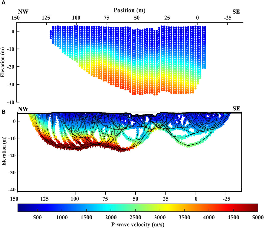
Figure 13. (A) Final interval V_p for one representative line (L55) after W/D method and (B) the V_p tomography after 2D travel time refraction inversion performed in pyGIML.i.

Figure 13A shows, for line L55, the 2D section of the interval V_p after W/D transform (interpolated), while Figure 13B plots the 2D model of V_p as computed in pyGIMLi. The models are not exactly compatible because pyGIMLi considers the true elevation of the receivers and the totality of the first breaks, while the W/D method considers the midpoints of the DCs, with topography added after the data transform to ease the comparison. However, both models show a significant increase in velocity (up to 5,000 m/s) at a distance between 70 and 100 m and at a depth from top of around 25 m (which is around −20 m of elevation in Figure 13). Moreover, at a distance of 80 m, the models show the same shape of the highest velocity deep interface related to the outcropping hard rock formation towards the northwest (right side of the graph). Finally, the V_p model obtained from the W/D method presents an investigation depth larger than that from travel time tomography.

We have demonstrated that the velocity models estimated with the W/D method are largely in agreement with available benchmarks from other methods, i.e., geotechnical data for the validation of V_s and geophysical inversion for the validation of V_p.

Regarding the time spent for the estimation of velocity models, this large data set required 1 workday for the estimation of reference W/D relationships and apparent Poisson’s ratios (steps 2A and 2B of the workflow in Figure 1) and around 30 min for the final estimation of V_s and V_p models (step 2C of Figure 1). A traditional DC inversion, for example, the laterally constrained inversion, would have required several days (up to a couple of weeks) to handle all the 5,700 DCs of our data set with powerful computational resources (Khosro Anjom et al., 2024) to produce V_s models. The first-break picking and the inversion in pyGIMLi (including topography and data formatting) to obtain V_p models took approximately half a workday per line, meaning around three working weeks for the whole data set.

6 Conclusion

We have presented a novel application of a semiautomatic approach to the analysis and processing of a large-scale landstreamer data set. The proposed workflow enables a fast estimation of the interval velocities V_s and V_p by means of automatic DC extraction (auto-picking), DCs clustering and W/D transform. It has been demonstrated that the combination of the auto-picking and W/D methods can be applied to fast seismic data processing and velocity estimation without the need for time-consuming data processing and inversion. What is further relevant is that the W/D transform allows the estimation of V_p models from surface waves with no need for first break picking and refraction inversion. We have demonstrated that the outcome from the proposed workflow is highly comparable with that from standard P-wave travel time tomography.

A crucial achievement was that the auto-picking of the DCs was more than 1,000 times faster than the standard manual picking. Moreover, the obtained models were supported by a dense data coverage and showed deeper investigation depth with respect to V_s obtained by manual DC picking and V_p obtained by travel time tomography.

This study represents the first application of such methodology to a data set which is composed of landstreamer data suitable for 3D interpretation. Automation and no need for inversion are the main benefits of the proposed workflow and truly represent a competitive asset in academic and company projects dealing with rapid deliverables of large amount of data. Besides, the short time required for data processing contributes to the added value of the work.

One possible limitation of the method adopted is that as W/D is a data transformation, the results are fully dependent on the data. The investigation depth depends on the retrieved wavelength of SW data and Poisson’s ratio.

The codes of the workflow are not available at this stage owing to further ongoing developments, but the workflow is clearly illustrated so that any researchers may have the opportunity code it.

Future work will consider further developments of the auto-picking method to enhance the level of automation and accuracy in the data processing. We expect the proposed method to open up research collaborations between academia and industry focusing on the robust and cost-effective processing of large seismic data sets.

Data availability statement

The original contributions presented in the study are included in the article, further inquiries can be directed to the corresponding author.

Author contributions

FP: Data curation, Supervision, Visualization, Writing–original draft, Writing–review and editing. FKA: Data curation, Methodology, Software, Visualization, Writing–original draft, Writing–review and editing. MK: Data curation, Methodology, Software, Visualization, Writing–original draft, Writing–review and editing. AB: Conceptualization, Writing–review and editing. YB: Data curation, Investigation, Writing–review and editing. HP: Investigation, Writing–review and editing. LVS: Conceptualization, Methodology, Supervision, Writing–review and editing.

Funding

The author(s) declare that financial support was received for the research, authorship, and/or publication of this article.

Acknowledgments

This study was carried out within the Ministerial Decree no. 1062/2021 and received funding from the FSE REACT-EU - PON Ricerca e Innovazione 2014–2020. The seismic landstreamer measurements of the case study were collected by Fugro Middle East. The authors would like to thank Fugro for providing access to the data. The authors want to thank François Janod (Fugro–France) for his helpful Matlab tool provided to pick the seismic data (Fugro MASW_Check^® code). Further thanks go to Florencia Balestrini (Fugro–The Netherlands) for her comments at the beginning of data analysis.

Conflict of interest

AB, YB, and HP were employed by the FUGRO.

The remaining authors declare that the research was conducted in the absence of any commercial or financial relationships that could be construed as a potential conflict of interest.

Publisher’s note

All claims expressed in this article are solely those of the authors and do not necessarily represent those of their affiliated organizations, or those of the publisher, the editors and the reviewers. Any product that may be evaluated in this article, or claim that may be made by its manufacturer, is not guaranteed or endorsed by the publisher.

References

Alyousuf, T., Colombo, D., Rovetta, D., and Sandoval-Curiel, E. (2018). Near-surface velocity analysis for single-sensor data: an integrated workflow using surface waves, AI, and structure-regularized inversion. Seg. Tech. Program Expand. Abstr. 2018, 2342–2346. doi:10.1190/segam2018-2994696.1
Bergamo, P., Boiero, D., and Socco, L. V. (2012). Retrieving 2D structures from surface-wave data by means of space-varying spatial windowing. GEOPHYSICS 77 (4), EN39–EN51. doi:10.1190/geo2012-0031.1
Cano, E. V., Akram, J., and Peter, D. B. (2021). Automatic seismic phase picking based on unsupervised machine-learning classification and content information analysis. GEOPHYSICS 86 (4), V299–V315. doi:10.1190/geo2020-0308.1
Colombo, D., Al-Najjar, M., Sandoval-Curiel, E., and Saad, R. (2017). Automatic near-surface velocity and statics by surface-consistent refraction analysis: application to a central Saudi Arabian megamerge. Soc. Explor. Geophys., 2671–2675. doi:10.1190/segam2017-17557867.1
Dix, C. H. (1955). Seismic velocities from surface measurements. GEOPHYSICS 20 (1), 68–86. doi:10.1190/1.1438126
Doyoro, Y. G., Chang, P.-Y., Puntu, J. M., Lin, D.-J., Van Huu, T., Rahmalia, D. A., et al. (2022). A review of open software resources in python for electrical resistivity modelling. Geosci. Lett. 9 (1), 3–16. doi:10.1186/s40562-022-00214-1
Foti, S., Hollender, F., Garofalo, F., Albarello, D., Asten, M., Bard, P.-Y., et al. (2018). Guidelines for the good practice of surface wave analysis: a product of the InterPACIFIC project. Bull. Earthq. Eng. 16 (6), 2367–2420. doi:10.1007/s10518-017-0206-7
Hjelm, L., Vosgerau, H., Smit, F. W. H., Nielsen, C. M., Gregersen, U., Rasmussen, R., et al. (2023). CCS2022-2024 WP1: the Stenlille structure. Seismic data interpretation mature potential Geol. storage CO2. doi:10.22008/GPUB/34661
Karimpour, M. (2018). Processing workflow for estimation of dispersion curves from seismic data and QC. Politecnico di Torino: M.SC.thesis.
Kearey, P., Brooks, M., and Hill, I. (2009). An introduction to geophysical exploration, 3. Blackwell Publ, Oxford.
Khosro Anjom, F. (2021). S-wave and P-wave velocity model estimation from surface waves. PhD thesis. Politecnico di Torino.
Khosro Anjom, F., Adler, F., and Socco, L. V. (2024). Comparison of surface-wave techniques to estimate S- and P-wave velocity models from active seismic data. Solid earth. 15 (3), 367–386. doi:10.5194/se-15-367-2024
Khosro Anjom, F., Teodor, D., Comina, C., Brossier, R., Virieux, J., and Socco, L. V. (2019). Full-waveform matching of VP and VS models from surface waves. Geophys. J. Int. 218 (3), 1873–1891. doi:10.1093/gji/ggz279
Malehmir, A., Heinonen, S., Dehghannejad, M., Heino, P., Maries, G., Karell, F., et al. (2017). Landstreamer seismics and physical property measurements in the Siilinjärvi open-pit apatite (phosphate) mine, central Finland. GEOPHYSICS 82 (2), B29–B48. doi:10.1190/geo2016-0443.1
McMechan, G. A., and Yedlin, M. J. (1981). Analysis of dispersive waves by wave field transformation. GEOPHYSICS 46 (6), 869–874. doi:10.1190/1.1441225
Moser, T. J. (1991). Shortest path calculation of seismic rays. GEOPHYSICS 56 (1), 59–67. doi:10.1190/1.1442958
Papadopoulou, M. (2021). Surface-wave methods for mineral exploration. PhD thesis. Politecnico di Torino.
Papadopoulou, M., Colombero, C., Staring, M., Singer, J., Eddies, R., Fliedner, M., et al. (2021). “Fast near-surface investigation with surface-wave attributes,” in NSG2021 2nd conference on Geophysics for infrastructure planning, monitoring and BIM. Presented at the NSG2021 2nd conference on Geophysics for infrastructure planning, monitoring and BIM (Bordeaux, France/ Online, France: European Association of Geoscientists & Engineers), 1–5. doi:10.3997/2214-4609.202120128
Park, C. B., Miller, R. D., and Xia, J. (1998). “Imaging dispersion curves of surface waves on multi-channel record,” in SEG technical program expanded abstracts 1998. Presented at the SEG technical program expanded abstracts 1998 (Society of Exploration Geophysicists), 1377–1380. doi:10.1190/1.1820161
Pelekis, P. C., and Athanasopoulos, G. A. (2011). An overview of surface wave methods and a reliability study of a simplified inversion technique. Soil Dyn. Earthq. Eng. 31 (12), 1654–1668. doi:10.1016/j.soildyn.2011.06.012
Pollastro, R. M., Karshbaum, A. S., and Viger, R. J. (1999). Maps showing geology, oil and gas fields and geologic provinces of the Arabian Peninsula (Open-File Report No. No. 97-470-B), Open-File Report. US Geological Survey.
Robertson, P. K. (2009). Interpretation of cone penetration tests — a unified approach. Can. geotechnical J. 46 (11), 1337–1355. doi:10.1139/T09-065
Rücker, C., Günther, T., and Wagner, F. M. (2017). pyGIMLi: an open-source library for modelling and inversion in geophysics. Comput. Geosciences 109, 106–123. doi:10.1016/j.cageo.2017.07.011
Socco, L. V., and Boiero, D. (2008). Improved Monte Carlo inversion of surface wave data. Geophys Prospect 56 (3), 357–371. doi:10.1111/j.1365-2478.2007.00678.x
Socco, L. V., and Comina, C. (2017). Time-average velocity estimation through surface-wave analysis: Part 2 — P-wave velocity. GEOPHYSICS 82 (3), U61–U73. doi:10.1190/geo2016-0368.1
Socco, L. V., Comina, C., and Khosro Anjom, F. (2017). Time-average velocity estimation through surface-wave analysis: Part 1 — S-wave velocity. GEOPHYSICS 82 (3), U49–U59. doi:10.1190/geo2016-0367.1
Van Der Veen, M., Spitzer, R., Green, A. G., and Wild, P. (2001). Design and application of a towed land-streamer system for cost-effective 2-D and pseudo-3-D shallow seismic data acquisition. GEOPHYSICS 66 (2), 482–500. doi:10.1190/1.1444939
Wang, Y., Liang, H., Rui, Y., Wang, S., Wang, J., and Sun, C. (2024). Near surface P-wave velocity inversion with average velocity analysis method. Chin. J. Geophys. 67 (3), 1208–1222. doi:10.6038/cjg2023R0029
Wang, Z., Sun, C., and Wu, D. (2021). Automatic picking of multi-mode surface-wave dispersion curves based on machine learning clustering methods. Comput. Geosciences 153, 104809. doi:10.1016/j.cageo.2021.104809
Zargar, A., Karimpour, M., and Socco, V. (2023). “Data driven auto-picking of surface wave dispersion curve,” in NSG2023 29th European meeting of environmental and engineering Geophysics. Presented at the NSG2023 29th European meeting of environmental and engineering Geophysics (Edinburgh, United Kingdom: European Association of Geoscientists & Engineers), 1–5. doi:10.3997/2214-4609.202320076
Keywords: MASW, surface waves, wavelength-depth transform, automatic picking, datadriven processing, landstreamer, seismic, geophysics-applied
Citation: Pace F, Khosro Anjom F, Karimpour M, Bolève A, Benboudiaf Y, Pournaki H and Socco LV (2024) Fast and semi-automatic S-wave and P-wave velocity estimations from landstreamer data: a field case from the Middle East. Front. Earth Sci. 12:1304593. doi: 10.3389/feart.2024.1304593
Received: 29 September 2023; Accepted: 04 April 2024;
Published: 24 April 2024.
Edited by:
Xintong Dong, Jilin University, ChinaReviewed by:
Zhi Wei, Peking University, ChinaBouhadad Youcef, National Earthquake Engineering Center (CGS), Algeria
Copyright © 2024 Pace, Khosro Anjom, Karimpour, Bolève, Benboudiaf, Pournaki and Socco. This is an open-access article distributed under the terms of the Creative Commons Attribution License (CC BY). The use, distribution or reproduction in other forums is permitted, provided the original author(s) and the copyright owner(s) are credited and that the original publication in this journal is cited, in accordance with accepted academic practice. No use, distribution or reproduction is permitted which does not comply with these terms.
*Correspondence: Francesca Pace, francesca.pace@polito.it