Combination prediction and error analysis of conventional gas production in Sichuan Basin

1 Introduction

Natural gas belongs to low-carbon fossil energy, with a strong development foundation and huge development potential. Moderately leveraging the unique advantages of clean, low-carbon, efficient, and stable natural gas can effectively promote the transformation and development of the energy system from fossil energy to renewable energy. Responding to the trend of international energy development, focusing on green energy and reducing carbon emissions (Shui. et al., 2022; Wang et al., 2023; Jia. et al., 2023). It can be seen that the reasonable and efficient exploration and development of natural gas is extremely important. To achieve this goal, accurately and stably predicting the trend of natural gas production changes has become an important link in development planning (Qiao. et al., 2020; Yuan. et al., 2022). Therefore, only by establishing a reliable prediction model and improving the accuracy of production prediction can we ensure the reasonable formulation of exploration and development planning plans.

Sichuan Basin has a long history of exploration and development, especially conventional gas has experienced multiple cycles of development, and is currently in the production growth period. In addition, there has been some research on methods and models for predicting natural gas production, and the most commonly used peak prediction methods and grey system methods have been well applied. For example, Chong et al. (2022) established an optimized grey system model with weighted score accumulation, using natural gas production in Germany, Italy, and Canada as examples to verify the feasibility of the model and apply it to study China’s natural gas production. The results indicate that this model is very suitable for predicting and analyzing natural gas production in China. Li. Xuemei et al. (2022a) proposed a grey prediction model combined with Particle swarm optimization, which can be used to predict time series with seasonal characteristics, with high prediction accuracy. The model was used to predict the quarterly production of natural gas in China from the third quarter of 2021 to the second quarter of 2024. The predicted results can provide a basis for formulating natural gas production plans and environmental policies. Wang. et al. (2016) used a multi cycle Hubbert model to predict China’s annual natural gas production based on several different ultimate recoverable reserve scenarios, and determined peak production, peak years, and future production trends. Accurate predictions of natural gas production and consumption can provide a basis for decision-making and help the government formulate new major policies.

Although these peak prediction models are also applicable to the production prediction of Sichuan Basin, due to the limitations of the models themselves, there are certain errors in the prediction results. In order to reduce the errors caused by the models, a combination model needs to be established. Qiao. et al. (2021) developed a combined model with automatic encoder and long-short-term memory, and calculated the difference between the US natural gas production and consumption as an example. The results indicate that the combined model outperforms other artificial intelligence models and has higher prediction accuracy. Research can provide reference for other time series predictions and natural gas policymakers. Tuan Hoang. et al. (2023) used three machine learning models, including decision tree, Random forest and support vector regression, to predict engine performance and emission parameters. In most cases, the accuracy rate was up to 99%. Therefore, using combination models for prediction can effectively combine the advantages of various prediction models, thereby improving the accuracy of prediction results.

Shapley value method is a good allocation method, which can reasonably allocate weights according to the error size of each model, and the established combination model often has higher accuracy (Cai. et al., 2023). Li et al. (2021) combined the individual characteristic weight coefficient with the Shapley value of each hydropower station, and proposed a variable coefficient Shapley value method for compensation benefit distribution of multi owner cascade hydropower stations. Taking China’s Nanhe Hydropower Station as an example, this method was compared with other typical distribution methods. The results show that the stability of this method in compensating benefit allocation is better than other methods, achieving fair and reasonable allocation of compensation benefits among cascade hydropower stations, and improving the utilization efficiency of water resources in the basin. An et al. (2019) combined the Shapley value method with network DEA to explore the problem of resource sharing and revenue allocation between different stages in a three-stage system. Several network DEA models have been established to calculate the optimal profits of the system before and after collaboration. In addition, the Shapley value was used to handle the problem of income distribution and verified through examples. Therefore, the Shapley value method can be combined with commonly used peak prediction models, such as the Hubbert model, Gauss model, etc., to establish a more accurate combination model for prediction results.

After the combination model is established, error analysis is required to study the accuracy and reliability of the model. Common error analysis methods include residual analysis and precision inspection, among which precision inspection includes F-test and t-test (Shichun et al., 2022; Pellatt. and Sun., 2023). Hong-Ju et al. (2022) established a model from 14 optimal wavelengths selected from KM spectrum, and tested whether the model has better performance in predicting Reducing sugar content. The F-test and t-test results of two samples further demonstrate the robustness and effectiveness of the model. Hong-Ju et al. (2023) realized rapid quantification and visualization of sweet potato starch content through near-infrared spectroscopy and image data fusion, and further verified the accuracy of the model through F-test and t-test. Therefore, after the residual analysis of the prediction results, the accuracy of the prediction results can be judged by combining the F-test and t-test.

According to the development of conventional gas production in Sichuan Basin, this paper firstly predicts conventional gas production by using Hubbert model, Gauss model and GM (1, N) model, and calculates the average percentage error of each model according to the prediction results. Then the Shapley value method is used to allocate the weight values of the three models. Based on the weight allocation results, a combination model for conventional gas production prediction is established, and the production prediction curves of the combination model and the single model are compared. Finally, residual analysis and accuracy testing were conducted on the prediction results of the four models, and the accuracy and reliability of each model were analyzed and studied (Liu et al., 2022; Liu et al., 2023a; Liu et al., 2023b).

2 Theory of combined prediction of natural gas production

2.1 Production prediction theory

2.1.1 Hubbert model

The Hubbert model is a widely used resource prediction method. The model was developed by geophysicist M King Hubbert proposed it in the mid-20th century (Nanzad. et al., 2017). The model can better simulate the changes in natural gas life cycle, namely the process of rapid growth, stable growth, and gradual decline after reaching the peak (Tunnell Bolorchimeg et al., 2021). In order to better predict the production trend of natural gas reserves, the ultimate recoverable reserve URR is introduced as a boundary constraint condition to improve the original Hubbert model. The improvement process is as follows.

Formula (1) is the famous Hubbert model. Among them, $Q\left(t\right)$ represents the cumulative production, the unit is ${10}^8{m}^3/a$; $N_R$ represents recoverable reserves, the unit is ${10}^8{m}^3/a$; $t$ is the production exploitation time, the unit is year; $t_m$ is the peak time of production; the unit is year; $k$ is the model parameter.

In formula (1), the traditional Hubbert model uses exploitable reserve $N_R$ for calculation, while in actual production, more consideration is given to the proved rate and recovery rate, and production planning is based on the ultimate recoverable reserves. Therefore, the ultimate recoverable reserves URR is introduced as the boundary condition, and the recoverable reserve $N_R$ is replaced by URR. Then, by taking the derivative of formula (1) over t, the calculation formula for annual production can be obtained, which is formula (2).

In the formula, $Q$ represents the annual production, the unit is ${10}^8{m}^3/a$.

When $t=t_m$, the production growth reaches its peak. At this point, the cumulative production $\mathrm{Q}\left(\mathrm{t}\right)$ has the highest rate of change, that is, $dQ\left(t\right)/dt$ is the largest. At this point:

In the formula, $Q_m$ represents the peak annual production, the unit is ${10}^8{m}^3/a$.

Transforming formula (3) into $URR=4Q_m/k$ and substituting it into formula (2) can obtain the annual production calculation formula for the Hubbert model, which is formula (4).

2.1.2 Gauss model

The Gauss model is similar to the Hubbert model in that it has the advantage of higher accuracy and is therefore equally suitable for natural gas production prediction research (Pan et al., 2019). The curves predicted using the Gauss model are often leaner and higher, but the overall trend of change is consistent with the Hubbert model from a macro perspective, and both exhibit symmetry with peak production as the axis of symmetry. The original expression of the Gaussian model is shown in formula (5).

In the formula, $\mu$ is the mean, $s$ is the standard deviation, and other parameters are the same as the Hubbert model.

In the process of natural gas extraction, the cumulative production within the $\left(0-\infty \right)$ interval of the extraction time $t$ is considered as the ultimate recoverable reserves URR. Replace $N_R$ in formula (5) with URR to obtain formula (6), which is the calculation formula for annual production $Q$.

Derive formula (6) from time $t$ to obtain the following expression.

When the production change reaches its highest value, the annual production change rate $dQ/dt=0$. At this point, the peak annual production time is:

Add $t_m=\mu$ Substitute it into formula (6) to obtain the annual peak production $Q_m$.

By substituting formulas (8), (9) into formula (6), the annual production calculation formula for the Gauss model can be obtained, which is formula (10), where $s$ is the model parameter.

2.1.3 GM (1, N) model

The grey model, abbreviated as the GM model, includes the GM (1, 1) model and GM (1, N) model. Due to its flexible and efficient advantages, it is also widely used in various predictions (Wang. et al., 2021). The GM (1, N) model represents a grey model established using first-order differential equations for n variables $x_1,x_2\dots x_n$. The traditional GM (1, N) method directly accumulates ${x_i}^{\left(0\right)}$ in the first order to generate a new sequence ${x_i}^{\left(1\right)}$, which is expressed in formulas 11, 12 (Sunil Kumar. et al., 2022).

Among them, $k=\mathrm{1,2}\dots p;i=\mathrm{1,2}\dots n$

Establish a simplified differential equation for GM (1, N) using the cumulative sequence ${x_i}^{\left(1\right)}$ to obtain a prediction model. After research, it was found that if there is a local numerical mutation in ${x_i}^{\left(0\right)}$, it will affect the overall accuracy of the prediction model (Ding. and Dang., 2023). Therefore, the correction weight coefficient $\alpha$ is introduced at the point of numerical mutation to reduce the prediction model error.

The corrected accumulation formula is:

Then, use sequence ${x_i}^{\left(1\right)}$ to establish a simplified differential equation and obtain formula (14).

The discrete format of the above equation can be rewritten as:

Based on the above algorithm, establish a GM (1, N) grey prediction model:

By using the GM (1, N) grey prediction model, a new sequence ${x_i}^{\left(1\right)}$ is obtained, and the sequence ${x_i}^{\left(0\right)}$ is obtained through first-order subtraction corrected by the weight coefficient $\alpha$.

2.2 Shapley value method combined prediction theory

Shapley value method is a method of interest distribution in cooperative Game theory, which can scientifically and fairly distribute the interests of each unit according to the degree of contribution, and obtain the weight value of each unit (Li et al., 2021). This allocation approach can be well reflected in combination prediction. When using Shapley values for weight allocation, all possible prediction models can be fully considered, and the greater the contribution of each model to the combination, the greater the final assigned weight. The process of determining weights and combining model formulas using the Shapley value method is as follows (Kjersti et al., 2021):

Suppose there are n prediction models, set $I=\left[1,2,3,\dots ,\mathrm{n}\right]$, and for any subset S of set I, its error is E (S). Let $e_i$ be the average percentage error of the ith prediction model, then the error E (S) of any subset S is:

In the equation, $\left|S\right|$ represents the number of predictive models in the set S.

The error allocation formula for the Shapley value method is:

Among them, $\omega \left(\left|S\right|\right)$ is the marginal contribution value of single prediction method i; $\left|S\right|$ is the number of single prediction methods in subset S; $E\left(S/i\right)$ is the absolute error value of subset S after removing i.

The weight formula of the ith prediction method in combination prediction is:

Among them, ${\omega }_i$ is the weight of the ith prediction method. Multiply each model with the weight and stack it to obtain the formula for the combined model:

Among them, $y_n$ represents the formula for each prediction model.

3 Combined prediction of conventional gas production

3.1 Single model production prediction

Sichuan Basin has a long history of conventional gas exploration and development, and the historical production is shown in Figure 1. Conventional gas has been in production since 1953 and has gone through three peaks by 2023, with each life cycle experiencing several stages of production increase, stable production, reaching peak, and decreasing production. This is similar to the prediction law of models such as Hubbert and Gauss.

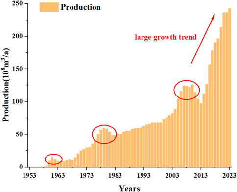
FIGURE 1. Historical production of conventional gas.

From Figure 1, it can be seen that the historical production of conventional gas has gone through three peak periods (circled in the figure). Since 2013, the production has rapidly increased, far exceeding the previous historical production (arrow in the figure). Therefore, it can be inferred that conventional gas production has entered a rapid production period and has entered the fourth production development cycle, which will reach its peak again in the future. In addition, it can be seen from the figure that the historical data for the fourth production development cycle is from 2013 to 2023. In order to verify the accuracy of the prediction results, half of the data was selected as the validation data, that is, from 2013 to 2017 as the historical data. Starting from 2018, the prediction was conducted, and the prediction results from 2018 to 2023 were compared with the historical data. Therefore, based on the data since 2013, three separate models were used to predict the trend of conventional gas production changes, and the weights of Shapley values were allocated according to the errors, ultimately forming a combined prediction.

Before the single model prediction of conventional gas production, the numerical range of the ultimate recoverable reserves URR should be estimated first. The following is a simple estimation of URR through numerical calculation. Through geological exploration, it is found that the conventional gas resource in Sichuan Basin is $12.23\times {10}^{12}{m}^3$. Then, by analyzing the exploration and development laws of many gas reservoirs in the Sichuan Basin, the range of conventional gas proved rate and recovery factor is selected. According to the current technical conditions for conventional gas exploration and production in Sichuan Basin, the proven rate of conventional gas is 40%–60%, that is, the cumulative proven reserves at the end of the life cycle range from $\left(4.892-7.338\right)\times {10}^{12}{m}^3$. At present, the recovery factor of conventional gas in Sichuan Basin is about 40%, so the estimated range of URR is $\left(19568-29352\right)\times {10}^8{m}^3$.

From Figure 1, it can be seen that the growth stage of conventional gas production began in 2013. In order to test the accuracy of the prediction results, data from (2013–2017) was chosen as the basis for prediction, and the middle value of the URR range was used as the final recoverable reserves for production prediction (taking URR = 25,000 $\times {10}^8{m}^3$). Then, the Hubbert model, Gauss model, and GM (1, N) model were used to predict the changes in conventional gas production starting from 2018. Finally, the data from 2018 to 2023 in the prediction results were compared with historical data to determine the accuracy of the prediction results.

Figure 2A shows URR = 25,000 $\times {10}^8{m}^3$, the conventional gas production prediction results of the Hubbert model, Gauss model, and GM (1, N) model are obtained. To study the general pattern of natural gas production growth and maintain the symmetry of the prediction model, the prediction time is only truncated to 2080, making it easier to observe the differences in the trend of the three models’ prediction curves. From Figure 2A, it can be seen that the faster the growth rate of production, the higher the peak production, and the faster the rate of decline, resulting in lower production during the decline period.

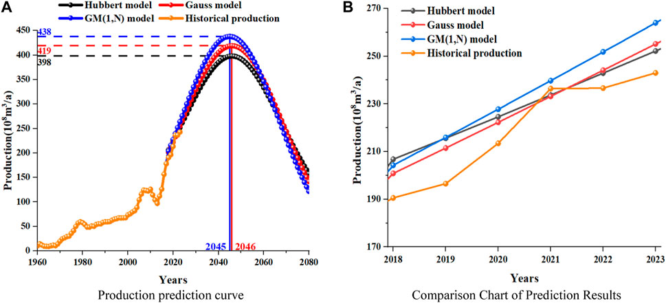
FIGURE 2. Prediction results of conventional gas production.

The production time relationship obtained from the formula in Section 2.1 is as follows. Among them, formula (26) is the production time relationship of the Hubbert model, formula (27) is the production time relationship of the Gauss model, and formula (28) is the production time relationship of the GM (1, N) model.

From Figure 2A, it can be seen that the trends predicted by the Hubbert model and Gauss model are consistent, reaching their peak in 2046, with peak production of 398 $\times {10}^8{m}^3$ and 419 $\times {10}^8{m}^3$, respectively; The GM (1, N) model has a faster growth rate, an earlier peak time of 2045, a larger peak production of 438 $\times {10}^8{m}^3$, and a faster decline rate in the GM (1, N) model.

Figure 2B shows a comparison between the predicted results of the three models from 2018 to 2023 and historical data. From the figure, it can be preliminarily seen that among the three prediction models, the GM (1, N) model has a relatively larger prediction error. The error analysis of the three models over the past 6 years is obtained by calculating the production error, as shown in Table 1.

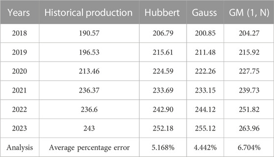
TABLE 1. Error analysis of prediction results in the last 6 Years.

According to Table 1, comparing the average percentage error of the three prediction models, the Gauss model has the highest prediction accuracy with an error of 4.442%, followed by the Hubbert model with an error of 5.168%, and the GM (1, N) model with the worst accuracy with an error of 6.704%. In order to improve the accuracy of prediction models and effectively combine the advantages of different prediction models, the Shapley value method is used to allocate the weights of the three prediction models, forming a combined prediction model.

3.2 Combined model production prediction

According to the error results obtained in 3.1, the total average percentage error is E = (5.168 + 4.442 + 6.704)/3 = 5.438 (unit is %, and in subsequent calculations, the error units are %). According to the Shapley value method, let the set I = (Shui. et al., 2022; Wang et al., 2023; Jia. et al., 2023) represent the three prediction models, and then, according to formula (21), the error values E (S) of all subsets of the combined model can be obtained, as shown in Table 2.

TABLE 2. Subset error table.

According to the method in Section 2.2, the Shapley values of the three models can be obtained according to formula (22) as follows: E1 = 1.610, E2 = 1.066, E3 = 2.762. At this point, E1 + E2 + E3 = 5.438, that is, the sum of the three values is equal to the average percentage error, indicating that the calculation results are correct. Then use formulas 23, 24 to calculate the weight values of the three prediction methods in the combined prediction, ${\mathrm{\omega }}_1=0.352$, ${\mathrm{\omega }}_2=0.402$, ${\mathrm{\omega }}_3=0.246$, it can be concluded that the combined prediction model is:

The combination prediction model is shown in formula (29). Among them, Q represents the production predicted by the combination model, and Q1, Q2, and Q3 represent the production predicted by the Hubbert model, Gauss model, and GM (1, N) model, respectively. Below, the conventional gas production is predicted based on the combination model, and the results obtained are shown in Table 3.

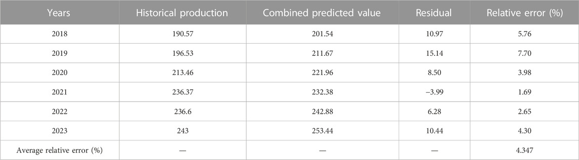
TABLE 3. Error analysis of combined prediction results.

From Table 3, it can be seen that the combination model established based on the Shapley value method has higher accuracy, with an average relative error of only 4.347%. Among the prediction results in the past 6 years, the relative error was relatively large only in 2019, and the prediction results in other years were relatively close to historical values, with the minimum error of 1.69%.

Figure 3A shows the proportion of errors among different prediction models, representing the relative proportion of prediction results errors among the four models from 2018 to 2023. From the graph, it can be seen that the error between the Hubbert model and the GM (1, N) model is relatively large, while the Gauss model and the combination model predict results more accurately. Figure 3B shows a comparison of the average errors of the four models. From the graph, it can be seen that the average error of the combined model is lower than that of any other model. Therefore, the combined model is more accurate than the single model.

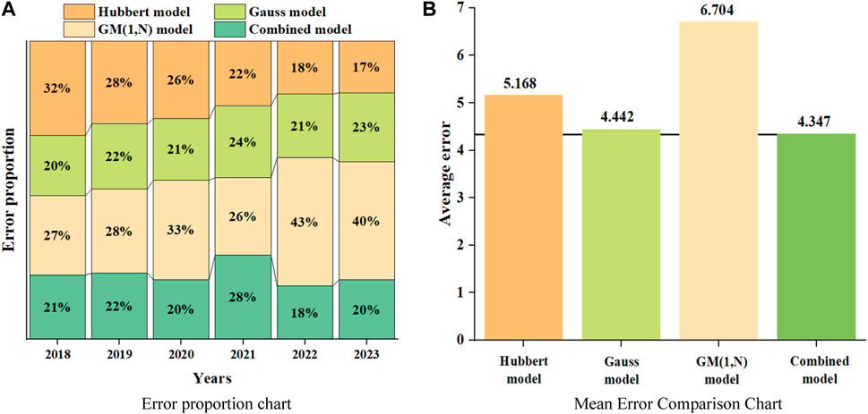
FIGURE 3. Comparison of errors among different models.

Next, starting from 2015, for the new life cycle of conventional gas production, the results predicted by the combined model and other single models are compared, as shown in Figure 4. The curve section in the figure from 2015 to 2017 is historical data, and the production forecast results start from 2018. The two figures in Figure 4 contain the prediction curves of three single models, of which Figure 2A is to show the stable production period under the prediction of the three models, and Figure 2B is to compare the prediction results of the combined model with those of other models. It is easier to observe and compare the two figures.

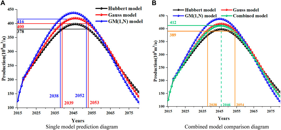
FIGURE 4. Comparison of results of different models.

Based on Figures 2A, 4A, it can be seen that when using the Hubbert model and Gauss model separately for production prediction, conventional gas production will reach its peak in 2046, with peak production of 398 $\times {10}^8{m}^3$ and 419 $\times {10}^8{m}^3$, respectively, with a stable production period of (2039–2053) years, a stable production period of 15 years. When using the GM (1, N) model for production prediction, conventional gas production will peak in 2045, with a peak production of 438 $\times {10}^8{m}^3$, with a stable production period of (2038–2052) years, a stable production period of 15 years.

From Figure 4B, it can be seen that when using the combined model for production prediction, the conventional gas production will reach its peak in 2046, with a peak production of 412 $\times {10}^8{m}^3$, a stable production period of (2038–2054), a stable production period of 17 years, and a stable production of 389 $\times {10}^8{m}^3$. It can be seen that the prediction results of the combined model have a longer stable production period, and its production prediction curve is similar to the results of the Gauss model, but the trend of production change is more stable.

4 Error analysis of prediction results

According to the contents in Section 3.2, the prediction results of the combined model are more accurate than those of any single model, and the predicted curve is more stable, with a higher stable production period. Next, from the perspective of residual analysis and precision test, the prediction results are compared with the standardized residual to determine the stability and accuracy of the prediction model, and then the F-test and t-test are used to determine the reliability of the prediction model.

4.1 Residual analysis

Residual can effectively reflect the deviation between the predicted value and the actual value, thus intuitively comparing the accuracy of the prediction model. Standardized residual can reflect the stability and correctness of the prediction results. Generally, standardized residual is within the range of [−2, 2] (Mohammed and Muhammad, 2021). If it exceeds the range, it indicates that the predicted results are incorrect. The calculation formula for residual and standardized residual is as follows.

In the equation, ${\delta }_i$ is the residual, $Y_i$ is the predicted production value, $y_i$ is the actual production value, ${\delta }_i^{*}$ is the standardized residual, $\overline{\delta }$ is the average residual value, $\sigma$ is the residual standard deviation.

Due to the possibility of randomness in a single calculation, in order to reduce errors caused by accidental results, and to demonstrate that slight fluctuations in URR have no impact on the predicted results. Take a fluctuation of around 5% for URR, when the URR = 25,000 $\times {10}^8{m}^3$, take a fluctuation range of ±1,000 $\times {10}^8{m}^3$, that is, let the URR fluctuate randomly within the range of (24,000–26000) $\times {10}^8{m}^3$, then use a single model and a combined model to predict the conventional gas production for 10 times respectively, and finally carry out residual processing on the results obtained, and analyze the error degree of the model, as shown in Figure 5.

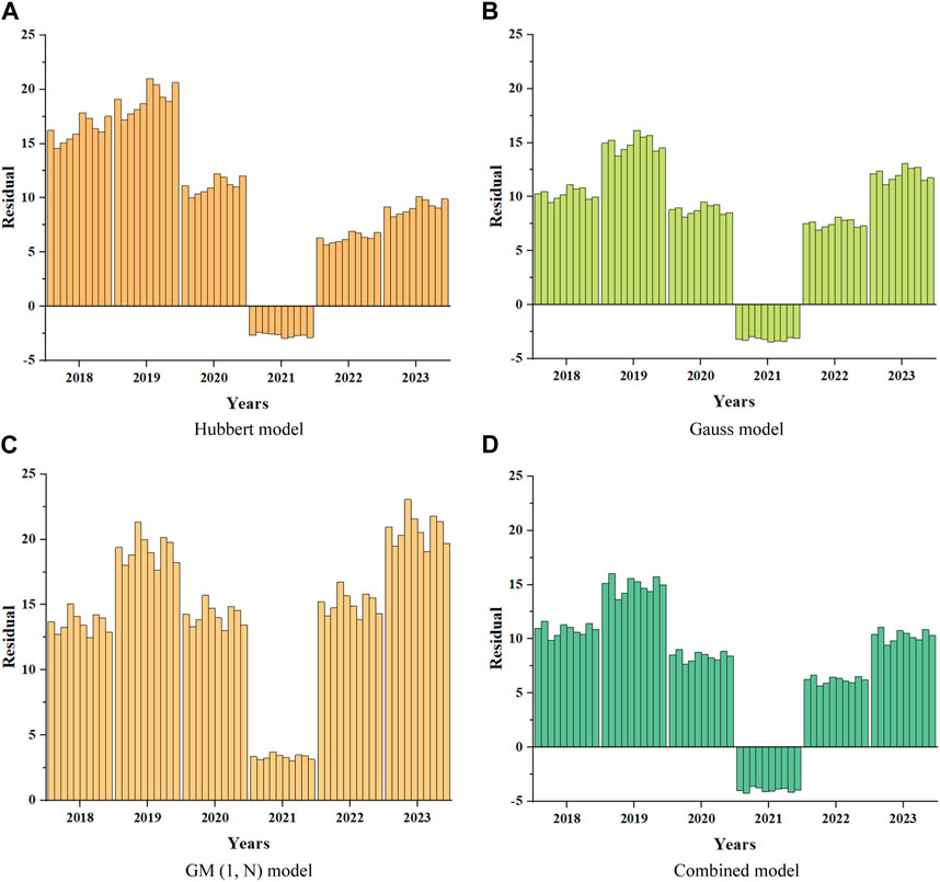
FIGURE 5. Residual results of different models.

Figure 5 shows the residual results of 10 predictions of conventional gas using four models. Through comparison, it can be concluded that the GM (1, N) model has the highest degree of error, with residual values generally above 10 except for 2021. Overall, the residuals of the Hubbert model are relatively large, while the residuals of the Gauss model and the combined model are relatively small and stable, with residuals basically maintained between 5 and 10, and only the predicted residuals in 2019 are relatively large. Therefore, it can be preliminarily determined that among the four models, the Gauss model and the combined model have relatively high accuracy.

Below, based on the production results calculated in Section 3, the residuals and standardized residuals of the four models are compared, as shown in Figure 6.

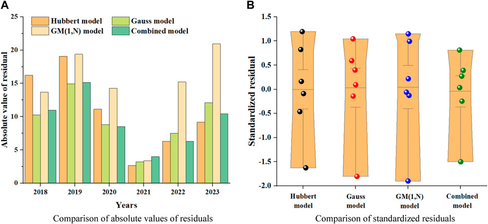
FIGURE 6. Comparison of residuals.

For the convenience of comparison, the residuals are taken as absolute values, as shown in Figure 6A. For the four prediction models, the Gauss model and the combined model have the highest accuracy. In the early stages of prediction, the Gauss model has higher accuracy, but over time, the accuracy of the combined model gradually exceeds that of the Gauss model.

Figure 6B shows a comparison of standardized residuals for four prediction models. Firstly, all standardized residuals are within the range of [−2, 2], indicating that there will be no errors in using these models for prediction, but there may be some errors. The closer the standardized residual is to 0, the more stable the predicted results are and there will be no significant fluctuations. From the graph, it can be seen that the standardized residual range of the combined model is the smallest, and almost all of them are concentrated around 0, indicating that the stability of the combined model is the best. When using the combined model for prediction, the overall results will not fluctuate too much.

Therefore, based on the results of the entire residual analysis, the combined model has the best accuracy and stability in predicting conventional gas production.

4.2 Accuracy inspection

To ensure the accuracy of the results, the precision of the results should also be analyzed, which requires precision testing of the predicted results. Therefore, for production data obtained from different prediction models, precision validation should be conducted first. If there is no significant difference, accuracy validation should be conducted again. In this case, F-test and t-test are required.

The F-test is to determine whether there is a significant difference in the prediction results and whether the precision meets the requirements by comparing the deviation between the predicted value and the actual value. The main method is to calculate the F-value, then determine the confidence interval, consult the critical value table of F-test, and judge whether there is significant difference by comparing the size relationship between the F-calculation and the F-table.

The calculation method of F value is shown in formula (32) (Li. Aimin et al., 2022). Among them, $S_1^2$ and $S_2^2$ represent the larger and smaller variances in the predicted and actual values, respectively.

The t-test method calculates the t-value based on the arithmetic mean, variance, and number of data between the predicted and actual values, and then determines the confidence interval. The critical value table of the t-test is compared, and the reliability of the calculation results is determined by comparing the size relationship between the t-calculation and the t-table, thereby indicating whether the selected prediction method is reliable. In addition, F-test is the premise of t test, and t test can be continued only when the conditions of F-test are met.

The calculation method of t value is shown in formula (33) (Delacre et al., 2022). Among them, $\overline{X}$ is the arithmetic mean, S² is the variance, and n is the number of data.

The predicted results and historical production data of the four models are shown in Table 4.

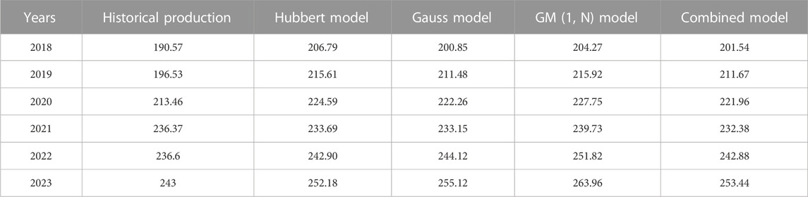
TABLE 4. Production data for the last 6 Years.

First, carry out F-test for the four models, and calculate the F-value according to formula (32).

Among them, $S_{history}^2$ is the variance of historical data, $S_{Hubbert}^2$ is the variance of Hubbert model prediction results, $S_{Gauss}^2$ is the variance of Gauss model prediction results, $S_{GM\left(1,N\right)}^2$ is the variance of GM (1, N) model prediction results, and $S_{combination}^2$ is the variance of combination model prediction results.

The confidence interval of 95% was selected. According to the critical value table of F-test, F-table = 3.217, and the size relationship between the F-calculation and F-table was compared. If F-calculation is greater than F-table, it indicates that there is no significant difference in the predicted values, and t-test can be continued. If the F-calculation is less than the F-table, it indicates a significant difference between the predicted values, and this prediction method cannot be adopted, and there is no need to continue with t-test. It is found that the F-values of the four models are less than the critical value of the F-test, which indicates that there is no significant difference between the precision of the prediction results of the four models. Therefore, the accuracy test can be continued.

Perform t-tests on each of the four models and calculate the t-value according to formula (33). Due to the use of production data from the past 6 years and the comparison between predicted and historical values, the degree of freedom in t-test is f = n₁ + n₂-2 = 6 + 6–2 = 10. Among them, n₁ and n₂ are the number of predicted production and historical production, both of which are 6.

Among them, $\overline{X_{history}}$ is the mean of historical data, $\overline{X_{Hubbert}}$ is the mean of Hubbert model prediction results, $\overline{X_{Gauss}}$ is the mean of Gauss model prediction results, $\overline{X_{GM\left(1,N\right)}}$ is the mean of GM (1, N) model prediction results, and $\overline{X_{combination}}$ is the mean of combination model prediction results.

Select a confidence interval of 95% and look up the t-test threshold table, which shows that t-table = 1.812. Comparing the calculation results, it can be seen that t₁>t-table and t₃ > t-table. Therefore, the prediction results obtained using the Hubbert model and GM (1, N) model do not have sufficient precision and have significant errors. In addition, t₄ < t₂, compared to the Gauss model, the t-value of the combined model is smaller, indicating that the prediction results obtained by the combined model have higher precision.

Therefore, based on the overall accuracy test results, the accuracy and precision of the prediction results are the best when using a combination model for conventional gas production prediction.

4.3 Comprehensive evaluation

After the residual analysis and precision test of the prediction results of the combined model and the single model, the following conclusion are obtained.

Among the four models, GM (1, N) model has the largest error in prediction results and the largest range of error fluctuations. The Hubbert model also has a larger error in prediction results and a larger range of error fluctuations. Moreover, the precision of these two models is not enough. After F-test and t-test, significant deviation is found in the prediction results, which indicates that GM (1, N) model and Hubbert model are not reliable for prediction.

The error of the Gauss model and the combined model is relatively small, but the error fluctuation of the combined model is smaller, indicating that when using the combined model for prediction, the results are more stable. At the same time, through accuracy testing, it was found that both models have high precision and the methods are reliable. However, the t-value of the combined model is smaller, indicating that its accuracy is higher.

In conclusion, compared with a single model, the most accurate and stable prediction model is the Gauss model. However, after the weight distribution of the three models using the Shapley value method, the combined model obtained has higher accuracy and stability, which indicates that the combined model has better prediction effect on conventional gas production.

5 Conclusion

This article uses the Shapley value method to allocate the weight values of three commonly used models for natural gas production prediction. Based on the average error of the three models’ predictions, the weights of each model are obtained, and a combined prediction model is established. The rules of the production prediction curves of different models are analyzed, and residual analysis and accuracy testing are conducted on the prediction results. The accuracy and reliability of the prediction models are compared, and the conclusion are as follows.

1) Shapley value method can effectively reduce the errors caused by the shortcomings of a single model. After weight allocation and the formation of a new combined model, it can effectively combine the advantages of each model and improve the accuracy of prediction. The comparison of the average error shows that the error of the combined model is lower than that of any single model, indicating that its accuracy is the highest. After the residual analysis and precision test of the prediction results of the four models, it is found that the combined model meets the F-test and t-test, with the smallest test value and the highest precision, and the residual and standardized residual are lower than other models, which indicates that the combined model has the highest accuracy and the most reliable method.

2) Using a combined model to predict conventional gas production, the results show that conventional gas production will peak in 2046, with a peak production of 412 $\times {10}^8{m}^3$, a stable production period of (2038–2054), a stable production period of 17 years, and a stable production of 389 $\times {10}^8{m}^3$. The prediction results of the combined model have a longer stable production period and a more stable trend in production changes.

Data availability statement

The raw data supporting the conclusion of this article will be made available by the authors, without undue reservation.

Author contributions

HL: Conceptualization, Data-curation, Methodology, Supervision, Writing–review and editing. GY: Conceptualization, Data-curation, Methodology, Supervision, Writing–review and editing. YaC: Formal Analysis, Project administration, Validation, Writing–review and editing. YF: Formal Analysis, Project administration, Validation, Writing–review and editing. YuC: Investigation, Writing–original draft, Writing–review and editing, Conceptualization. DZ: Investigation, Writing–original draft, Writing–review and editing, Conceptualization.

Funding

This study was financially supported by Sichuan Science and Technology Program: 2021JDR0401.

Conflict of interest

Authors HL, YC YF, and GY was employed by the PetroChina Southwest Oil and Gas Field Company.

The remaining authors declare that the research was conducted in the absence of any commercial or financial relationships that could be construed as a potential conflict of interest.

Publisher’s note

All claims expressed in this article are solely those of the authors and do not necessarily represent those of their affiliated organizations, or those of the publisher, the editors and the reviewers. Any product that may be evaluated in this article, or claim that may be made by its manufacturer, is not guaranteed or endorsed by the publisher.

References

An, Qingxian., Wen, Yao., Ding, Tao., and Li, Y. (2019). Resource sharing and payoff allocation in a three-stage system: integrating network DEA with the Shapley value method. Omega 85, 16–25. doi:10.1016/j.omega.2018.05.008
Cai., Wenqi, Bahari Kordabad., Arash, and Gros., Sébastien (2023). Energy management in residential microgrid using model predictive control-based reinforcement learning and Shapley value. Eng. Appl. Artif. Intell. 119, 105793. doi:10.1016/j.engappai.2022.105793
Chong, Liu., Lao., Tongfei, Wu., Wen-Ze, Xie, W., and Zhu, H. (2022). An optimized nonlinear grey Bernoulli prediction model and its application in natural gas production. Expert Syst. Appl. 194, 116448. doi:10.1016/j.eswa.2021.116448
Delacre, Marie., Lakens, Daniel., and Leys, Christophe. (2022). Why psychologists should by default use welch's t-test instead of student's t-test. Int. Rev. Soc. Psychol. 35, 1–3. doi:10.5334/irsp.613
Ding., Yuanping, and Dang., Yaoguo (2023). Forecasting renewable energy generation with a novel flexible nonlinear multivariable discrete grey prediction model. Energy 277, 127664. doi:10.1016/j.energy.2023.127664
Hong-Ju, He., Wang., Yangyang, Zhang., Mian, Wang, Y., Ou, X., and Guo, J. (2022). Rapid determination of reducing sugar content in sweet potatoes using NIR spectra. J. Food Compos. Analysis 111, 104641. doi:10.1016/j.jfca.2022.104641
Hong-Ju, He., Wang., Yuling, Wang., Yangyang, Al-Maqtari, Q. A., Liu, H., Zhang, M., et al. (2023). Towards rapidly quantifying and visualizing starch content of sweet potato [Ipomoea batatas (L) Lam] based on NIR spectral and image data fusion. Int. J. Biol. Macromol. 242, 124748. doi:10.1016/j.ijbiomac.2023.124748
Jia, G., Lei, M., Li, M., Xu, W., Li, R., Lu, Y., et al. (2023). Hydrogen embrittlement in hydrogen-blended natural gas transportation systems: a review. Amsterdam, Netherlands: International Journal of Hydrogen Energy.
Kjersti, Aas., Martin, Jullum., and Anders, Løland. (2021). Explaining individual predictions when features are dependent: more accurate approximations to Shapley values. Artif. Intell. 298, 103502. doi:10.1016/j.artint.2021.103502
Li, Wang., Yinghai, Li., Wang., Yongqiang, Guo, J., Xia, Q., Tu, Y., et al. (2021). Compensation benefits allocation and stability evaluation of cascade hydropower stations based on Variation Coefficient-Shapley Value Method. J. Hydrology 599, 126277. doi:10.1016/j.jhydrol.2021.126277
Li., Aimin, Huang., Xiaolan, Ling, Yan., and Cheng, J. (2022b). Pseudo-template molecularly imprinted polymeric fiber solid-phase microextraction coupled to gas chromatography for ultrasensitive determination of 2,4,6-trihalophenol disinfection by-products. J. Chromatogr. A 1678, 463322. doi:10.1016/j.chroma.2022.463322
Liu, Y. B., Lebedev, M., Zhang, Y. H., Wang, E. Y., Li, W. P., Liang, J. B., et al. (2022). Micro-cleat and permeability evolution of anisotropic coal during directional CO2 flooding: an in situ micro-CT study. Nat. Resour. Res. 31, 2805–2818. doi:10.1007/s11053-022-10102-2
Liu, Y., Wang, E., Li, M., Song, Z., Zhang, L., and Zhao, D. (2023a). Mechanical response and gas flow characteristics of pre-drilled coal subjected to true triaxial stresses. Gas Sci. Eng. 111, 204927. doi:10.1016/j.jgsce.2023.204927
Liu, Y. B., Wang, E. Y., Jiang, C. B., Zhang, D. M., Li, M. H., Yu, B. C., et al. (2023b). True triaxial experimental study of anisotropic mechanical behavior and permeability evolution of initially fractured coal. Nat. Resour. Res. 32, 567–585. doi:10.1007/s11053-022-10150-8
Li., Xuemei, Guo., Xinchang, Liu., Lina, Cao, Y., and Yang, B. (2022a). A novel seasonal grey model for forecasting the quarterly natural gas production in China. Energy Rep. 8, 9142–9157. doi:10.1016/j.egyr.2022.07.039
Mohammed, Albassam., and Muhammad, Aslam. (2021). Testing internal quality control of clinical laboratory data using paired t-test under uncertainty. BioMed Research International. 1–6. 2021. doi:10.1155/2021/5527845
Nanzad., Bolorchimeg, Anderson., Ken B., and JamesConder, A. (2017). Evaluation of the logit/probit transform method to modeling historical resource production and forecasting compared to conventional Hubbert modeling. Int. J. Coal Geol. 182, 42–51. doi:10.1016/j.coal.2017.08.016
Pan, Song, Han., Yiye, Shen, Wei., Wei, Y., Xia, L., Xie, L., et al. (2019). A model based on Gauss Distribution for predicting window behavior in building. Build. Environ. 149, 210–219. doi:10.1016/j.buildenv.2018.12.008
Pellatt., Daniel F., and Sun., Yixiao (2023). Asymptotic F test in regressions with observations collected at high frequency over long span. J. Econ. 235, 1281–1309. doi:10.1016/j.jeconom.2022.10.007
Qiao., Weibiao, Liu., Wei, and Liu., Enbin (2021). A combination model based on wavelet transform for predicting the difference between monthly natural gas production and consumption of U.S. U.S., Energy. 235, 121216. doi:10.1016/j.energy.2021.121216
Qiao., Weibiao, Yang., Zhe, Kang., Zhangyang, and Pan, Z. (2020). Short-term natural gas consumption prediction based on Volterra adaptive filter and improved whale optimization algorithm. Eng. Appl. Artif. Intell. 87, 103323. doi:10.1016/j.engappai.2019.103323
Shichun, Li., Mo., Bin, Wang., Kunming, Xiao, G., and Zhang, P. (2022). Nonlinear prediction modeling of surface quality during laser powder bed fusion of mixed powder of diamond and Ni-Cr alloy based on residual analysis. Opt. Laser Technol. 151, 107980. doi:10.1016/j.optlastec.2022.107980
Shui., Chongyuan, Zhou., Dengji, Jiarui, Hao., Zhang, N., Wang, C., Bu, X., et al. (2022). Mid-term energy consumption predicting model for natural gas pipeline considering the effects of operating strategy. Energy Convers. Manag. 274, 116429. doi:10.1016/j.enconman.2022.116429
Sunil Kumar., T., Venkata Rao., K., Balaji, M., Murthy, P., and Vijaya Kumar, D. (2022). Online monitoring of crack depth in fiber reinforced composite beams using optimization Grey model GM (1, N). Eng. Fract. Mech. 271, 108666. doi:10.1016/j.engfracmech.2022.108666
Tuan Hoang., Anh, Parthasarathy, Murugesan., Elumalai, P. V., Balasubramanian, D., Parida, S., Priya Jayabal, C., et al. (2023). Strategic combination of waste plastic/tire pyrolysis oil with biodiesel for natural gas-enriched HCCI engine: experimental analysis and machine learning model. Energy 280, 128233. doi:10.1016/j.energy.2023.128233
Tunnell Bolorchimeg, N., Conder James, A., Anderson Ken, B., and Locmelis, M. (2021). A cycle-jumping method for multicyclic Hubbert modeling of resource production. Nat. Resour. Model. 34, e12296. doi:10.1111/nrm.12296
Wang., Jianzhou, Jiang., Haiyan, Zhou., Qingping, Wu, J., and Qin, S. (2016). China’s natural gas production and consumption analysis based on the multicycle Hubbert model and rolling Grey model. Renew. Sustain. Energy Rev. 53, 1149–1167. doi:10.1016/j.rser.2015.09.067
Wang., Leyang, Sun., Jianqiang, and Wu., Qiwen (2021). Nonlinear total least-squares variance component estimation for GM (1, 1) model. Geodesy Geodyn. 12, 211–217. doi:10.1016/j.geog.2021.02.006
Wang, C., Zhou, D., Xiao, W., Shui, C., Ma, T., Chen, P., et al. (2023). Research on the dynamic characteristics of natural gas pipeline network with hydrogen injection considering line-pack influence. Amsterdam, Netherlands: International Journal of Hydrogen Energy.
Keywords: natural gas production prediction, Shapley value method, life cycle model, combination model, residual analysis, accuracy inspection
Citation: Li H, Yu G, Chen Y, Fang Y, Chen Y and Zhang D (2023) Combination prediction and error analysis of conventional gas production in Sichuan Basin. Front. Earth Sci. 11:1264883. doi: 10.3389/feart.2023.1264883
Received: 21 July 2023; Accepted: 14 August 2023;
Published: 01 September 2023.
Edited by:
Yubing Liu, China University of Mining and Technology, ChinaReviewed by:
Wenshuai Li, Shandong University of Science and Technology, ChinaMinke Duan, Anhui University of Science and Technology, China
Copyright © 2023 Li, Yu, Chen, Fang, Chen and Zhang. This is an open-access article distributed under the terms of the Creative Commons Attribution License (CC BY). The use, distribution or reproduction in other forums is permitted, provided the original author(s) and the copyright owner(s) are credited and that the original publication in this journal is cited, in accordance with accepted academic practice. No use, distribution or reproduction is permitted which does not comply with these terms.
*Correspondence: Dongming Zhang, zhangdm@cqu.edu.cn