3D morphological variability in foraminifera unravel environmental changes in the Baltic Sea entrance over the last 200 years

1 Introduction

Over the last 200 years, it has become more and more evident that coastal regions are affected by a range of human-induced environmental stressors (Bijma et al., 2013; Steffen et al., 2015; Reusch et al., 2018). Moreover, atmospheric concentrations of carbon dioxide (CO₂) are increasing and subsequently also increasing oceanic pCO₂, resulting in decreasing oceanic pH, i.e., ocean acidification (OA) (Gattuso and Hansson, 2011; Strong et al., 2014). Increasing atmospheric pCO₂ also contributes to higher temperatures of the atmosphere and surface ocean, increasing vertical water stratification, and reducing the exchange between surface and deep waters (Gruber, 2011). The stratification of the water masses, accentuated with nutrient excess (eutrophication), contributes to the expansion of oxygen-depleted zones [O₂] < 63 μmol L⁻¹ or 1.4 ml L⁻¹ (i.e., hypoxia or deoxygenation) and degradation of coastal benthic ecosystems (Kroeker et al., 2013; Breitburg et al., 2018). The present-day anthropogenically-induced environmental changes in coastal settings have created a need for a context to understand the severity and potential outcomes of such changes to support evidence-based environmental management strategies. This context can for instance be derived from paleoenvironmental records. In this study, we aim to provide a historical context by using marine sediment archives and their content of calcite (CaCO₃) microfossils to improve our understanding of recent environmental changes in coastal areas.

Studies on shell morphology from various marine organisms have a long tradition, but are presently a rapidly expanding field, to a large degree led by the development of high-resolution 3D imaging, acquired through microcomputed tomography (µCT) (e.g. Speijer et al., 2008; Monnet et al., 2009; Liew and Schilthuizen, 2016; Howes et al., 2017; Peck et al., 2018). Our contribution focuses on the morphology of one of the most important calcitic microorganisms in the oceans—the foraminifera. Since the pioneering work of Speijer et al. (2008), the number of studies dealing with 3D reconstructions of foraminiferal shells (tests) is increasing, reaching in 2022 an estimated cumulative number of ∼4,000 scanned specimens (Figure 1A). Foraminiferal 3D reconstructions have allowed various topics to be addressed such as taxonomy and ontogeny studies, effects of ocean acidification, effects of temperatures, and micropaleontological time series (see review in Supplementary Table S1). These studies have mainly reconstructed planktonic and tropical large benthic foraminifera (Figure 1B). Small-size benthic foraminiferal species from high-latitude regions have received less attention (Belanger, 2022), despite their rich abundance in these areas (Charrieau et al., 2019), and the ongoing large focus on high-latitude climate change, e.g., in the last IPCC reports (Rhein et al., 2013; Bindoff et al., 2019; Meredith et al., 2019).

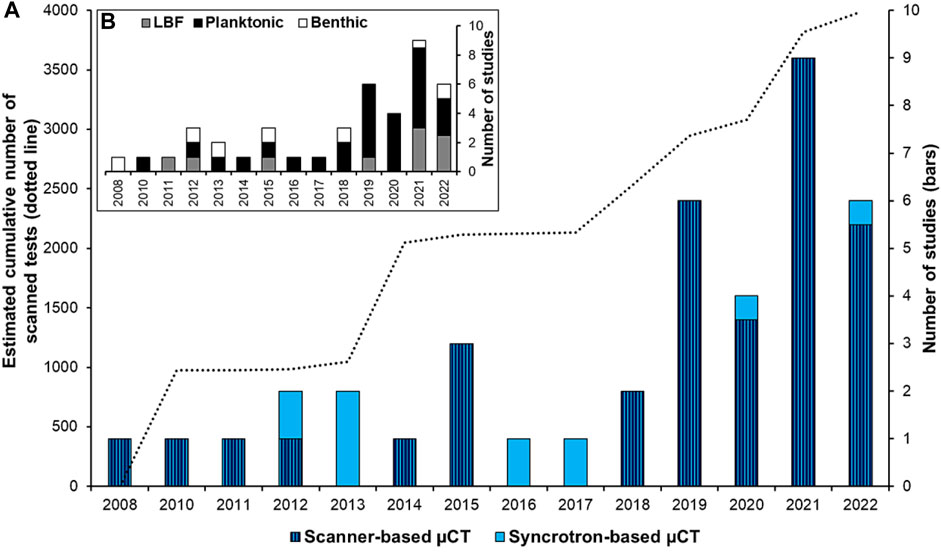
FIGURE 1. (A) Number of studies using 3D foraminifera reconstructions with scanner-based (dark blue with stripes) or synchrotron light-based µCT (light blue), and the estimated number of specimens scanned (dotted line). (B) Number of studies using planktonic (black), large benthic foraminifera (LBF, grey), and benthic foraminifera (white). References are in Supplementary Table S1.

To generate 3D time series based on microfossils, it is necessary to scan as many tests as possible to draw statistically valid conclusions and to work at sub-micrometer resolution for measurement accuracy. One way to reach these objectives is to use a synchrotron light-based approach, a developing method to reveal environmental changes through microfossils records (Foster et al., 2013). The scan time per test is considerably shortened at the synchrotron facility (about 10 min/specimen compared to several hours with a conventional µCT scanner) and the image resolution is generally higher (Supplementary Table S1). However, the synchrotron light-based method has been underused compared to the conventional µCT scanner (Figure 1A). This is probably due to the competitive access to beamtime and the challenge of handling large data sets. In general, morphological parameters such as the thickness and the pore patterns are of great interest for micropaleontological research; the thinning of CaCO₃ tests can be related to a decrease in calcification as a consequence of ocean acidification (e.g., Johnstone et al., 2010; Fox et al., 2020), and pore patterns are increasingly attributed to differences in gas exchange, in particular oxygen uptake, interpreted as a proxy of oxygenation conditions (e.g., Burke et al., 2018; Davis et al., 2021). Extracting these two parameters from 3D tests remains difficult due to the limitations of image processing; therefore, optimizing the post-data analysis is also crucial. Moreover, most previous studies were performed with commercially available software (Supplementary Table S1). Consequently, there is an access limitation for image processing, and a lack of harmonized guidelines, especially when using open-source software adaptable to different microfossil shapes.

We focused our case study on an environmentally vulnerable region, affected by a combination of hydrographic changes and human-induced impacts, the Öresund (the Sound, one part of the Danish Straits), a transition zone between the North Sea, the Skagerrak, and the Baltic Sea (Conley et al., 2007; Charrieau et al., 2018a; Carstensen and Conley, 2019; Carstensen and Duarte, 2019; Charrieau et al., 2019; Ljung et al., 2022). Since the 1940 s, the Baltic Sea has been subjected to multiple stressors such as warming of surface seawater, decreasing pH, expansion of hypoxic areas, and massive increases in burial rates of carbonaceous pollutants from biomass burning (Conley et al., 2007; Rutgersson et al., 2014; Reusch et al., 2018; Carstensen and Duarte, 2019; Ljung et al., 2022). Previously, Charrieau et al. (2019) studied environmental changes in the Öresund region from early industrial (the 1800 s) to present-day conditions (the 2010 s), using a combination of climate modeling, sediment geochemistry, and grain-size distribution together with assemblage studies of benthic foraminifera. In particular, the BFAR (specimens cm⁻² yr⁻¹) of the species Elphidium clavatum (Cushman, 1930) was used to track changes in hydrography. Taking advantage of this historical interesting context and available samples, we extended the analyses on Elphidium clavatum specimens to explore potential changes in their calcite test (i.e., external and internal walls) over time, through synchrotron light-based µCT. Here, we also describe a post-data analysis using open-source software, for quantitatively describing the morphological parameters of the entire test such as average thickness, calcite volume, calcite surface area, number of pores, calcite surface area/volume ratio (calcite SV ratio), and pore density (number of pores/calcite surface area).

We hypothesize that changes in the morphological patterns of foraminiferal tests are generated by environmental variations and should be detectable by 3D reconstructions. We first establish the effects on specimen size and relationships between the different morphological parameters of the entire test. Then, we discuss the interpretations of using morphological variability in 3D time series (i.e., 4D; Tudisco et al., 2019) and morphological traits associated with environmental stressors for palaeoecological interpretations. Finally, we compare the BFAR of Elphidium clavatum (Charrieau et al., 2019) with its morphological changes, to determine whether 3D morphological test variations can be used as an indicator of recent environmental changes and thus complement foraminiferal assemblages.

2 Materials and methods

2.1 Study area and sampling strategy

The Öresund (the Sound) is one of three pathways making up the Danish Straits and a transitional area between the North Sea, through the Kattegat and the Skagerrak, and the Baltic Sea (Figure 2A). The Öresund is a 118 km long narrow strait with an average depth of 23 m and a maximal depth of 53 m at the northeast of the Island of Ven (Figure 2A). The water column is permanently stratified in a two-layer structure; the salty bottom water (salinity ∼29–34; Figure 2B) from the Kattegat penetrates under the brackish layer (salinity ∼8–18; Figure 2B) from the Baltic Sea (Carstensen and Conley, 2019; Charrieau et al., 2019). The stratification is dominated by strong advective transports in both water masses driven by freshwater runoffs, westerly and easterly winds, and the North Atlantic Oscillation (NAO) (Hänninen et al., 2000; Charrieau et al., 2019).

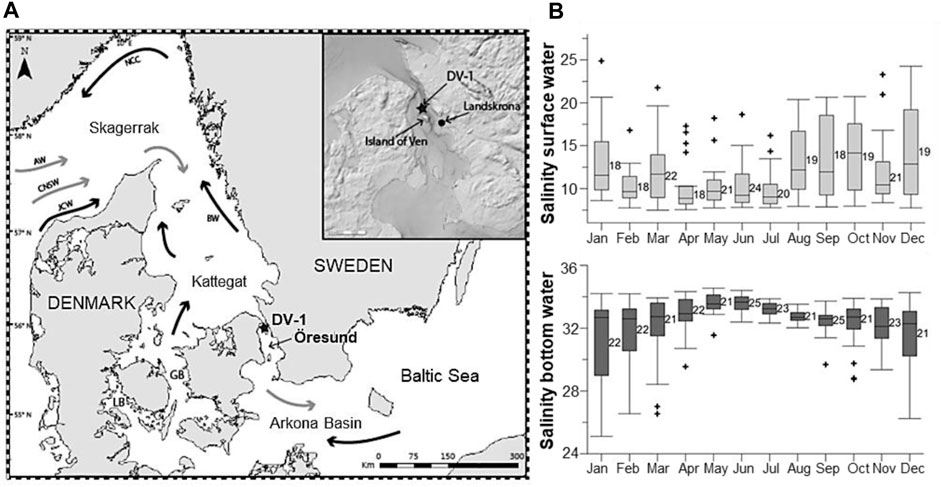
FIGURE 2. (A) Map of the studied area. The star shows the sampling station DV-1 located north of the Island of Ven in the Öresund. GB: Great Belt; LB: Little Belt. General water circulation includes main surface currents (black arrows) and main deep currents (grey arrows). AW: Atlantic Water; CNSW: Central North Sea Water; JCW; Jutland Coastal Water; NCC: Norwegian Coastal Current; BW: Baltic Water. (B) Seasonal variability of salinity (PSU) at the surface water (light grey) and the bottom water (dark grey). The numbers next to the bars indicate the number of measurements for each month between 1965 and 2016. Modified from Charrieau et al. (2019).

Sediment cores were collected in 2013 during a cruise with R/V Skagerak at Öresund station DV-1, to the north of the Island of Ven (55°55.59′ N, 12°42.66′ E; Figure 2A). The sampling details and the age-depth model are described by Charrieau et al. (2019). Briefly, two sediment cores 30 and 36 cm long (named DV1-G and DV1-I, respectively), were sliced into 1-cm layers. The first core (DV1-G) was used to establish the age-depth model, using natural (²¹⁰Pb) and artificial (¹³⁷Cs) radionuclides, while the second core (DV1-I) was used for benthic foraminiferal fauna analysis. The carbon content profiles, measured on both cores, were used to correlate the two cores and establish the age model. The sedimentation rate ranges between 1 and 5.6 mm yr⁻¹ and decreases with depth. Therefore, there is an age uncertainty for the sediment sequence, estimated at ∼1.5 years for the first cm-layers and up to ∼10 years for the deepest layers.

2.2 Benthic foraminifera

In the work of Charrieau et al. (2018a, 2019), foraminiferal specimens from the upper 2 cm of the DV1-I core were wet-picked, while those from the layers below were dry-picked, and sorted under a Nikon stereomicroscope. The benthic foraminiferal assemblage in the Baltic Sea entrance was composed of 76 species; eleven species had a relative abundance higher than 5% and were considered major species (Charrieau et al., 2018a, 2019). The authors of Charrieau et al. (2019) described the flux of foraminifera also known as benthic foraminiferal accumulation rates or BFAR (specimens cm⁻² yr⁻¹) corresponding to the number of specimens per cm³ multiplied by the sediment accumulation rate (cm yr⁻¹). One of the major species of the assemblage indicating large variations in BFAR over the last 200 years is Elphidium clavatum (Charrieau et al., 2019). From the foraminiferal assemblage data, 16 sediment layers were selected, representing the last 200 years (i.e., roughly the years ∼2013, ∼2010, ∼2005, ∼2002, ∼1993, ∼1986, ∼1978, ∼1960, ∼1939, ∼1923, ∼1906, ∼1890, ∼1873, ∼1857, ∼1840, and ∼1807). Between five to ten Elphidium clavatum specimens from the 150–355 µm size fraction (excluding juveniles/smaller specimens; <150 µm) were selected from each layer. The specimens were picked randomly, although visually pristine/unbroken tests were preferentially selected, and a total of 124 specimens were analyzed within the awarded beamtime.

2.3 Stepwise image processing from 3D stacks

The stepwise image processing is summarized in Figure 3 and the details of the procedure are in Supplementary Appendix S1.

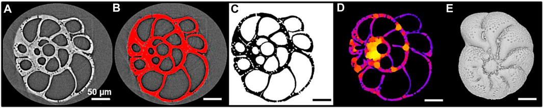
FIGURE 3. Illustration of the stepwise image processing of an Elphidium clavatum specimen (DV4-sp1-2005). (A) Visualization of a stack of raw images in Fiji. (B) Segmentation of the stack in Fiji. (C) Stack of binary images resulting from the segmentation. (D) Local thickness map generated by the BoneJ plugin to calculate automatically the average thickness of the test. (E) 3D reconstruction of the test in MeshLab.

The specimens were scanned at the Beamline BL 47XU, SPring-8 synchrotron facility (Japan). They were mounted on a HiTaCa^®, carbon nanotube (CNT) sheet (Hitachi Zosen Corporation; Fujimoto et al., 2018), to avoid damaging the tests during handling, facilitate test recovery, and enable 3D reconstructions. A voxel size of 0.5 µm with 1800 projections and a 150 m exposure time at 23 keV X-ray energy was used. A stack of raw images was generated for each specimen (Figure 3A) and visualized with the open-source software ImageJ/Fiji (Schindelin et al., 2012). The stack was segmented by dividing the images into fore- and background (test selected in red; Figure 3B) to be converted into a stack of binary images, i.e., the test is in black and the background in white (Figure 3C). This segmentation step is crucial since the accuracy of the measurements depends on the delimitation of the test.

The thickness of the foraminiferal tests is one of the most difficult parameters to measure in its entirety, often limited by cross-section observations and local measurements (Bé and Lott, 1964; Hannah et al., 1994; Weinkauf et al., 2020). Previous studies, using 3D reconstructions, estimated the thickness of the entire test indirectly; from the percentage of calcite volume (i.e., external and internal walls) to total volume (i.e., walls plus chamber cavities) of the test (Titelboim et al., 2021), or the ratio of the calcite volume to calcite surface area (e.g., Zarkogiannis et al., 2020). Here another approach was used, from the stack of binary images, the average thickness of the test was automatically calculated from the local thickness map (Figure 3D) using the BoneJ plugin in Fiji (Dougherty and Kunzelmann, 2007; Doube et al., 2010). This plugin developed for the biomedical field has already been used to explore the average thickness of echinoids (Müter et al., 2015) and pteropod shells (Peck et al., 2018).

In Fiji, the stacks of binary images were converted into “STL” files suitable for 3D reconstructions. Each 3D test was imported into the open-source software MeshLab (Cignoni et al., 2008). Then, the geometric tool was used to measure automatically the volume and surface area of the calcite. Few studies focus on the pore patterns from 3D tests, however, they are analyzed as a 2D image (Burke et al., 2018; Davis et al., 2021). In MeshLab, a topological tool automatically counts the number of “holes” (pores) in the entire test. Therefore, the detected pores are 1) the pores located at the surface connecting the cell and the surrounding environment, and 2) the pores located in the inner walls if they create a detectable hole (e.g., a pore connecting two chambers).

2.4 Adjusted data and statistical analyses

Morphological parameters are generally dependent on the ontogenetic stage (i.e., size-related). All parameters that were significantly correlated with the maximal diameter of the specimens (MDS) (Pearson correlations with Bonferroni correction applied on p-value) were standardized by the average MDS obtained from all specimens. Then, the morphological parameters were adjusted between 0 and one values following the equation:

where $x$ is a morphological value for one specimen, $x\_adjusted$ is the standardized value of $x$ which has values between 0 and 1, $xmin$ is the lowest value on all specimens, and $xmax$ is the highest value on all specimens.

To investigate the relationships between the morphological parameters, Pearson linear correlations, and best-fitted polynomial functions were performed when applicable. The significant level for all the tests was p < 0.05. Non-parametric Mann-Kendall tests were applied to detect significant monotonic trends over the investigated period (Gilbert, 1987). Because of the small sample sizes, non-parametric Kruskal–Wallis tests were conducted to discriminate the specimens between the different years. In case of significant differences, a Dunn post-hoc test with a Bonferoni correction was applied for two-sample comparisons. The statistical tests and boxplots with individual data points were performed using R software (R version 4.2.1, R Core Team).

3 Results

3.1 Exploration of the morphological patterns

The detailed values of the morphological parameters acquired from the 3D tests are available in Supplementary Table S2.

3.1.1 Effects of specimen size

The maximal diameter of the specimens (MDS) and the number of chambers, both related to test size, are weakly positively correlated (Supplementary Figure S1; R² = 0.17, p < 0.0001). Because this study focuses on the entire test measure, the MDS was rather used than the number of chambers. The MDS varies between 149 and 300 µm (Figure 4). The calcite volume (varying from 2.9 E⁺⁰⁵ to 2.8 E⁺⁰⁶ μm³) and the calcite surface area (varying from 1.4 E⁺⁰⁵ to 9.1 E⁺⁰⁵ μm²) increase sharply with the MDS (Figure 4A; R² = 0.76, p < 0.0001, and Figure 4B; R² = 0.65, p < 0.0001, respectively). Well-fitted polynomial functions are also observed between the calcite volume (Figure 4A) and the calcite surface area (Figure 4B) with the MDS. The number of pores is scattered (varying from 356 to 14,559), but increases significantly with the MDS (Figure 4C; R² = 0.16, p < 0.0001). Most of the specimens have <10,000 pores, except four specimens from the early 21st century showing higher values (Figure 4C; Supplementary Table S2). The average thickness indicates scattered values (varying from 2.71 to 11.71 µm), besides a weak but significant increasing correlation with the MDS is observed (Figure 4D; R² = 0.05, p = 0.01).

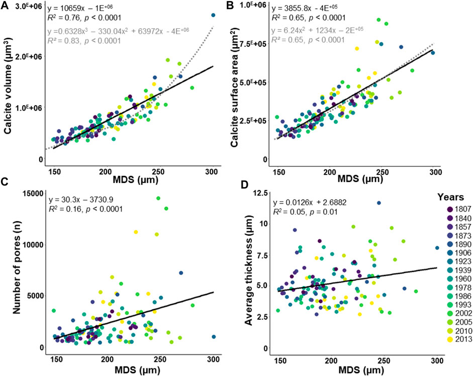
FIGURE 4. Morphological parameters about the maximal diameter of the specimen (MDS). The dataset includes 124 specimens of Elphidium clavatum from the Baltic Sea entrance over the last 200 years (A) Calcite volume (µm³). (B) Calcite surface area (µm²). (C) Number of pores. (D) Average thickness (µm). Linear correlation (black line). Polynomial function (grey dotted line).

3.1.2 Morphological parameters relationships

The calcite volume indicates no significant correlation with the average thickness (Figure 5A; R² = 0.02, p = 0.17). The calcite surface area displays a significant decreasing linear correlation with the average thickness (Figure 5B; R² = 0.36, p < 0.0001). The calcite surface area and calcite volume show a significantly increasing correlation (Figure 5C; R² = 0.21, p < 0.0001). Then, the calcite SV ratio displays a significant decreasing linear correlation with the average thickness (Figure 5D; R² = 0.54, p < 0.0001). Well-fitted polynomial functions are noted between the calcite surface area (Figure 5B; R² = 0.49, p < 0.0001) and the calcite SV ratio (Figure 5D; R² = 0.67, p < 0.0001) with the average thickness. Interestingly, an increasing correlation is found between the average thickness calculated from the BoneJ plugin and the calcite VS ratio used as an indicator of thickness by Zarkogiannis et al. (2020) (Supplementary Figure S2; R² = 0.52, p < 0.0001).

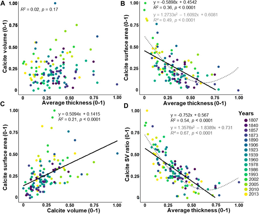
FIGURE 5. Relationships between the average thickness, the calcite volume, and the calcite surface area. The values are adjusted between 0 and 1. The dataset includes 124 specimens of Elphidium clavatum from the Baltic Sea entrance over the last 200 years. (A) Calcite volume and average thickness. (B) Calcite surface area and average thickness. (C) Calcite surface area and calcite volume. (D) Calcite SV ratio and average thickness. Linear correlation (black line). Polynomial function (grey dotted line).

The number of pores in the entire test shows a significantly increasing linear correlation with the calcite surface area (Figure 6A; R² = 0.74, p < 0.0001) and a well-fitted polynomial function (Figure 6A; R² = 0.78, p < 0.0001). The pore density indicates a significant decreasing linear correlation with the average thickness (Figure 6B; R² = 0.48, p < 0.0001) and also a well-fitted polynomial function (Figure 6B; R² = 0.65, p < 0.0001). Weak but significant decreasing correlations are found between the pore density and the calcite volume (Figure 6C; R² = 0.04, p = 0.03, and polynomial function; R² = 0.06, p = 0.03), and a highly significant increasing correlation between the calcite SV ratio and the pore density (Figure 6D; R² = 0.69, p < 0.0001).

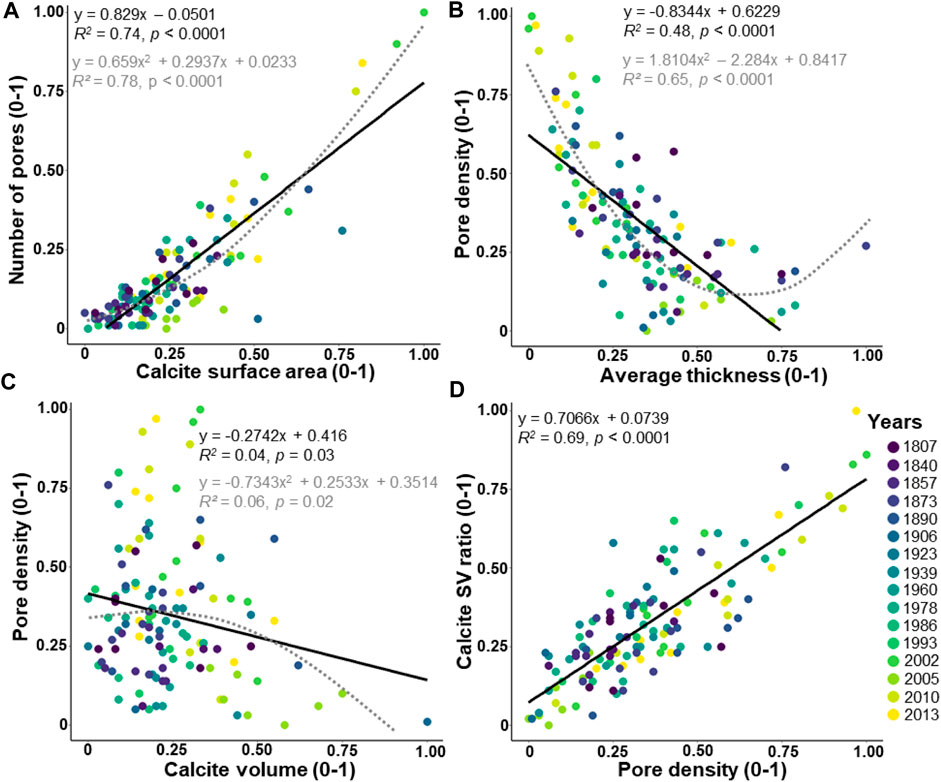
FIGURE 6. Relationships between the pore pattern and the other morphological parameters. The values are adjusted between 0 and 1. The dataset includes 124 specimens of Elphidium clavatum from the Baltic Sea entrance over the last 200 years. (A) Number of pores and calcite surface area. (B) Pore density and average thickness. (C) Pore density and calcite volume. (D) Calcite SV ratio and pore density. Linear correlation (black line). Polynomial function (grey dotted line).

3.2 3D time series

The time series of 3D data, based on the average thickness (Figure 7A), number of pores (Figure 7B), calcite volume (Figure 7C), and calcite surface area (Figure 7D), are not normally distributed (Shapiro normality test, p < 0.0001). The average thickness indicates a significant decreasing trend over the last 200 years (Mann-Kendall: z = 3.26, p = 0.001), whereas the number of pores (Mann-Kendall: z = -2.30, p = 0.02), calcite volume (Mann-Kendall: z = -2.36, p = 0.01), and calcite surface area (Mann-Kendall: z = -3.53, p = 0.0004) indicate significant increasing trends.

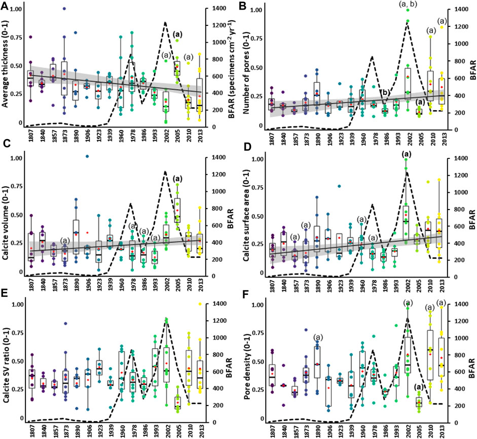
FIGURE 7. 3D time series based on the morphological parameters in Elphidium clavatum from the Baltic Sea entrance over the last 200 years. (A) Average thickness. (B) Number of pores. (C) Calcite volume. (D) Calcite surface area. (E) Calcite SV ratio. (F) Pore density. Boxplots are shown with colored individual data points per estimated year, the red diamond indicates the mean. The morphological values (y-scale) are adjusted (0–1). The bold letters (A, B) indicate significant differences according to Dunn post-hoc test. The dotted line is the BFAR of E. clavatum (specimens cm⁻² yr⁻¹) from Charrieau et al. (2019). A regression line (black line) with a 95% confidence interval (grey area) represents the long-term trend when significant with the Mann-Kendall test.

Significant differences are found between estimated years for the average thickness (Kruskal–Wallis: chi-squared = 32.52, df = 15, p = 0.005), number of pores (Kruskal–Wallis: chi-squared = 40.49, df = 15, p = 0.0003), calcite volume (Kruskal–Wallis: chi-squared = 40.58, df = 15, p = 0.0003), and calcite surface area (Kruskal–Wallis: chi-squared = 43.40, df = 15, p = 0.0001). According to Dunn’s post-hoc test, data for ∼2005 show thicker tests than ∼2002, and ∼2010 (Figure 7A). The number of pores is lower for ∼2005 (Figure 7B) than ∼2013, ∼2010, and ∼2002, then also lower for ∼1986 than ∼2002 (Figure 7B). The calcite volume is larger for ∼2005 than ∼1993, ∼1986, ∼1978, ∼1873, and ∼1807 (Figure 7C). Furthermore, the calcite surface area values are higher for ∼2002 than ∼1986, ∼1978, ∼1873, and ∼1857 (Figure 7D). The statistical values of the posthoc tests are reported in Supplementary Table S3.

The time series of the 3D data for calcite SV ratio (Figure 7E) is non-normally distributed (Shapiro normality test, p = 0.02). The calcite SV ratio time series reveals no significant trend (Mann-Kendall: z = -0.81, p = 0.41). Indeed, most of the boxplots show scattered distributions, such as the years ∼1873, ∼1960, ∼1978, ∼1993, ∼2002, ∼2010, and ∼2013, conversely to condensed distributions observed especially for ∼1986 and ∼2005. Moreover, no significant difference between specimens among years is found (Kruskal–Wallis: chi-squared = 24.98, df = 15, p > 0.05).

The 3D time series of the pore density (Figure 7F) is normally distributed (Shapiro normality test, p = 0.07, and Levene homogeneity of variance test, p = 0.06), but due to the small sample sizes, non-parametric tests are used. The pore density time series indicates no significant trend (Mann-Kendall: z = -1.86, p = 0.06). Except for the years ∼1857, ∼1923, ∼1986, and ∼2005, all the boxplots indicate values with scattered distributions. However, significant differences between years are found (Kruskal–Wallis: chi-squared = 42.71, df = 15, p = 0.0001). According to Dunn’s post-hoc test, the pore density is lower for ∼2005 than ∼1890, ∼2002, ∼2010, and ∼2013.

4 Discussion

The acquisition of morphological parameters such as the average thickness and the number of pores of the entire test was successful, allowing us to reveal the variability of morphological patterns in Elphidium clavatum, as well as long-term trends in a past record. Thus, 3D (i.e., 4D) time series are a promising complement for reconstructing environmental changes in the Baltic Sea entrance over the last 200 years. Based on known morphological patterns in foraminifera associated with environmental stressors e.g., ocean acidification, deoxygenation, and warming, we could infer environmental changes occurring in the region. Furthermore, we expanded the environmental interpretations based on the BFAR changes (Charrieau et al., 2019) and morphological variations in Elphidium clavatum.

4.1 Managing morphological variability in 3D time series

A large variation in morphological patterns could be the result of mixing two pseudocryptic species with slightly different morphologies. Particularly, Elphidium clavatum and Elphidium selseyense (Heron-Allen and Earland, 1911) are morphospecies (Darling et al., 2016), often difficult to distinguish visually, which is why some previous studies grouped E. clavatum and E. selseyense to an E. clavatum-selseyensis complex (Groeneveld et al., 2018; Charrieau et al., 2019; Ni et al., 2020). Morphological variations in foraminifera can be explained by external factors such as adaptation to environmental parameters (i.e., phenotypic adaptation) and/or by internal factors such as adaptation of the genome (heritable trait). There is no evidence of high heritability of thickness and pores but they vary in controlled environmental conditions and across environmental gradients (Burke et al. (2018) and references therein). In this study, we assume that the morphological variations observed from the scanned specimens are related to environmental conditions.

Morphological patterns in Elphidium clavatum fluctuate broadly over the last 200 years (Figure 7). This variability in test morphology may be explained by the seasonal environmental gradients that occurred in the region in terms of salinity (Figure 2B), pH, temperature, and dissolved oxygen concentrations (Charrieau et al., 2019). Moreover, the increase in human activities since the ∼1940 s accentuated the variability range of these environmental conditions, such as the expansion and severity of hypoxic zones (Conley et al., 2007; Reusch et al., 2018; Carstensen and Conley, 2019). As the growth rate of benthic foraminifera can be considered rapid (few months), and their morphology reflects the environment they grew in, here, we consider that the test of adult specimens records approximately up to the seasonal resolution of environmental variations. A significant effort has been achieved in this study to analyze as many specimens as possible at a relatively high temporal resolution, however, the representativeness of the scanned specimens may remain limited to capture the full extent of environmental change.

We argue that large variability in morphological patterns (i.e., scattered distribution) indicates that the Elphidium clavatum specimens calcified in highly contrasted environmental conditions. Furthermore, Weinkauf et al. (2014) reported that an increase in the morphological variability of foraminiferal tests in geological records may be associated with disruptive selection through a stress response. This stress response may lead to increased diversification of the morphology to a maximized chance of some specimens surviving in unfavorable environments (Weinkauf et al., 2014). Conversely, low variability in morphological patterns (i.e., condensed distribution) should reflect that specimens calcified in less contrasted environmental conditions. Indeed, a decrease in morphological variability of shell traits may be attributed to stabilizing selection often associated with reduced environmental fluctuations, and can also be the result of a gradually changing environment (Weinkauf et al., 2014).

4.2 Specimen size and environmental effects on the morphology of entire tests

4.2.1 Effects of specimen size on thickness and pores

Even if the adult specimens come from the same size fraction, the MDS affects the morphology of the entire test but not to the same extent (Figure 4). The calcite volume (Figure 4A) and calcite surface area (Figure 4B) are highly correlated with the size of the specimens, which was already demonstrated in previous studies (Belanger, 2022 and references therein). Because the average thickness is weakly affected by the MDS (Figure 4D), this parameter could be mainly influenced by environmental factors such as varying salinity, pH, or temperature. Conversely, a non-negligible correlation between the number of pores and the MDS was demonstrated (Figure 4C). Comparisons with previous studies are difficult since the pore pattern is species-specific and has only been performed on small parts of the tests from 2D images (Petersen et al., 2016 and references therein). Interestingly, four specimens from the early 21st century may be considered outliers regarding their very high number of pores (Figure 4C). Several hypotheses may explain these outliers; 1) a threshold value (14,559 pores, Supplementary Table S2) because the number of pores can be limited by the robustness of the test and the metabolic demands of the cell (Richirt et al., 2019), 2) an over-estimated number of pores linked to traces of dissolution in some damaged specimens that may generate additional holes, and 3) taphonomic effects that may increase test porosity (Oakes et al., 2019). This contribution illustrates that 3D reconstructions allow quantifying the morphological parameters of tests that have calcified under different environmental conditions, and highlights the need to standardize specimens by the same MDS for more accurate comparisons.

4.2.2 Morphological traits based on environmental stressors

A wide range of morphological patterns in Elphidium clavatum was observed with two distinct patterns; thinner tests have a higher calcite SV ratio (Figure 5D) i.e., a larger surface area (Figure 5B), and a higher pore density (Figure 6B). Conversely, thicker tests have a lower calcite SV ratio and a lower pore density. The well-fitted polynomial functions found between the average thickness and surface calcite area (Figure 5B), calcite SV ratio (Figure 5D), and pore density (Figure 6B), may suggest a compromise between the robustness of the test and the metabolic needs of the cell. This hypothesis can be compared to the scaling laws driving pore patterns described by Richirt et al. (2019). Here, the thickness of the test can have a major role in the pore pattern and the overall shape of the test.

Under natural conditions, it is difficult to associate the variation of morphological patterns with a single environmental factor. However, some morphological traits of foraminifera such as the thickness, SV ratio, and pore density, were previously associated with environmental stressors, allowing us to extrapolate some broad conclusions to Elphidium clavatum for palaeoecological interpretations. We expect that E. clavatum would decrease calcification (i.e., thickness loss) in response to ocean acidification (OA). Indeed, thinner parts of small benthic foraminiferal tests are commonly observed in culture experiments at lower pH values (Allison et al., 2010; Dissard et al., 2010; Haynert et al., 2011). Moreover, the thinning of the entire test (i.e., outer and inner walls) related to OA is also demonstrated in 3D imaging foraminiferal studies (Supplementary Table S1). Ocean acidification is not the only factor that can lead to test thinning. The combined impact of OA and lower salinity may induce a synergistic effect on the calcification process, decreasing resistance to dissolution (Charrieau et al., 2018a; 2018b). Moreover, thinner walls intensify gas exchange in low-oxygen environments (Bernhard, 1986; Sen Gupta and Machain-Castillo, 1993; Kaiho, 1994). The combined effects of warming and OA may have an antagonist effect on calcification due to the positive effect of increasing temperature on calcification and growth (Haynert and Schönfeld, 2014). Consequently, warmer temperatures may also increase the variability in test thickness.

The assumption would be that E. clavatum would have more flattened tests, i.e., a higher calcite SV ratio, in response to deoxygenation and pollution. Some benthic foraminiferal species adapt their tests with flattened shapes to maximize more surface area per unit volume in low-oxygen environments (Bernhard, 1986; Sen Gupta and Machain-Castillo, 1993; Kaiho, 1994). A higher SV ratio can be also associated with a decreasing roundness or an increasing test asymmetry, previously interpreted as an adaptive response toward environmental stress or more variable environmental conditions (Leung et al., 2000; Weinkauf et al., 2014). A decrease in roundness may be also associated with morphological abnormalities. Deformed tests are reported in areas subject to different types of pollution e.g., heavy metals (Alve, 1991), and hydrocarbons (Morvan et al., 2004) but also from areas with a large gradient of salinity such as brackish conditions (Charrieau et al., 2018b). However, lower SV ratios are also observed in benthic foraminifera from high-latitude regions due to the increased volume and size of specimens, probably related to the availability of organic matter even in low-oxygen environments (Belanger, 2022). Therefore, food availability may also increase the calcite SV ratio variability because of a larger calcite volume.

Elphidium clavatum would increase its pore density in response to deoxygenation. In previous studies, correlations are observed between the increase in pore density with lower dissolved oxygen concentrations in the surrounding water (Kuhnt et al., 2013, 2014). Some studies describe that a flattened and thin test facilitates gas exchange by diffusion through the pores by minimizing oxygen consumption and increasing oxygen uptake efficiency (Bradshaw, 1961; Corliss, 1985; Sen Gupta and Machain-Castillo, 1993; Glock et al., 2019). In some benthic foraminifera species from oxygen minimum zones, positive relationships between pore density and temperature, and between pore density and bottom water [NO₃⁻] are demonstrated (Glock et al., 2011; Kuhnt et al., 2013). However, these relationships are species-specific and require further investigation in Elphidium clavatum. In this study, the thinnest tests have a higher pore density (Figure 6B), thus OA may have a synergistic effect with low-oxygen conditions on the pore density. Some authors argue that deoxygenation could lead to higher porosity, i.e., the percentage of the test surface covered by pores (Richirt et al., 2019). Achieving test porosity with 3D imaging remains a challenge, in this contribution, the pore area is visually highly variable between specimens and cannot be studied without robust statistical methods taking into account the variability in test thickness.

4.3 3D time series to reconstruct recent environmental changes in the Baltic Sea entrance

4.3.1 Long-term trends in morphological changes

Although the morphological variability is large, significant long-term trends in morphological changes over the last 200 years can be noted, especially in the average thickness, number of pores, calcite volume, and calcite surface area (Figure 7). We computed the decrease in average thickness, and the increase in the number of pores, calcite volume, and surface area from the modern foraminifera in ∼2013 compared to their historical counterparts in ∼1807 (details in Supplementary Table S4). The modern specimens reveal a thickness loss of 28 ± 14% (n = 18), an increase of 35 ± 11% in calcite surface area, an increase of 15 ± 4% in calcite volume, and an increase of 91 ± 67% in the number of pores. These long-term trends can be interpreted as the result of gradual environmental changes in the Baltic Sea entrance. Fox et al. (2020) demonstrate a larger reduction in shell thickness of up to 76% in the planktonic foraminifera Neogloboquadrina dutertrei over the last ∼140 years in the Pacific ocean. These authors also find a thickness loss of ∼20% in Globigerinoides ruber (Fox et al., 2020), corresponding to a similar result for Elphidium clavatum. Globigerinoides ruber is known to display a mechanism of resistance to OA linked to photosynthetic algal symbionts (Fox et al., 2020 and references therein). The same mechanism of resistance for Elphidium clavatum cannot be applied, as they are living in the aphotic zone. Putative mechanisms of resistance to OA in non-photosynthetically benthic foraminifera from high-latitude regions need to be further investigated.

4.3.2 Comparisons of environmental interpretations based on BFAR and morphology in Elphidium clavatum

During the early industrial period referring to the period from ∼1807 to 1939 in our historical context, the BFAR of Elphidium clavatum remained stable and low (<44 specimens cm⁻² yr⁻¹) (Figure 7, Charrieau et al., 2019). From the total foraminiferal assemblage in Charrieau et al. (2019), two subzones were described ∼1807–1873 and ∼1873–1923, with associated environmental conditions characterized by low oxygen conditions, a salinity of ∼30, and the onset of human-induced impacts with various types of pollution (Zillén et al., 2008; Charrieau et al., 2019; Ljung et al., 2022). No significant difference was found in the morphology of the Elphidium clavatum specimens between the two subzones, however, the variations in both BFAR and the morphological parameters are not synchronized. Although the BFAR remained unchanged, a large variability in test thickness, calcite SV ratio, and pore density can be observed in ∼1873. The relative stability of the morphological patterns excepted in ∼1873 indicates a pivotal period, already noted by Charrieau et al. (2019), suggesting wider variability in pH and [O₂] values. In summary, during the early industrial period, although the BFAR of Elphidium clavatum remained unchanged, the morphological variations instead reveal the natural variability of environmental conditions in the region.

The ∼1939–2002 period corresponds to the intensification of human activities in the region, such as the massive increase of carbonaceous pollution from petroleum products for energy use (Ljung et al., 2022), and excess nutrient loading from terrestrial to marine environments (Gustafsson et al., 2012). This period was marked by favorable growth conditions of Elphidium clavatum with two successive sharp increases in the BFAR up to 826 and 1,247 specimens cm⁻² yr⁻¹ in ∼1939–1978 and ∼1986–2002 respectively (Charrieau et al., 2019). These BFAR variations were previously associated with the increase in organic matter as a food source for foraminifera, and major changes in the current and sediment pattern (Charrieau et al., 2019 and references therein). Interestingly, there is a synchronicity between both increases in BFAR and morphological variability, especially for the average thickness, calcite SV ratio, and pore density. Further, the decrease in the BFAR from the short period ∼1978–1986 (276 specimens cm⁻² yr⁻¹) was associated with the improved environmental conditions to reduce eutrophication in the region (Carstensen et al., 2006; Conley et al., 2007; Charrieau et al., 2019). A decrease in variability for all the morphological parameters is observed in ∼1986, suggesting that the specimens calcified in less contrasted environmental conditions. In summary, the historical record of Elphidium clavatum reveals the intensification of anthropogenic activities through the synchrony between high reproductive success and broad morphological diversification and conversely reduced variability in test morphology that may be associated with a short event of improved environmental conditions.

The early 21st century foraminiferal record reveals sharp contrasts between the BFAR and morphological variations in Elphidium clavatum. The associated environmental conditions during this period were characterized by low oxygen conditions, high organic matter content, and open ocean salinity (Charrieau et al., 2019). Particularly in ∼2002, E. clavatum dominated the fauna (Charrieau et al., 2019), but the specimens are the most negatively affected over the last 200 years: the average thickness compared to those from ∼1807 has decreased by 36 ± 17% (n = 18), the calcite surface area has increased by 63 ± 21%, and the number of pores has increased by 151 ± 120% (Supplementary Table S4). Moreover, in ∼2002 the largest variability in the calcite SV ratio and pore density is observed for the whole record (Figure 7). These results can be attributed to the larger seasonal hypoxia event recorded in the Danish Straits in 2002, explained by the combination of bottom water transport, nutrient supply from land, and rising temperature (Conley et al., 2007). By contrast in ∼2005, the morphological variability is lower and the specimens significantly differ from the general patterns observed around the 21st century (Figure 7). Especially, the specimens are thicker 11 ± 6% (n= 15), with a larger calcite volume of 77 ± 15% and a lower number of pores of 54 ± 26% compared to those from the ∼1807 (Supplementary Table S4). These unexpected results may be related to a massive inflow of highly saline, cold, and extremely oxygen-rich water from the North Sea, called Major Baltic Inflows, affecting occasionally the deep basins of the Baltic Sea and reported in 2003 (Lehmann et al., 2004; Feistel et al., 2006). Then, from the 2010s, a desynchronization is notable between the lower and stable BFAR (∼225 specimens cm⁻² yr⁻¹) and the large morphological variations of all parameters (Figure 7). The persisting environmental stressors i.e., warming, hypoxia, and OA since the 1940s, in addition to the possible inter-specific competition with opportunistic species such as Nonionella sp. T1 and Nonionoides turgidus (Charrieau et al., 2019), would not allow Elphidium clavatum to combine high reproductive success with a wide diversification of its morphological patterns. Recently, Bernhard et al. (2021) demonstrated in a triple-stressors experiment with propagules that Elphidium cf E. excavatum indicates high abundance under pre-industrial and cold acidified conditions, low abundance in present-day and cool + OA + hypoxic conditions, and absence in warm + OA + hypoxic conditions, indicating that Elphidium clavatum and probably other species from high-latitude regions will be challenged in the next decades.

5 Conclusion

We analyzed 3D time series from 124 foraminiferal specimens, recording the period from early industrial (the 1800 s) to present-day (the 2010 s) conditions in the Baltic Sea entrance. The BFAR (specimens cm⁻² y⁻¹) changed profoundly in this vulnerable region subject to natural hydrographic changes and increasing anthropogenic pressures (Charrieau et al., 2019). Here, 3D time series (i.e., 4D) of morphological patterns in Elphidium clavatum provide a promising complement to reconstruct the Baltic Sea entrance evaluation over the last 200 years. We demonstrate long-term morphological trends such as the decrease in test average thickness by ∼28% (up to 36% in ∼2002) and the increase in the number of pores by ∼91% (up to 151% in ∼2002), revealing that foraminifera are being negatively affected through a multiple stressors situation such as ocean acidification, deoxygenation, and warming. We interpret that a large morphological variability is associated with highly contrasting environmental conditions, and conversely lower morphological variability results from more stable conditions. Over the last two centuries, the variations in the BFAR and the morphological patterns in E. clavatum are not always synchronous. In the early industrial period, the BFAR remained unchanged while the variability in pore density fluctuates broadly, suggesting periods with large natural variations in bottom-water oxygenation conditions. From the 1940 s corresponding to the intensification of human activities, increases in BFAR and morphological variability are synchronous, revealing more contrasting seasonal environmental conditions. Finally, in the early 21st century, the BFAR was stable while morphological variations remain large, suggesting a persistent multiple stressors situation. Our project highlights the value of using 3D time series of calcifying microfossils from existing geological archives to quantify the effects of anthropogenic climate change and provide additional information to foraminiferal assemblages studies.

Data availability statement

The original contributions presented in the study are included in the article/Supplementary Material, further inquiries can be directed to the corresponding authors.

Author contributions

HF and LC collected the samples. DM, LC, SN, KH, and YS scanned the samples. CC, DM, and BP worked on the 3D image processing. CC performed the statistical analyses. CC and HF wrote the manuscript. All authors provided manuscript comments and approved the final version.

Funding

This work was supported by the Swedish Research Council Formas (grant 2012-2140) and the Swedish Research Council VR (grant 2017-00671), the Royal Physiographic Society, Crafoord and the Oscar and Lili Lamm Foundations, the Interreg project “MAX4ESSFUN Cross Border Network and Researcher Programme”. We thank SPring-8 for beamtime under proposal numbers 2018A1099, 2018B1241, and 2020A1221.

Acknowledgments

We thank the captain and crew of r/v Skagerak, Karl Ljung, and Petra Schoon for assistance during core collection, and the staff at the SPring-8 synchrotron facility (BL 47XU). We in particular thank Kentaro Uesugi, who was very helpful in the process of foraminifera shells scanning at the synchrotron SPring-8 (Japan). We are very grateful to the editor SZ and the three reviewers.

Conflict of interest

Author DM is employed by the company FORCE Technology.

The remaining authors declare that the research was conducted in the absence of any commercial or financial relationships that could be construed as a potential conflict of interest.

Publisher’s note

All claims expressed in this article are solely those of the authors and do not necessarily represent those of their affiliated organizations, or those of the publisher, the editors and the reviewers. Any product that may be evaluated in this article, or claim that may be made by its manufacturer, is not guaranteed or endorsed by the publisher.

Supplementary material

The Supplementary Material for this article can be found online at: https://www.frontiersin.org/articles/10.3389/feart.2023.1120170/full#supplementary-material

References

Allison, N., Austin, W., Paterson, D., and Austin, H. (2010). Culture studies of the benthic foraminifera Elphidium williamsoni: Evaluating pH, ∆[CO32−] and inter-individual effects on test Mg/Ca. Chem. Geol. 274, 87–93. doi:10.1016/j.chemgeo.2010.03.019
Alve, E. (1991). Benthic foraminifera in sediment cores reflecting heavy metal pollution in Sorfjord, Western Norway. J. Foraminifer. Res. 21, 1–19. doi:10.2113/gsjfr.21.1.1
Bé, A. W. H., and Lott, L. (1964). Shell growth and structure of planktonic foraminifera. Science 145, 823–824. doi:10.1126/science.145.3634.823
Belanger, C. L. (2022). Volumetric analysis of benthic foraminifera: Intraspecific test size and growth patterns related to embryonic size and food resources. Mar. Micropaleontol. 176, 102170. doi:10.1016/j.marmicro.2022.102170
Bernhard, J. M. (1986). Characteristic assemblages and morphologies of benthic foraminifera from anoxic, organic-rich deposits; Jurassic through Holocene. J. Foraminifer. Res. 16, 207–215. doi:10.2113/gsjfr.16.3.207
Bernhard, J. M., Wit, J. C., Starczak, V. R., Beaudoin, D. J., Phalen, W. G., and McCorkle, D. C. (2021). Impacts of multiple stressors on a benthic foraminiferal community: A long-term experiment assessing response to ocean acidification, hypoxia and warming. Front. Mar. Sci. 8. doi:10.3389/fmars.2021.643339
Bijma, J., Pörtner, H.-O., Yesson, C., and Rogers, A. D. (2013). Climate change and the oceans – what does the future hold? Mar. Pollut. Bull., the global state of the ocean; interactions between stresses, impacts and some potential solutions. Synthesis Pap. Int. Programme State Ocean 2011 2012 Work. 74, 495–505. doi:10.1016/j.marpolbul.2013.07.022
Bindoff, N. L., Cheung, W. W. L., Kairo, J. G., Arístegui, J., Guinder, V. A., Hallberg, R., et al. (2019). “Changing ocean, marine ecosystems, and dependent communities,” in IPCC special report on the ocean and cryosphere in a changing climate. Editors H.-O. Pörtner, D. C. Roberts, V. Masson-Delmotte, P. Zhai, M. Tignor, E. Poloczanskaet al. (Switzerland: Intergovernmental Panel on Climate Change), 477–587.
Bradshaw, J. S. (1961). Laboratory experiments on the ecology of foraminifera. Cushman Found. Foram Res. Contr 12, 87–106.
Breitburg, D., Levin, L. A., Oschlies, A., Grégoire, M., Chavez, F. P., Conley, D. J., et al. (2018). Declining oxygen in the global ocean and coastal waters. Science 359, eaam7240. doi:10.1126/science.aam7240
Burke, J. E., Renema, W., Henehan, M. J., Elder, L. E., Davis, C. V., Maas, A. E., et al. (2018). Factors influencing test porosity in planktonic foraminifera. Biogeosciences 15, 6607–6619. doi:10.5194/bg-15-6607-2018
Carstensen, J., Conley, D. J., Andersen, J. H., and Ærtebjerg, G. (2006). Coastal eutrophication and trend reversal: A Danish case study. Limnol. Oceanogr. 51, 398–408. doi:10.4319/lo.2006.51.1_part_2.0398
Carstensen, J., and Conley, D. J. (2019). Baltic sea hypoxia takes many shapes and sizes. Limnol. Oceanogr. Bull. 28, 125–129. doi:10.1002/lob.10350
Carstensen, J., and Duarte, C. M. (2019). Drivers of pH variability in coastal ecosystems. Environ. Sci. Technol. 53, 4020–4029. doi:10.1021/acs.est.8b03655
Charrieau, L. M., Filipsson, H. L., Ljung, K., Chierici, M., Knudsen, K. L., and Kritzberg, E. (2018a). The effects of multiple stressors on the distribution of coastal benthic foraminifera: A case study from the skagerrak-baltic sea region. Mar. Micropaleontol. 139, 42–56. doi:10.1016/j.marmicro.2017.11.004
Charrieau, L. M., Filipsson, H. L., Nagai, Y., Kawada, S., Ljung, K., Kritzberg, E., et al. (2018b). Decalcification and survival of benthic foraminifera under the combined impacts of varying pH and salinity. Mar. Environ. Res. 138, 36–45. doi:10.1016/j.marenvres.2018.03.015
Charrieau, L. M., Ljung, K., Schenk, F., Daewel, U., Kritzberg, E., and Filipsson, H. L. (2019). Rapid environmental responses to climate-induced hydrographic changes in the Baltic Sea entrance. Biogeosciences 16, 3835–3852. doi:10.5194/bg-16-3835-2019
Cignoni, P., Callieri, M., Corsini, M., Dellepiane, M., Ganovelli, F., and Ranzuglia, G. (2008). MeshLab: An open-source mesh processing tool 8.
Conley, D. J., Carstensen, J., Ærtebjerg, G., Christensen, P. B., Dalsgaard, T., Hansen, J. L. S., et al. (2007). Long-term changes and impacts of hypoxia in Danish coastal waters. Ecol. Appl. 17, S165–S184. doi:10.1890/05-0766.1
Corliss, B. H. (1985). Microhabitats of benthic foraminifera within deep-sea sediments. Nature 314, 435–438. doi:10.1038/314435a0
Cushman, J. A. (1930). The foraminifera of the atlantic ocean, part 7 – nonionidae, camerinidae, peneroplidae and alveonellidae. Bull. U. S. Natl. Mus. 104, 1–79.
Darling, K. F., Schweizer, M., Knudsen, K. L., Evans, K. M., Bird, C., Roberts, A., et al. (2016). The genetic diversity, phylogeography and morphology of Elphidiidae (Foraminifera) in the Northeast Atlantic. Mar. Micropaleontol. 129, 1–23. doi:10.1016/j.marmicro.2016.09.001
Davis, C. V., Wishner, K., Renema, W., and Hull, P. M. (2021). Vertical distribution of planktic foraminifera through an oxygen minimum zone: How assemblages and test morphology reflect oxygen concentrations. Biogeosciences 18, 977–992. doi:10.5194/bg-18-977-2021
Dissard, D., Nehrke, G., Reichart, G. J., and Bijma, J. (2010). Impact of seawater pCO2 on calcification and Mg/Ca and Sr/Ca ratios in benthic foraminifera calcite: Results from culturing experiments with Ammonia tepida. Biogeosciences 7, 81–93. doi:10.5194/bg-7-81-2010
Doube, M., Kłosowski, M. M., Arganda-Carreras, I., Cordelières, F. P., Dougherty, R. P., Jackson, J. S., et al. (2010). BoneJ: Free and extensible bone image analysis in ImageJ. Bone 47, 1076–1079. doi:10.1016/j.bone.2010.08.023
Dougherty, R., and Kunzelmann, K.-H. (2007). Computing local thickness of 3D structures with ImageJ. Microsc. Microanal. 13, 1678–1679. doi:10.1017/S1431927607074430
Feistel, R., Nausch, G., and Hagen, E. (2006). Unusual Baltic inflow activity in 2002-2003 and varying deep-water properties. Oceanologia 48, 21–35.
Foster, L. C., Schmidt, D. N., Thomas, E., Arndt, S., and Ridgwell, A. (2013). Surviving rapid climate change in the deep sea during the Paleogene hyperthermals. Proc. Natl. Acad. Sci. 110, 9273–9276. doi:10.1073/pnas.1300579110
Fox, L., Stukins, S., Hill, T., and Miller, C. G. (2020). Quantifying the effect of anthropogenic climate change on calcifying plankton. Sci. Rep. 10, 1620. doi:10.1038/s41598-020-58501-w
Fujimoto, N., Maruyama, H., Kawakami, Y., and Yamashita, T. (2018). Development of applications for aligned carbon nanotubes (HiTaCa). Hitz 79, 59–63.
Gilbert, R. O. (1987). Statistical methods for environmental pollution monitoring. New York: van Nostrand Reinhold.
Glock, N., Eisenhauer, A., Milker, Y., Liebetrau, V., Schönfeld, J., Mallon, J., et al. (2011). Environmental influences on the pore density of Bolivina spissa (Cushman). J. Foraminifer. Res. 41, 22–32. doi:10.2113/gsjfr.41.1.22
Glock, N., Roy, A.-S., Romero, D., Wein, T., Weissenbach, J., Revsbech, N. P., et al. (2019). Metabolic preference of nitrate over oxygen as an electron acceptor in foraminifera from the Peruvian oxygen minimum zone. Proc. Natl. Acad. Sci. 116, 2860–2865. doi:10.1073/pnas.1813887116
Groeneveld, J., Filipsson, H. L., Austin, W. E. N., Darling, K., McCarthy, D., Quintana Krupinski, N. B., et al. (2018). Assessing proxy signatures of temperature, salinity, and hypoxia in the Baltic Sea through foraminifera-based geochemistry and faunal assemblages. J. Micropalaeontology 37, 403–429. doi:10.5194/jm-37-403-2018
Gruber, N. (2011). Warming up, turning sour, losing breath: Ocean biogeochemistry under global change. Philos. Trans. R. Soc. Math. Phys. Eng. Sci. 369, 1980–1996. doi:10.1098/rsta.2011.0003
Gustafsson, B. G., Schenk, F., Blenckner, T., Eilola, K., Meier, H. E. M., Müller-Karulis, B., et al. (2012). Reconstructing the development of Baltic Sea eutrophication 1850–2006. AMBIO 41, 534–548. doi:10.1007/s13280-012-0318-x
Hannah, F., Rogerson, R., and Laybourn-Parry, J. (1994). Respiration rates and biovolumes of common benthic Foraminifera (Protozoa). J. Mar. Biol. Assoc. U. K. 74, 301–312. doi:10.1017/S0025315400039345
Hänninen, J., Vuorinen, I., and Hjelt, P. (2000). Climatic factors in the Atlantic control the oceanographic and ecological changes in the Baltic Sea. Limnol. Oceanogr. 45, 703–710. doi:10.4319/lo.2000.45.3.0703
Haynert, K., and Schönfeld, J. (2014). Impact of changing carbonate chemistry, temperature, and salinity on growth and test degradation of the benthic foraminifer. Ammon. aomoriensis J. Foraminifer. Res. 44, 76–89. doi:10.2113/gsjfr.44.2.76
Haynert, K., Schönfeld, J., Riebesell, U., and Polovodova, I. (2011). Biometry and dissolution features of the benthic foraminifer Ammonia aomoriensis at high pCO₂. Mar. Ecol. Prog. Ser. 432, 53–67. doi:10.3354/meps09138
Heron-Allen, E., and Earland, A. (1911). On recent and fossil foraminifera of the shore sands at Selsey Bill, Sussex. J. R. Microsc. Soc. Lond. Part. 8, 436–448.
Howes, E. L., Eagle, R. A., Gattuso, J.-P., and Bijma, J. (2017). Comparison of Mediterranean pteropod shell biometrics and ultrastructure from historical (1910 and 1921) and present day (2012) samples provides baseline for monitoring effects of global change. PLOS ONE 12, e0167891. doi:10.1371/journal.pone.0167891
Johnstone, H. J. H., Schulz, M., Barker, S., and Elderfield, H. (2010). Inside story: An X-ray computed tomography method for assessing dissolution in the tests of planktonic foraminifera. Mar. Micropaleontol. 77, 58–70. doi:10.1016/j.marmicro.2010.07.004
Kaiho, K. (1994). Benthic foraminiferal dissolved-oxygen index and dissolved-oxygen levels in the modern ocean. Geology 22, 719–722. doi:10.1130/0091-7613(1994)022<0719:BFDOIA>2.3.CO;2
Kroeker, K. J., Kordas, R. L., Crim, R., Hendriks, I. E., Ramajo, L., Singh, G. S., et al. (2013). Impacts of ocean acidification on marine organisms: Quantifying sensitivities and interaction with warming. Glob. Change Biol. 19, 1884–1896. doi:10.1111/gcb.12179
Kuhnt, T., Friedrich, O., Schmiedl, G., Milker, Y., Mackensen, A., and Lückge, A. (2013). Relationship between pore density in benthic foraminifera and bottom-water oxygen content. Deep Sea Res. Part Oceanogr. Res. Pap. 76, 85–95. doi:10.1016/j.dsr.2012.11.013
Kuhnt, T., Schiebel, R., Schmiedl, G., Milker, Y., Mackensen, A., and Friedrich, O. (2014). Automated and manuel analyses of the pore density-to-oxygen relationship in Globobulimina turgida (Bailey). J. Foraminifer. Res. 44, 5–16. doi:10.2113/gsjfr.44.1.5
Lehmann, A., Lorenz, P., and Jacob, D. (2004). Modelling the exceptional Baltic Sea inflow events in 2002–2003. Geophys. Res. Lett. 31. doi:10.1029/2004GL020830
Leung, B., Forbes, M. R., and Houle, D. (2000). Fluctuating asymmetry as a bioindicator of stress: Comparing efficacy of analyses involving multiple traits. Am. Nat. 155, 101–115. doi:10.1086/303298
Liew, T.-S., and Schilthuizen, M. (2016). A method for quantifying, visualising, and analysing gastropod shell form. PLOS ONE 11, e0157069. doi:10.1371/journal.pone.0157069
Ljung, K., Schoon, P. L., Rudolf, M., Charrieau, L. M., Ni, S., and Filipsson, H. L. (2022). Recent increased loading of carbonaceous pollution from biomass burning in the baltic sea. ACS Omega 7, 35102–35108. doi:10.1021/acsomega.2c04009
Meredith, M., Sommerkorn, M., Cassota, S., Derksen, C., Ekaykin, A., Hollowed, A., et al. (2019). Polar Regions. Chapter 3, IPCC special report on the ocean and cryosphere in a changing climate. Available at: https://www.ipcc.ch/srocc/chapter/chapter-3-2/.
Monnet, C., Zollikofer, C., Bucher, H., and Goudemand, N. (2009). Three-dimensional morphometric ontogeny of mollusc shells by micro-computed tomography and geometric analysis. Palaeontol. Electron. 12, 1–13. doi:10.5167/uzh-23587
Morvan, J., Cadre, V. L., Jorissen, F., and Debenay, J.-P. (2004). Foraminifera as potential bio-indicators of the “Erika” oil spill in the Bay of Bourgneuf: Field and experimental studies. Aquat. Living Resour. 17, 317–322. doi:10.1051/alr:2004034
Müter, D., Sørensen, H. O., Oddershede, J., Dalby, K. N., and Stipp, S. L. S. (2015). Microstructure and micromechanics of the heart urchin test from X-ray tomography. Acta Biomater. 23, 21–26. doi:10.1016/j.actbio.2015.05.007
Ni, S., Quintana Krupinski, N. B., Groeneveld, J., Persson, P., Somogyi, A., Brinkmann, I., et al. (2020). Early diagenesis of foraminiferal calcite under anoxic conditions: A case study from the landsort deep, Baltic Sea (iodp site M0063). Chem. Geol. 558, 119871. doi:10.1016/j.chemgeo.2020.119871
Oakes, R. L., Peck, V. L., Manno, C., and Bralower, T. J. (2019). Degradation of internal organic matter is the main control on pteropod shell dissolution after death. Glob. Biogeochem. Cycles 33, 749–760. doi:10.1029/2019GB006223
Peck, V. L., Oakes, R. L., Harper, E. M., Manno, C., and Tarling, G. A. (2018). Pteropods counter mechanical damage and dissolution through extensive shell repair. Nat. Commun. 9, 264. doi:10.1038/s41467-017-02692-w
Petersen, J., Riedel, B., Barras, C., Pays, O., Guihéneuf, A., Mabilleau, G., et al. (2016). Improved methodology for measuring pore patterns in the benthic foraminiferal genus Ammonia. Mar. Micropaleontol. 128, 1–13. doi:10.1016/j.marmicro.2016.08.001
Reusch, T. B. H., Dierking, J., Andersson, H. C., Bonsdorff, E., Carstensen, J., Casini, M., et al. (2018). The Baltic Sea as a time machine for the future coastal ocean. Sci. Adv. 4, eaar8195. doi:10.1126/sciadv.aar8195
Rhein, M., Rintoul, S. R., Aoki, S., Campos, E., Chambers, D., Feely, R. A., et al. (2013). “Observations: Ocean,” in Climate change 2013: The physical science basis. Contribution of working group I to the fifth assessment report of the intergovernmental panel on climate change.
Richirt, J., Champmartin, S., Schweizer, M., Mouret, A., Petersen, J., Ambari, A., et al. (2019). Scaling laws explain foraminiferal pore patterns. Sci. Rep. 9, 9149. doi:10.1038/s41598-019-45617-x
Rutgersson, A., Jaagus, J., Schenk, F., and Stendel, M. (2014). Observed changes and variability of atmospheric parameters in the Baltic Sea region during the last 200 years. Clim. Res. 61, 177–190. doi:10.3354/cr01244
Schindelin, J., Arganda-Carreras, I., Frise, E., Kaynig, V., Longair, M., Pietzsch, T., et al. (2012). Fiji: An open-source platform for biological-image analysis. Nat. Methods 9, 676–682. doi:10.1038/nmeth.2019
Sen Gupta, B. K., and Machain-Castillo, M. L. (1993). Benthic foraminifera in oxygen-poor habitats. Mar. Micropaleontol. 20, 183–201. doi:10.1016/0377-8398(93)90032-S
Speijer, R. P., Loo, D. V., Masschaele, B., Vlassenbroeck, J., Cnudde, V., and Jacobs, P. (2008). Quantifying foraminiferal growth with high-resolution X-ray computed tomography: New opportunities in foraminiferal ontogeny, phylogeny, and paleoceanographic applications. Geosphere 4, 760–763. doi:10.1130/GES00176.1
Steffen, W., Broadgate, W., Deutsch, L., Gaffney, O., and Ludwig, C. (2015). The trajectory of the anthropocene: The great acceleration. Anthr. Rev. 2, 81–98. doi:10.1177/2053019614564785
Strong, A. L., Kroeker, K. J., Teneva, L. T., Mease, L. A., and Kelly, R. P. (2014). ocean acidification 2.0: Managing our changing coastal ocean chemistry. BioScience 64, 581–592. doi:10.1093/biosci/biu072
Titelboim, D., Lord, O. T., and Schmidt, D. N. (2021). Thermal stress reduces carbonate production of benthic foraminifera and changes the material properties of their shells. ICES J. Mar. Sci. 78, 3202–3211. doi:10.1093/icesjms/fsab186
Tudisco, E., Etxegarai, M., Hall, S. A., Charalampidou, E.-M., Couples, G. D., Lewis, H., et al. (2019). Fast 4-D imaging of fluid flow in rock by high-speed neutron tomography. J. Geophys. Res. Solid Earth 124, 3557–3569. doi:10.1029/2018JB016522
Weinkauf, M. F. G., Moller, T., Koch, M. C., and Kučera, M. (2014). Disruptive selection and bet-hedging in planktonic foraminifera: Shell morphology as predictor of extinctions. Front. Ecol. Evol. 2. doi:10.3389/fevo.2014.00064
Weinkauf, M. F. G., Zwick, M. M., and Kučera, M. (2020). Constraining the role of shell porosity in the regulation of shell calcification intensity in the modern planktonic foraminifer Orbulina Universa d’Orbigny. J. Foraminifer. Res. 50, 195–203. doi:10.2113/gsjfr.50.2.195
Zarkogiannis, S. D., Fernandez, V., Greaves, M., Mortyn, P. G., Kontakiotis, G., Antonarakou, A., et al. (2020). X-ray tomographic data of planktonic foraminifera species Globigerina bulloides from the Eastern Tropical Atlantic across Termination II. Gigabyte 2020, 1–10. doi:10.46471/gigabyte.5
Keywords: foraminifera, tomography, 3D reconstructions, synchrotron-light, environmental change, morphological variability
Citation: Choquel C, Müter D, Ni S, Pirzamanbein B, Charrieau LM, Hirose K, Seto Y, Schmiedl G and Filipsson HL (2023) 3D morphological variability in foraminifera unravel environmental changes in the Baltic Sea entrance over the last 200 years. Front. Earth Sci. 11:1120170. doi: 10.3389/feart.2023.1120170
Received: 09 December 2022; Accepted: 15 March 2023;
Published: 03 April 2023.
Edited by:
Stergios D. Zarkogiannis, University of Oxford, United KingdomReviewed by:
Danna Titelboim, University of Oxford, United KingdomShunichi Kinoshita, National Museum of Nature and Science, Japan
Ashley Burkett, Oklahoma State University, United States
Copyright © 2023 Choquel, Müter, Ni, Pirzamanbein, Charrieau, Hirose, Seto, Schmiedl and Filipsson. This is an open-access article distributed under the terms of the Creative Commons Attribution License (CC BY). The use, distribution or reproduction in other forums is permitted, provided the original author(s) and the copyright owner(s) are credited and that the original publication in this journal is cited, in accordance with accepted academic practice. No use, distribution or reproduction is permitted which does not comply with these terms.
*Correspondence: Constance Choquel, constance.choquel@geol.lu.se; Helena L. Filipsson, helena.filipsson@geol.lu.se