Influence of the matrix of the soil-rock mixture on deformation and failure behaviors of the slope based on material point method

Li, Xia; Tang, Shanyanqin; Zheng, Yong; Liu, Jie; Wang, Liejian; He, Kaiyuan; Jiang, Tao

doi:10.3389/feart.2022.997928

ORIGINAL RESEARCH article

Front. Earth Sci., 13 September 2022
Sec. Geohazards and Georisks
Volume 10 - 2022 | https://doi.org/10.3389/feart.2022.997928

Influence of the matrix of the soil-rock mixture on deformation and failure behaviors of the slope based on material point method

Xia Li¹

Shanyanqin Tang¹

Yong Zheng^1,2* www.frontiersin.org

Jie Liu³

Liejian Wang³ www.frontiersin.org

Kaiyuan He¹ www.frontiersin.org

Tao Jiang⁴

¹School of River and Ocean Engineering, Chongqing Jiaotong University, Chongqing, China
²Key Laboratory of Geological Hazards Mitigation for Mountainous Highway and Waterway, Chongqing Municipal Education Commission, Chongqing, China
³Chongqing Water Conservancy and Electric Power Survey and Design Institute Co., Ltd, Chongqing, China
⁴State Key Laboratory of Geohazard Prevention and Geoenvironment Protection, Chengdu University of Technology, Chengdu, China

In this paper, the material point method (MPM) is used to explore the influence of matrix (namely soil) in the soil-rock mixture (SRM) on the stability of SRM slope. Firstly, a typical slope model is established, and a series of circular stone blocks with different sizes are generated inside the slope, then the SRM slope model is established. Next, the gravity is linearly loaded. When it is completed, the kinetic damping is applied, and the kinetic energy of the SRM slope is set to 0 to obtain the initial state of the slope. Then, the stability of the SRM slope under different soil cohesions and internal friction angles is simulated by MPM. The simulation results show that the stability of the SRM slope is more affected by cohesion than the internal friction angle. When the SRM slope enters the large deformation stage, there are both translational sliding and rotational sliding modes in the slope. The translational sliding is mainly the soil above the slope surface, and the SRM under the slope occurs rotational sliding.

1 Introduction

Soil-rock mixture (SRM) is a heterogeneous geomaterial widely distributed in nature, which is composed of hard rock and weak soil (Yue and Morin, 1996; Yilmaz et al., 2012). Considering the vast differences and the multi-directional nature of the SRM itself, the traditional assumption and methods (He and Kusiak, 2017; Li et al., 2021a; Cui et al., 2021; Zhou et al., 2021; Li et al., 2022) of homogeneous geomaterial is often unable to accurately analyze it (Li et al., 2021b). At present, studies on SRM mainly include in-situ geological surveys (Graziani et al., 2012), large-scale in-situ experiments (Coli et al., 2011), laboratory experiment, and numerical simulation. Due to the rapid development of computer technology and the advantages of numerical simulation methods, numerical simulation has gradually become an essential part of research work.

The numerical simulation research can be divided into two aspects: one is the stability analysis of SRM slope (Xu et al., 2008). Xu et al. (2008) established the SRM slope model using digital image processing technology. On this basis, the stability study was carried out by using the finite element strength reduction method. They found that the distribution of shear bands presents prominent rock-surrounding characteristics, and the stability coefficient of SRM slope is higher than that of equivalent homogeneous soil slope. Lianheng et al. proposed an SRM slope model which can consider stones of arbitrary shape and realize different block size distribution and stones content. Then, the finite element method (FEM) was used to simulate the stability of the SRM slope with different block sizes and stones content. The other is to use the discrete element method (DEM) to analyze the Micro-Mechanical Properties of SRM (Zhao and Evans, 2009; Bono et al., 2012; Graziani et al., 2012; Cil and Alshibli, 2014). Graziani et al. (2012) carried out a two-dimensional particle flow simulation of soil-rock mixture near the foundation of a dam by biaxial test and direct shear test and analyzed the influence laws of rock content, shape of block stone, and confining pressure. Zhao and Evans, (2009) used sectional composite walls, Cil (2014)and de Bono et al. (2012) to simulate the flexible loading characteristics of rubber film on confining pressure in indoor tests by replacing cylindrical walls with flexible bonded granular films, which solved the irrationality of simulation of confining pressure in indoor triaxle tests in conventional discrete eleme1nt tests and achieved good simulation results in practical applications.

At present, the simulation analysis of SRM is primarily quasi-static, and there is no simulation analysis of the large deformation stage after its instability and failure. However, it is necessary to point out that the simulation analysis of the whole process of large deformation and failure of SRM slope helps us to deepen the understanding of its failure mechanism and influence range, which is of great significance to the prevention and control of geological disasters such as landslides. The traditional numerical simulation methods often encounter difficulties in solving significant deformation problems. For example, the mesh-based FEM method will reduce the accuracy or even make the solution wrong due to the mesh distortion. The particle-based DEM method is challenging to carry out large-scale calculation and analysis due to a large amount of calculation, and the selection of micro parameters of materials is always not so easy (Soga et al., 2018). The material point method (MPM) was first proposed by Sulsky et al. (1994) based on the particle grid method, which uses a hybrid Euler-Lagrangian format, where all the material information is stored on the Lagrangian particle (Sulsky et al., 1994). The deformed Euler background grid is discarded at the end of each calculation step and re-established at the beginning of the next time step. The information mapping between them is determined by the shape function established on the grid node (Charlton et al., 2017; Sulsky et al., 1994). Compared with the FEM method of the pure Lagrange scheme, MPM does not encounter the problem that the calculation cannot be carried out due to grid distortion, and the calculation amount of MPM is much smaller than that of DEM. Therefore, the MPM method has strong applicability in solving large deformation problems (Chen and Brannon, 2002).

In this paper, MPM is used to simulate the whole process of SRM slope failure. Firstly, the SRM slope model is established, and then the stability analysis is carried out. The shear band distribution obtained by MPM calculation is compared with the results of the FEM method to verify the reliability of the MPM method in simulating the SRM problem. Next, the cohesion and internal friction angle of soil in SRM are reduced to simulate the shear band expansion law of SRM slope under external disturbance (such as rainfall) and the whole process of test failure.

2 Methodology

MPM was first proposed by Sulsky and Chen et al. and then extended by Bardenhagen and Kober, 2004 based on the Petrov-Galerkin method. It is composed of Lagrangian particles and Euler mesh to describe the framework of the continuum. The material points play the role of Lagrangian particles and carry all the material information, such as mass, density, stress, velocity, etc. The fixed background grid in the space is responsible for providing a Euler description. It is precise because the background grid is fixed in the space and does not move with the particle that MPM avoids the difficulty caused by grid distortion, so it is very suitable for solving significant deformation problems (Liangand Zhao, 2019; Jiang et al., 2020).

2.1 Governing equation and discretization

Based on the updated Lagrangian scheme, the continuous momentum equation and its boundary conditions can be expressed as:

ρ {\ddot{u}}_{i} = σ_{i j, j} + ρ b_{i} (1)

{\begin{cases} (n_{j} σ_{i j}) | Γ_{t} = \bar{t_{i}} \\ v_{i} | Γ_{u} = \bar{v_{i}} \end{cases} (2)

In Eq. 1, $ρ$ represents the current mass density of the continuum, $u_{i}$ represents the displacement, $σ_{i j}$ represents the Cauchy stress, the subscript represents the component of the tensor and the partial derivative, and $b_{i}$ represents the volume force per unit mass. In Eq. 2, $Γ_{t}$ and $Γ_{u}$ denote the surface force boundary and the displacement boundary, respectively, $n_{j}$ is the unit vector of the outer normal of the surface force boundary $Γ_{t}$ , ${\bar{t}}_{i}$ is the surface force acting on the boundary $Γ_{t}$ , and ${\bar{v}}_{i}$ is the moving speed of the displacement boundary $Γ_{u}$ .

According to the principle of virtual displacement and boundary conditions, the corresponding weak form of momentum differential Eq. 1 is:

\int_{Ω} ρ {\ddot{u}}_{i} δ u_{i} d V + \int_{Ω} ρ σ_{i j}^{s} δ u_{i, j} d V - \int_{Ω} ρ b_{i} δ u_{i} d V - \int_{Γ_{t}} ρ {\bar{t}}_{i}^{s} δ u_{i} d A = 0 (3)

In the above equation, $δ u_{i}$ represents the virtual displacement equal to 0 on the boundary $Γ_{u}$ , $σ_{i j}^{s} = σ_{i j} / ρ$ represents the specific stress, and ${\bar{t}}_{i}^{s} = {\bar{t}}_{i} / ρ$ represents the boundary surface force.

As shown in Figure 1, the continuum is discretized into material points (MPs), and its density is expressed as:

ρ (x_{i}) = \sum_{p} m_{p} δ (x_{i} - x_{i p}) (4)

where, $δ$ is the Dirac delta function, $m_{p}$ represents the mass of MPs, and $x_{i p}$ is the coordinate of MPs. Eq. 4 is brought into Eq. 3, then the weak form is transformed into the form of particle integration.

\sum_{p} m_{p} {\ddot{u}}_{i p} δ u_{i p} + \sum_{p} m_{p} σ_{i j p}^{s} δ u_{i p} - \sum_{p} m_{p} b_{i p} δ u_{i p} - \sum_{p} m_{p} {\bar{t}}_{i p}^{s} h^{- 1} δ u_{i p} = 0 (5)

where, subscript $p$ represents the physical quantity carried by the MP, and $h$ is the imaginary boundary layer thickness. When the MPM is used to solve the problem, the MPs and the background grid do not move relatively in each calculation step, so the information mapping can be realized by the finite element shape function $N_{I} (x_{i})$ established on the background grid node, and the displacement and virtual displacement of the MPs can be expressed as

u_{i p} = N_{I p} u_{i I}, δ u_{i p} = N_{I p} δ u_{i I} (6)

where, subscript $I$ represents the variables on the background grid node $I$ , and $N_{I p}$ represents the value of the shape function $N_{I}$ of the grid node $I$ at the MP. According to Eq. 6, and considering the arbitrary virtual displacement $δ u_{i I}$ of the background grid node, the motion equation of the background grid node can be expressed as:

{\dot{p}}_{i I} = f_{i I}^{i n t} + f_{i I}^{e x t}, x_{I} \notin Γ_{u} (7)

f_{i I}^{i n t} = - \sum_{p} N_{I p, j} σ_{i j p} \frac{m_{p}}{ρ_{p}} (8)

f_{i I}^{e x t} = \sum_{p} N_{I p} m_{p} b_{i p} + \sum_{p} N_{I p} \frac{m_{p}}{ρ_{p}} {\bar{t}}_{i p} h^{- 1} \frac{m_{p}}{ρ_{p}} (9)

where, $P_{i I}$ represents the momentum of the background grid node $I$ , $m_{I}$ represents the lumped mass matrix, $f_{i I}^{i n t}$ and $f_{i I}^{e x t}$ represent the internal force and external force of the node, respectively, $h$ represents the boundary layer thickness, $σ_{i j p} = σ_{i j} (x_{p})$ , ${\bar{t}}_{i p} = {\bar{t}}_{i} (x_{p})$ , $b_{i p} = b_{i} (x_{p})$ .

FIGURE 1

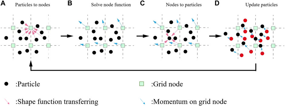
FIGURE 1. Computational cycle for the standard Material Point Method. (A) Map information from particles to grid nodes. (B) Solve node function. (C) Remap information to particles. (D) Update velocity and position of particles.

The continuous time is discretized by the central difference method, so Eq. 7 is expressed as the form of time integration in each time step:

p_{i I}^{n + 1 / 2} = p_{i I}^{n - 1 / 2} + f_{i I}^{n} Δ t (10)

where, $Δ t$ represents the increment of each time step which is a constant value in the paper, superscript represents the time step, and $p_{i I}^{n + 1 / 2}$ represents the resultant force of node force at the nth time step.

2.2 Computational cycle for MPM

The calculation cycle of MPM is shown in Figure 1. At each time step, the background grid is reset, and the information of the MPs is mapped to the grid node, as shown in Figure 1A; the grid node uses the information to solve the governing equation, and the constitutive equation is solved on the MPs, as shown in Figure 1B; then, the information solved on the grid node is mapped back to the MPs, as shown in Figure 1C; finally, update the MPs and discard the deformed grid, as shown in Figure 1D. The first, second, and third stages can be regarded as the Lagrangian stage, and the last stage can be regarded as the Euler stage.

Compared with the FEM, the computational grid of the FEM is permanently fixed with the object, while the background grid of the MPM is only fixed with the object in each time step, and at the end of each time step, the deformed grid is discarded. The MPs have carried all the information of the object. At the next time step, the information of the MPs is mapped to the background grid node through the shape function to determine the grid information. Therefore, no information of the grid node at each time is required to be recorded in the MPM. For large deformation problems, the FEM will reduce the accuracy due to grid distortion and produce numerical solution difficulties. The MPM will not encounter the problem that the calculation caused by grid distortion cannot be carried out, so it is very suitable for the simulation analysis of large deformation problems (Soga et al., 2018; Ying et al., 2021).

The momentum at the beginning of the time step is used to update the stress, that is, the USF format (Bardenhagen et al., 2001). The main advantages of the USF format are: first, the USF format has good stability and energy conservation characteristics; second, the USF format has a small amount of calculation. The specific calculation process is as follows:

Establish a new background grid, map the mass and momentum of the MPs to the grid nodes, and solve the node velocity:

m_{I}^{n} = \sum_{p} m_{p} N_{I p}^{n} (11)

P_{i I}^{n - 1 / 2} = \sum_{p} N_{I p}^{n} m_{p} v_{i p}^{n - 1 / 2} (12)

v_{i I}^{n - 1 / 2} = \frac{p_{i I}^{n - 1 / 2}}{m_{I}^{n}} (13)

Use the node velocity gradient to solve the strain rate ${\dot{ε}}_{i j p}^{n - 1 / 2}$ and rotation rate $Ω_{i j p}^{n - 1 / 2}$ of MPs, and then update the density and stress of each MP:

{\dot{ε}}_{i j p}^{n - 1 / 2} = \sum_{I} \frac{1}{2} (N_{I p, j}^{n} v_{i I}^{n - 1 / 2} + N_{I p, i}^{n - 1 / 2} v_{j I}^{n - 1 / 2}) (14)

Ω_{i j p}^{n - 1 / 2} = \sum_{I} \frac{1}{2} (N_{I p, j}^{n} v_{i I}^{n - 1 / 2} - N_{I p, i}^{n - 1 / 2} v_{j I}^{n - 1 / 2}) (15)

ρ_{p}^{n + 1} = ρ_{p}^{n} / (1 + {\dot{ε}}_{i j p}^{n - 1 / 2} Δ t) (16)

The stress update adopts the return mapping algorithm. The elastic trial stress ${\tilde{σ}}_{i j p}^{n}$ is first calculated according to the elastic constitutive model and then checked by the Drucker-Prager criterion. The stress exceeding the yield surface is pulled back to the yield surface to obtain the actual stress $σ_{i j p}^{n}$ .

The internal force and external force of nodes are calculated according to Eqs 8, 9, and the node momentum is updated by Eq. 10.

The incremental node velocity is mapped back to the MP by the FLIP momentum mapping scheme, and the position of the material point is updated:

v_{i p}^{n + 1 / 2} = v_{i p}^{n - 1 / 2} + Δ t^{n} \sum_{I} \frac{N_{I p}^{n} f_{i I}^{n}}{m_{I}^{n}} (17)

x_{i p}^{n + 1 / 2} = x_{i p}^{n} + Δ t^{n + 1 / 2} \sum_{I} \frac{N_{I p}^{n} P_{i I}^{n + 1 / 2}}{m_{I}^{n}} (18)

2.3 Contact algorithm

In order to avoid the adhesion of rocks when they are close, this paper employs the contact algorithm (Bardenhagen et al., 2001; Remacle et al., 2012) to separate them. Considering two approaching objects r and s, the contact criterion is:

(v_{i I}^{r} - v_{i I}^{s}) n_{i I}^{r} > 0 (19)

where, $n_{i I}^{r}$ represents the outer normal unit vector of the boundary of object $r$ at node $I$ . To make it satisfy the collinear condition, $n_{i I}^{r}$ is taken as

n_{i I}^{r} = - n_{i I}^{s} = \frac{{\hat{n}}_{i I}^{r} - {\hat{n}}_{i I}^{s}}{| {\hat{n}}_{i I}^{r} - {\hat{n}}_{i I}^{s} |}, n_{i I}^{r} = \frac{\sum_{p} m_{p} N_{I p, i}}{| \sum_{p} m_{p} N_{I p, i} |} (20)

When calculating the contact force of the node, the node momentum is updated independently according to the calculation method of the original MPM without considering the contact, denoted as the test momentum ${\hat{p}}_{i I}^{b, n + 1 / 2}$ ; then, the contact is judged according to Eq. 19. When the contact condition is not satisfied, the testing momentum is the real momentum. If the contact criterion is satisfied, the contact force is solved according to the continuous condition of the velocity field.

f_{i I}^{r, c, k} = \frac{1}{(m_{I}^{r, n} + m_{I}^{s, n}) Δ t} (m_{I}^{r, n} {\hat{p}}_{i I}^{s, n + 1 / 2} - m_{I}^{s, n} {\hat{p}}_{i I}^{r, n + 1 / 2}) (21)

The contact force of sliding contact is

f_{i I}^{b, c, k} = f_{i I}^{b, n o r, k} + μ ‖ f_{i I}^{b, n o r, k} ‖ \frac{f_{i I}^{b, \tan, k}}{‖ f_{i I}^{b, n o r, k} ‖} (22)

where, $f_{i I}^{b, n o r, n} = f_{i I}^{b, c, n} n_{j I}^{b, n} n_{i I}^{b, n}$ , is the normal contact force, $f_{i I}^{b, \tan, n} = f_{i I}^{b, c, n} - f_{i I}^{b, n o r, n}$ , is the tangential contact force, and then the contact force is used to correct the node momentum to obtain the real momentum $p_{i I}^{b, n + 1 / 2}$ ; the subsequent calculation process is still carried out according to Section 2.2.

3 Model

The geometric size of the model is shown in Figure 2A. The grey disc represents the block stone, and there are 83 blocks in the soil-rock mixed slope model, with the minimum diameter of 0.2 m and the maximum diameter of 1.6 m. The discrete model of material points is shown in Figure 2B. The edge length of the background grid is set to 0.1 m, and four material points are arranged in each grid. The spacing between the internal material points is 0.5 grid lengths, and the material point of the boundary is 0.25 grid lengths from the boundary. A total of 53636 material points are in total. The soil and the block stone account for 38750 and 14886, respectively, and the stone content is 27.75%. In the simulation, essential boundary conditions are applied on both sides, and the bottom of the model and other surfaces are free. The mechanical parameters of the material are shown in Table 1. The parameters are mainly from Zhao and Evan, (2009). The Young’s modulus of the rock is 400 times that of the soil, the ratio of the internal friction angle to the dilatancy angle is less than twice, and the ratio of the internal friction force is 30 times. In the actual simulation process, the rock will not reach the plastic state.

FIGURE 2

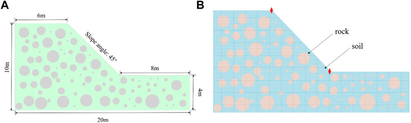
FIGURE 2. (A) Geometric parameters of SRM slope model. (The red marked points are the monitoring points of the shoulder and foot of the slope) (B) Discrete model of slope by MPs. (53636 material points in total, 38750 MPs for soil, 14886 MPs for stone).

TABLE 1

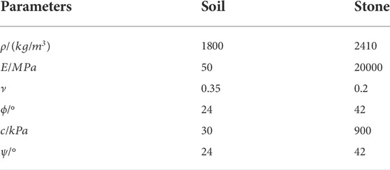
TABLE 1. Mechanical parameters of the SRM slope.

To make the simulation more stable, this paper sets a small-time step, 0.01 ms, in the simulation. The simulation process lasted for 12 s, which was divided into two stages. 0–2 s was the first stage, and a stable PIC momentum mapping format and elastic constitutive model were adopted. The gravity is linearly loaded until g = 9.8 m/s2, and then the momentum is set to 0 to obtain the initial state of the slope. 2–12 s is the second stage, using a FLIP momentum mapping scheme with good momentum conservation characteristics (Jiang et al., 2020), adopting the D-P criterion to calibrate the stresses.

4 Simulation results

MPM simulation was carried out based on the material point model in Figure 2B and the mechanical parameters in Table 1; the distribution of shear bands is shown in Figure 3.

ε_{v} = t r (ε) (23)

ε_{q} = ε - I ε_{v} (24)

ε_{q} = ε - I ε_{v} (25)

FIGURE 3

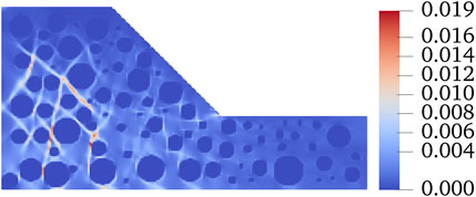
FIGURE 3. Shear zone distribution.

In the above equations, $ε$ , $ε_{v}$ and $ε_{q}$ represent strain, volume strain, and partial strain, $I$ represents unit matrix consistent with the strain tensor dimension, and $e$ represents generalized deviatoric strain.

In Figure 3, the dark blue circular area is stone, and the other areas are soil. It can be found that the shear failure area is mainly located at the bottom of the slope, and their distribution has a strong correlation with the distribution of stones. Compared with the regular distribution of arc plastic zone of homogeneous soil slope, the distribution of shear bands of SRM slope shows multiple interlaced effects. These shear bands are around the rock showing a strong correlation with the distribution of rock. Consistent with the report of Xu et al. (2008), the shear band distribution calculated in this paper can also be divided into three types, namely, the shear band distributed along the side of the block, the closed shear band distributed along both sides of the block and the non-closed shear band distributed along both sides of the block. In summary, the reliability of MPM in simulating SRM slope is sufficient. In the later part of this section, the soil properties of SRM slope are reduced to explore the influence of its properties on the stability of SRM slope.

4.1 Development of shear bands with decreasing cohesion

Figure 4 shows the development of the SRM slope shear zone with the decrease in soil cohesion.

FIGURE 4

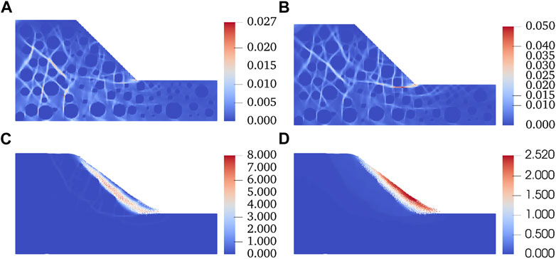
FIGURE 4. Development of shear bands with decreasing $c$ . (A) Distribution of shear band at the cohesion of 20 kPa. (B) Distribution of shear band at the cohesion of 10 kPa. (C) Distribution of shear band at the cohesion of 1 kPa. (D) Distribution of displacement (m) at the cohesion of 1 kPa.

When the cohesion decreases by 10 kPa, as shown in Figure 4A, the maximum shear deformation increases to 0.027, the shear deformation develops further, the shear zone expands gradually, and the shear zone below the slope develops most violently. The shear zone at the toe of the slope gradually penetrates the slope, and the internal shear zone gradually expands to the surface of the slope. However, at this time, the maximum shear deformation area is still distributed in the slope.

When the cohesion decreases by 20 kPa, see Figure 4B, currently, more shear bands extend to the slope surface and top, and the maximum shear deformation increases to 0.05, almost twice as much as Figure 4A. There are two main differences from the results in Figure 4A. First, the maximum shear deformation area is no longer inside the slope, but at the foot of the slope, and the shear deformation degree at the slope angle is much larger than that inside the slope. Second, the range of shear deformation is extended to the bottom of the slope and runs through the slope surface.

When the cohesion is reduced to 1 kPa, see Figure 4C, the primary shear zone is formed at this time, which is located on the slope surface, and a shallow landslide occurs. In addition, there is also a shear band that runs through the slope toe to the top of the slope, forming a potential sliding band. Between the two prominent shear bands, many shear bands are distributed around the block stones that connect them.

Figure 4D shows the displacement map when the cohesion is reduced to 1 kPa. The main sliding area is the soil at the slope surface, and the maximum displacement reaches 2.52 m. In addition, the rock and soil between the two main shear bands have an overall sliding, and the displacement value is about 0.5 m. The sliding surface is similar to the circular failure surface of the homogeneous soil slope.

4.2 Shear band with internal friction angle down

Figure 5 shows the development of the SRM slope shear zone with the soil internal friction angle decrease.

FIGURE 5

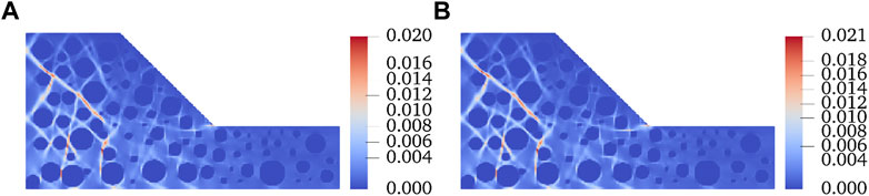
FIGURE 5. Development of shear bands with decreasing $ϕ$ . (A) Distribution of shear band at the angle of 20°. (B) Distribution of shear band at the cohesion of 16°.

When the internal friction angle drops to 20°, the distribution of shear deformation is shown in Figure 5A. From the perspective of the magnitude of shear deformation, compared with Figure 3, the maximum shear deformation increases by only 0.01, and the shear zones inside the slope are further developed. The shear zones with the maximum shear deformation are still those inside the slope, but their lengths are further extended and extend to the top of the slope. The development of the shear zone at the toe of the slope is apparent: compared with Figure 3, it can be found that the shear zone at the toe of the slope gradually extends into the slope surface; a series of interlaced small shear zones are gradually formed under the slope.

When the internal friction angle drops to 16°, the shear deformation map is shown in Figure 5B. Compared with the size of shear deformation, the maximum shear deformation still does not increase significantly. Compared with Figure 5A, the size and distribution of shear deformation are almost the same. Therefore, it can be said that the decrease in internal friction angle has little effect on the stability of the SRM slope.

4.3 Shear bands develop with the decrease of cohesion and internal friction angle

Figure 6 shows the development of the SRM slope shear zone with the decrease of soil friction angle and cohesion.

FIGURE 6

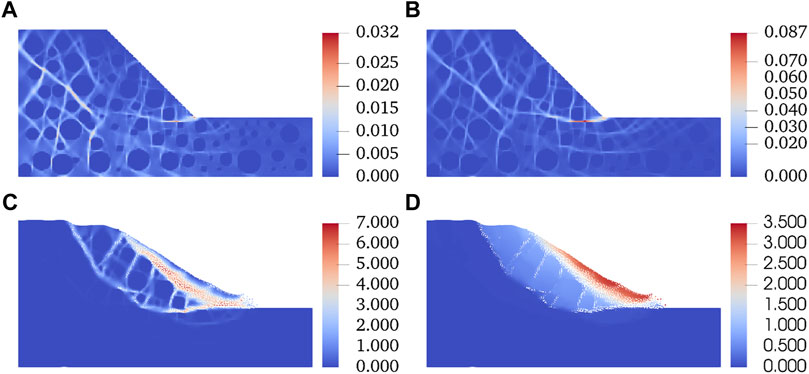
FIGURE 6. Shear bands develop with the decrease of $c$ and $ϕ$ . (A) Distribution of shear bands at $ϕ = 20^{\circ}$ and $c = 20$ kPa. (B) Distribution of shear bands at $ϕ = 20^{\circ}$ and $c = 10$ kPa. (C) Distribution of shear bands at $ϕ = 20^{\circ}$ and $c = 1$ kPa. (D) Distribution of displacement (m) at $ϕ = 20^{\circ}$ and $c = 1$ kPa.

Figure 6A shows the simulation results when the cohesion is 20 kPa, and the internal friction angle is 20°. Compared with Figure 3, the shear deformation develops rapidly, and the maximum value increases to 0.032. The maximum shear deformation areas are mainly located at the toe and inside the slope and extend to the top and surface. The shear band inside the slope extends to the rock and soil mass at the bottom of the slope.

When the cohesive force is 10 kPa, and the internal friction angle is 20°, the simulation results are shown in Figure 6B. At this point, multiple shear bands extend to the slope surface and top. Compared with Figure 3, the maximum shear deformation increases to 0.087, which is 4.6 times higher. The results are different from those in Figure 6A in three aspects: first, the maximum shear deformation area is no longer inside the slope but at the foot of the slope, and the shear deformation degree at the slope angle is much larger than that inside the slope; second, the range of shear deformation is extended to a farther position at the bottom of the slope and runs through the surface of the bottom of the slope; third, the shear zone at the foot of the slope runs through the slope and extends to the top of the slope, forming a primary shear zone, and many shear zones run through the top of the slope are also formed within the slope.

When the cohesion is 1 kPa, and the internal friction angle is 20°, the simulation results are shown in Figure 6C. At this time, two main shear bands are formed, one near the slope, the other runs through the slope toe to the top of the slope, and many shear bands are distributed around the rocks that connect them. Figure 6D shows the displacement map currently; the displacement of the soil near the slope is the largest, reaching 3.5 m; the integrity of the rock and soil mass between the two shear bands is good, and the circular sliding occurs. The displacement of this part is about 1.5 m, and the displacement is almost unchanged in this region.

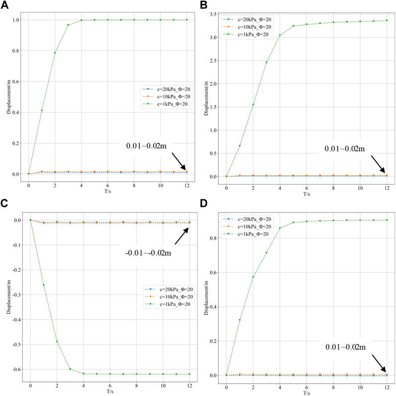
Figure 7 shows the displacement variation of the monitoring points with the decrease of soil friction angle and cohesion. According to Figure 7A and Figure 7C, the displacement as well as the vertical displacement of the slope shoulder changes very slightly until the nature of the matrix is reduced to c = 1 kPa, $ϕ$ = 20°. Meanwhile, according to Figure 7B and Figure 7D, we can find that the displacement as well as the vertical displacement of the slope foot also changes very slightly, and the displacement magnitude are basically the same as the slope shoulder. It proves that the slope body has good integrity.

FIGURE 7

FIGURE 7. The displacement variation curve of the monitoring points. (A) Displacement variation curve of the slope shoulder. (B) Displacement variation curve of the slope foot. (C) Vertical displacement variation curve of the slope shoulder. (D) Vertical displacement variation curve of the slope foot.

When the property of the matrix was reduced to c = 1 kPa, $ϕ$ = 20°, the displacements of both the shoulder and the foot of the slope changed abruptly, and the change of the foot of the slope was a bit larger, which was mainly caused by the strong mobility of the matrix at this stage. From the change of vertical displacement, the vertical displacement of the slope foot is slightly larger than that of the shoulder of the slope, which is since the stones slide toward the foot of the slope in the process of landslide and keep a whole without destruction all the time, so the soil around them is raised up by the stones.

Figure 8 shows the velocity cloud at different times with cohesion of 1 kPa and internal friction angle of 20°. The duration of the landslide is about 5 s. At 1s, the maximum rate is about 0.8 m/s, mainly distributed in a very shallow soil layer on the slope surface, and the SRM rate under the surface is about 0.3 m/s. At 2 s, the rate of landslide reaches the maximum, reaching 1 m/s, and the rate of SRM under the slope surface is still maintained at about 0.3 m/s. At 3 s, the soil slid to the bottom of the slope, the rate decreased and gradually accumulated, and the lower SRM rate closed to 0. The slope returned to a stable state in 5 s. By comparing the rate maps at each time, it can be found that the maximum rate is always distributed in the soil on the slope surface; the speed of SRM has almost no change in the sliding process and presents the characteristics of uniform distribution.

FIGURE 8

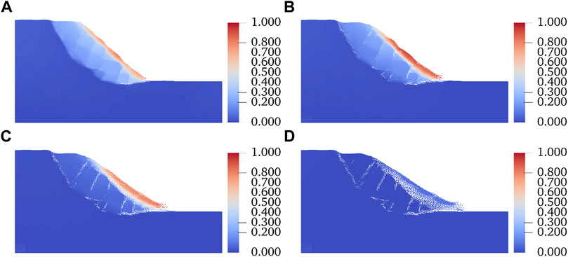
FIGURE 8. Slope velocity (m/s) map. (A) Sliding time t = 1 s. (B) Sliding time t = 2 s. (C) Sliding time t = 3 s. (D) Sliding time t = 5 s.

5 Discussion

In this paper, the effect of slope matrix on the SRM slope deformation behavior is studied based on MPM. The cohesion and internal friction angle of the soil were analyzed parametrically, respectively, and the deformation response of the slope was investigated when both of them were reduced simultaneously. However, there are some shortcomings in this study, which need to be optimized, and they were discussed in the following.

1) In actual engineering, the distribution and morphology of stones of SRM slopes are highly random. In this paper, when conducting the research, only round stones were selected for the study due to the limitation of calculation ability. In the future, we should set the stone distribution more in line with the engineering reality for research, or analyze the simulation results by means of artificial intelligence, which may be able to get some guiding results, which are self-evident to the practical engineering.

2) In this paper, when reducing the cohesion and internal friction angle of soil, the correlation between the two is not considered, but the values of both are mechanically reduced, which may lead to some unreasonable results. A more reliable research work can be carried out by using the principle of strength reduction or establishing the MPM framework of fluid-solid coupling to consider the effect of water on soil properties.

3) Stones are very critical to the stability of SRM slopes, and the deformation of stones during landslides was not considered in this paper. In the future, an algorithm can be set up to track the movement of the stones during the landslide, and next, a crack extension algorithm can be set up to be able to track the cracking of the stone blocks.

6 Conclusion

Based on MPM, the stability of SRM and the large deformation stage after instability are simulated. Firstly, the SRM slope model with circular stones of different diameters is established, and then its stability is analyzed by MPM, and the following main conclusions are obtained.

(1) The establishment of the SRM model of the MPs is relatively simple. The MPs carry all the information of MPM, and When establishing the model, the corresponding SRM model can be obtained by giving different properties to the material points representing the stone and the soil. Comparing with other methods, the calculation results of MPM have high reliability, which proves the effectiveness of MPM in analyzing SRM problems.

(2) By comparing the influence of different matrix properties on the stability of SRM, it is found that the decrease of cohesion has a more significant influence on the stability of SRM than the internal friction angle. When the two are reduced simultaneously, the shear band expands rapidly and enters the stage of large deformation.

(3) When the SRM slope is unstable, and then large deformation occurs, the sliding mode of the surface soil is translational. In contrast, the geomaterial below the slope shows good integrity, and the sliding mode is rotation.

Data availability statement

The data analyzed in this study is subject to the following licenses/restrictions: All data, models, or code generated or used during the study are available from the corresponding author by request. Requests to access these datasets should be directed to Yong Zheng, zhengyong@cqjtu.edu.cn.

Author contributions

XL: resources, data curation, and project; ST: software; YZ: writing—original draft preparation; JL, and LW: resources, data curation, and project; KH: validation and investigation; TJ: editing.

Funding

This work is financially supported by the National Natural Science Foundation of China (No. 52108304), and the China Postdoctoral Science Foundation (No. 2022M710540).

Conflict of interest

Authors JL and LW are employed by Chongqing Water Conservancy and Electric Power Survey and Design Institute Co., Ltd.

The remaining authors declare that the research was conducted in the absence of any commercial or financial relationships that could be construed as a potential conflict of interest.

Publisher’s note

All claims expressed in this article are solely those of the authors and do not necessarily represent those of their affiliated organizations, or those of the publisher, the editors and the reviewers. Any product that may be evaluated in this article, or claim that may be made by its manufacturer, is not guaranteed or endorsed by the publisher.

References

Bardenhagen, S. G., Guilkey, J. E., Roessig, K. M., Brackbill, J. U., Witzel, W. M., and Foster, J. C. (2001). An improved contact algorithm for the material point method and application to stress propagation in granular material. CMES - Comput. Model. Eng. Sci. 2 (4), 509–522. doi:10.3970/cmes.2001.002.509

CrossRef Full Text | Google Scholar

Bardenhagen, S. G., Kober, E. M., et al. (2004). The generalized interpolation material point method. CMES - Comput. Model. Eng. Sci. 5 (6), 477–595. doi:10.3970/cmes.2004.005.477

CrossRef Full Text | Google Scholar

Bono, J. d., Mcdowell, G., and Wanatowski, D. (2012). Discrete element modelling of a flexible membrane for triaxial testing of granular material at high pressures. Geotech. Lett. 2 (4), 199–203. doi:10.1680/geolett.12.00040

CrossRef Full Text | Google Scholar

Chen, Z., and Brannon, R. (2002). An evaluation of the material point method. New Mexico: Sandia National Laboratories, 46. doi:10.2172/793336

CrossRef Full Text | Google Scholar

Cil, M. B., and Alshibli, K. A. (2014). 3D analysis of kinematic behavior of granular materials in triaxial testing using DEM with flexible membrane boundary. Acta Geotech. 9 (2), 287–298. doi:10.1007/s11440-013-0273-0

CrossRef Full Text | Google Scholar

Coli, N., Berry, P., and Boldini, D. (2011). In situ non-conventional shear tests for the mechanical characterisation of a bimrock. Int. J. Rock Mech. Min. Sci. 48 (1), 95–102. doi:10.1016/j.ijrmms.2010.09.012

CrossRef Full Text | Google Scholar

Cui, S., Pei, X., Jiang, Y., Wang, G., Fan, X., Yang, Q., et al. (2021). Liquefaction within a bedding fault: Understanding the initiation and movement of the Daguangbao landslide triggered by the 2008 Wenchuan Earthquake (Ms = 8.0). Eng. Geol. 295 (20), 106455. doi:10.1016/j.enggeo.2021.106455

CrossRef Full Text | Google Scholar

Graziani, A., Rossini, C., and Rotonda, T. (2012). Characterization and dem modeling of shear zones at a large dam foundation. Int. J. Geomech. 12 (6), 648–664. doi:10.1061/(ASCE)GM.1943-5622.0000220

CrossRef Full Text | Google Scholar

He, Y., and Kusiak, A. (2017). Performance assessment of wind turbines: Data-derived quantitative metrics. IEEE Trans. Sustain. Energy 9 (1), 65–73. doi:10.1109/TSTE.2017.2715061

CrossRef Full Text | Google Scholar

Jiang, Y., Li, M., Jiang, C., and Alonso-Marroquin, F. (2020). A hybrid material-point spheropolygon-element method for solid and granular material interaction. Int. J. Numer. Methods Eng. 121 (14), 3021–3047. doi:10.1002/nme.6345

CrossRef Full Text | Google Scholar

Li, H., Deng, J., Feng, P., Pu, C., Arachchige, D., and Cheng, Q. (2021a). Short-term nacelle orientation forecasting using bilinear transformation and ICEEMDAN framework. Front. Energy Res. 9, 780928. doi:10.3389/fenrg.2021.780928

CrossRef Full Text | Google Scholar

Li, H., Deng, J., Yuan, S., Feng, P., and Arachchige, D. (2021b). Monitoring and identifying wind turbine generator bearing faults using deep belief network and EWMA control charts. Front. Energy Res. 9, 799039. doi:10.3389/fenrg.2021.799039

CrossRef Full Text | Google Scholar

Li, H., He, Y., Xu, Q., Deng, j., Li, W., and Wei, Y. (2022). Detection and segmentation of loess landslides via satellite images: A two-phase framework. Landslides 9, 673–686. doi:10.1007/s10346-021-01789-0

CrossRef Full Text | Google Scholar

Liang, W., and Zhao, J. (2019). Multiscale modeling of large deformation in geomechanics. Int. J. Numer. Anal. Methods Geomech. 43 (5), 1080–1114. doi:10.1002/nag.2921

CrossRef Full Text | Google Scholar

Remacle, J., Lambrechts, J., Seny, B., Marchandise, E., Johnen, A., and Geuzainet, C. (2012). Blossom‐quad: A non‐uniform quadrilateral mesh generator using a minimum‐cost perfect‐matching algorithm. Int. J. Numer. Methods Eng. 89 (9), 1102–1119. doi:10.1002/nme.3279

CrossRef Full Text | Google Scholar

Soga, K., Alonso, E., Yerro, A., Kumar, K., and Bandara, S. (2018). Trends in large-deformation analysis of landslide mass movements with particular emphasis on the material point method. Geotechnique 66 (3), 248–273. doi:10.1680/jgeot.15.LM.005

CrossRef Full Text | Google Scholar

Sulsky, D., Chen, Z., and Schreyer, H. L. (1994). A particle method for historydependent materials. Comput. Methods Appl. Mech. Eng. 118 (1 2), 179–196. doi:10.1016/0045-7825(94)90112-0

CrossRef Full Text | Google Scholar

Xu, W., Yue, Z., and Hu, R. (2008). Study on the mesostructure and mesomechanical characteristics of the soil-rock mixture using digital image processing based finite element method. Int. J. Rock Mech. Min. Sci. 45 (5), 749–762. doi:10.1016/j.ijrmms.2007.09.003

CrossRef Full Text | Google Scholar

Yilmaz, I., Marschalko, M., Bednarik, M., Kaynar, O., and Fojtova, L. (2012). Neural computing models for prediction of permeability coefficient of coarse-grained soils. Neural comput. Appl. 21 (5), 957–968. doi:10.1007/s00521-011-0535-4

CrossRef Full Text | Google Scholar

Ying, C., Zhang, K., Wang, Z. N., Siddiqua, S., Makeen, G. M. H., and Wang, L. (2021). Analysis of the run-out processes of the xinlu village landslide using the generalized interpolation material point method. Landslides 18 (4), 1519–1529. doi:10.1007/s10346-020-01581-6

CrossRef Full Text | Google Scholar

Yue, Z. Q., and Morin, I. (1996). Digital image processing for aggregate orientation in asphalt concrete mixtures. Can. J. Civ. Eng. 23 (2), 480–489. doi:10.1139/l96-052

CrossRef Full Text | Google Scholar

Zhao, X., and Evans, T. (2009). Discrete simulations of laboratory loading conditions. Int. J. Geomech. 9 (4), 169–178. doi:10.1061/(asce)1532-3641(2009)9:4(169)

CrossRef Full Text | Google Scholar

Zhou, J., Wei, J., Yang, T., Zhang, P., Liu, F., and Chen, J. (2021). Seepage channel development in the crown pillar: Insights from induced microseismicity. Int. J. Rock Mech. Min. Sci. 145, 104851. doi:10.1016/j.ijrmms.2021.104851

CrossRef Full Text | Google Scholar

Keywords: soil-rock mixture, matrix, material point method, large deformation, sliding mode

Citation: Li X, Tang S, Zheng Y, Liu J, Wang L, He K and Jiang T (2022) Influence of the matrix of the soil-rock mixture on deformation and failure behaviors of the slope based on material point method. Front. Earth Sci. 10:997928. doi: 10.3389/feart.2022.997928

Received: 19 July 2022; Accepted: 22 August 2022;
Published: 13 September 2022.

Edited by:

Jingren Zhou, Sichuan University, China

Reviewed by:

Feng Li, Shenzhen University, China
Chaofan Liu, Tongji University, China

Copyright © 2022 Li, Tang, Zheng, Liu, Wang, He and Jiang. This is an open-access article distributed under the terms of the Creative Commons Attribution License (CC BY). The use, distribution or reproduction in other forums is permitted, provided the original author(s) and the copyright owner(s) are credited and that the original publication in this journal is cited, in accordance with accepted academic practice. No use, distribution or reproduction is permitted which does not comply with these terms.

*Correspondence: Yong Zheng, zhengyong@cqjtu.edu.cn

ORIGINAL RESEARCH article

Influence of the matrix of the soil-rock mixture on deformation and failure behaviors of the slope based on material point method

1 Introduction

2 Methodology

2.1 Governing equation and discretization

2.2 Computational cycle for MPM

2.3 Contact algorithm

3 Model

4 Simulation results

4.1 Development of shear bands with decreasing cohesion

4.2 Shear band with internal friction angle down

4.3 Shear bands develop with the decrease of cohesion and internal friction angle

5 Discussion

6 Conclusion

Data availability statement

Author contributions

Funding

Conflict of interest

Publisher’s note

References

This article is part of the Research Topic

People also looked at