Gas production prediction and risk quantification of shale gas reservoirs in Sichuan Basin based on Gauss prediction model and Monte Carlo probability method

Introduction

In recent years, China’s natural gas industry has been developing rapidly, its consumption has been growing rapidly, and its importance in the national energy system has been increasing (Du et al., 2021). Natural gas production prediction and risk quantification are very important parts of gas field development planning and the core work of gas field development planning, which plays an important macro guiding role in the realization of gas field development planning and production index. At present, the research work of long-term production growth forecast and risk quantification of oil and gas has been carried out widely in the world. Countries all over the world attach great importance to the research work of oil and gas resource growth prediction and risk quantification (Zhang and Rong, 2007).

In Sichuan Basin, shale gas is in the early and middle stage of resource exploration. Shale gas reservoirs have strong resource base and great potential of exploration and development, which can greatly promote the increase of natural gas production and benefit in Sichuan Basin (Li et al., 2015; Wang 2022).

However, the shale gas reservoir has strong reservoir heterogeneity, complex pressure system and other geological characteristics, which is not conducive to determine the future production scale of the gas reservoir. At the same time, determining production scale through reasonable research methods is the key to efficient development of gas reservoirs (Li et al., 2019; Xie et al., 2021). Therefore, strengthening the research work of shale gas production growth prediction and risk quantification in Sichuan Basin can further clarify the resource exploration and development potential in this field. Furthermore, it has an important guiding role for shale gas production planning in this area.

There is many research on prediction models of natural gas storage and production, such as peak prediction method, neural network method, grey system method, etc. (Huang et al., 2011; Lu et al., 2021). Among them, neural network method is the most widely used method for predicting medium - and long-term natural gas production (Liang et al., 2020; Wang et al., 2020; Hu, 2022). For the natural gas areas that are still in the early development stage or the upper production stage, the reservoir numerical simulation method is used to predict the natural gas storage and production in the medium and long term, which has higher accuracy and is more practical (Liu et al., 2020; Zhang L. et al., 2021). Based on the new DAR method, Deng et al., 2022 used multiple regression to establish dimensionless pseudo-correlation function of independent variables of temperature and pressure, and constantly modified the equation, and proposed a new calculation formula of deviation coefficient for ultra-deep HHT gas reservoirs. The research results can provide a reference for accurately calculating the early dynamic reserves of ultra-deep HP/HT gas reservoirs. Ye and Xue, 2009 established a prediction model for oil and gas resources production and development in China by using nonlinear exponential regression model and model method in grey system theory. Qiao et al., 2021, taking Qinshui Basin as the research area, established a grey prediction model to predict the gas production change of COALbed methane reservoir, and verified the actual gas production data, and concluded that the grey prediction model has a good prediction effect on the dynamic change of coalbed methane reservoir when gas production enters the decline stage. Zhou et al., 2008 used exponential smoothing method to process sample data and improved the calculation method of the background value of the grey model. Case analysis showed that the improved grey model had higher prediction accuracy.

At present, there are many research methods to quantify the risk of natural gas storage and production, including probability method, neural network method, fuzzy clustering method and so on (Shaolei et al., 2021; Zhang et al., 2020; Ma et al., 2021). Among them, probability method is widely used in the study of natural gas production risk quantification. For gas areas that are less explored and developed, the probability method can predict the probability of realization of different reservoir production targets in the future according to the existing data, which provides a reliable theoretical basis for the formulation of production planning schemes. Wang et al., 2020 established an improved multi-period generalized model based on the generalized model commonly used in the life cycle model method to determine the number of cycles in oil and gas field production prediction and improve the prediction effect of the model. The fitting effect of the improved model is better than that of single-period model and multi-period model. In order to quantitatively describe and analyze the risk of recoverable shale gas reserves, Chen et al., 2022 established a comprehensive evaluation model by using Monte Carlo simulation from the perspective of probability and statistics. The probability distribution is used to define the range of key technical and economic parameters, describe the range of shale gas recoverable reserves evaluation results, and reflect the actual development status of shale gas projects. Zhang P. et al., 2021 determined the distribution function of oil and gas reserve evaluation parameters by using probability method and conducted sensitivity analysis on each parameter, thus realizing the reserve evaluation of the whole gas field. The reserves of the whole gas field are predicted by arithmetic summation of each calculation unit. The proved reserves predicted by deterministic volume method are close to the Pmean reserves calculated by probability method.

Obviously, most of the research on natural gas production prediction and production risk quantification are two independent research contents. Therefore, the two research contents need to be combined, that is, production risk quantification research based on production prediction results can provide more quantitative basis for the guidance of natural gas exploration and development. In this paper, the final recoverable reserves (URR) are introduced into Hubbert and Gauss prediction model as the boundary condition, and the production prediction results of Sinian gas reservoir are obtained. The prediction accuracy of the two models is compared by correlation analysis. Monte Carlo simulation method was used to randomly extract the output of each year and calculate the probability p of production distribution and realization of each year. At the same time, it provides evaluation index for production risk grade evaluation by calculating dispersion degree C. The production risk of natural gas is systematically quantified through the self-built production grade evaluation matrix, which provide reliable planning basis for production target realization. The research process of shale gas production prediction and risk quantification is shown in Figure 1.

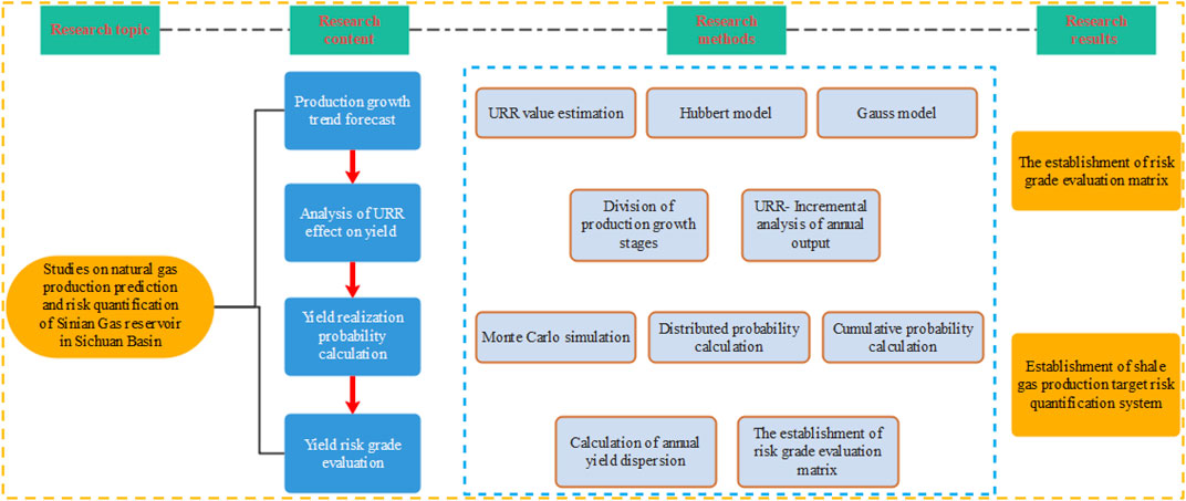
FIGURE 1. Flow chart of shale gas production prediction and risk quantification research.

Theory of shale gas production prediction and risk quantification

Theory of natural gas production prediction

Hubbert prediction model

Hubbert model is a common life cycle model for shale gas production peak prediction. This model mainly has the following characteristics (Zhou et al., 2018):

When the oil and gas field is put into development, the production starts to rise from 0, and gradually reaches the peak with the extension of development time. After that, production declines with the extension of development time until the resource are exhausted. As the development time approaches infinity, the area of the production curve and time is equal to the final recoverable reserves of the field. The Hubbert model equation is as follows:

Where, $P$ represents the cumulative output, in unit ${10}^8{m}^3/a$; $URR$ represents final recoverable reserves, unit ${10}^8{m}^3$; $t$ is the production and exploitation time, in unit of year; $t_n$ represents peak production time; b is a model parameter, which can represent the slope of the peak to a certain extent.

Take the derivative of formula (1) with respect to t, the calculation formula of annual output can be obtained.

Where, $Q$ represents the annual output in unit ${10}^8{m}^3/a$.

When $t=t_n$, production growth reaches its peak. At this point, the change rate of cumulative output M is the largest, that is, $dM/dt$ is the largest:

In the formula, $Q_m$ is the peak annual production in unit of ${10}^8{m}^3/a$.

Transform formula (3) into $URR=4Q_m/b$ and substitute it into Formula (2). The calculation formula of annual output of Hubbert model can be obtained (Wang et al., 2016).

The curve of Hubbert model increases gently at the beginning, then a stable period is reached at the peak, and ultimately drops rapidly until the resources are completely exhausted.

Gauss prediction model

Gauss and Hubbert models both are growth curves obtained based on life cycles, and both present symmetric forms (Zhang et al., 2019; Zhou et al., 2021). The distribution density function of the Gauss model is:

In the formula, $\mu$ is the mean value; $s$ is the standard deviation.

The cumulative production within the interval of $\left(0-\infty \right)$ during production time t is defined as the final recoverable reserves URR, and the calculation formula of annual production can be obtained by multiplying the distribution density function $f\left(t\right)$ with the final recoverable reserves URR [27].

The derivative of Formula (6) is applied to the mining time t.

When the production growth reaches the peak, the annual production change rate $\frac{dQ}{dt}=0$.At this point.

By substituting $t_m=\mu$ into formula (6), the peak annual production $Q_m$ can be obtained.

By substituting formulas (8) and (9) into Formula (6), the calculation formula of annual output of Gauss model can be obtained.

In the formula, the model parameters s can represent the fluctuation of the peak to a certain extent.

Theory of quantifying production risk

Monte Carlo probability method

The basic idea of Monte Carlo probability method is to establish the calculation model of the probability of occurrence through the statistical characteristics of “sampling test,” and get the approximate results of the realization probability.

The specific steps of Monte Carlo probability method are as follows: Firstly, the solved problem is transformed into the expected value of a probability model, and then a computer simulation test is carried out to conduct random sampling of the model, extract enough random numbers, and conduct statistical analysis on the problem to be solved [28].

Suppose that the distribution density of random variable f (x) is ψ(x), then the mathematical expectation of variable f (x) is:

According to the distribution density function g(x), N sample points $x_i$ are randomly selected, and the arithmetic mean value of the function value $f\left(x_i\right)$ corresponding to the sample points is taken as the integral estimation value.

Monte Carlo simulation can realize the calculation process of variable random sampling. According to the probability distribution density function of the variable, the variable values are extracted randomly in turn, and the probability density distribution of the objective function can be obtained through many repeated independent simulation (Zhang S. et al., 2021).

It is the premise of Monte Carlo simulation to determine the mathematical model of objective function and the probability distribution of variables in the model. According to the given probability distribution parameters, many random samples are generated, and the probability density distribution curve of the objective function is calculated by the model. Figure 2 shows the specific calculation steps.

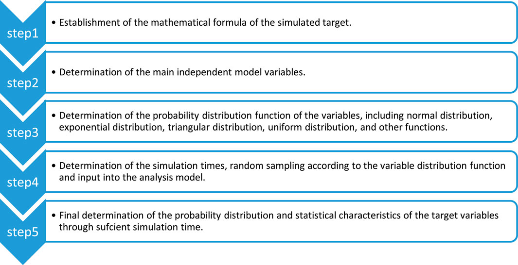
FIGURE 2. Monte Carlo method calculation steps.

Risk level evaluation matrix

Two indexes, realization probability p and production dispersion degree C, are need to evaluate the risk level of production. The discrete degree of output refers to the degree of difference between output values and other output values, that is, the degree of production change caused by the change of production risk factors (Gutierrez et al., 2016). Therefore, the smaller the value of dispersion degree C is, the less it is affected by risk factors, and the greater the stability of output is.

The calculation formula of dispersion degree is as follows:

In the formula, μ is the mean value and s is the standard deviation.

The establishment of risk assessment matrix requires comprehensive consideration of production realization probability p and dispersion degree C. According to the shale gas production prediction results, the production risk can be comprehensively quantified by referring to the four grades of production risk (Figure 3).

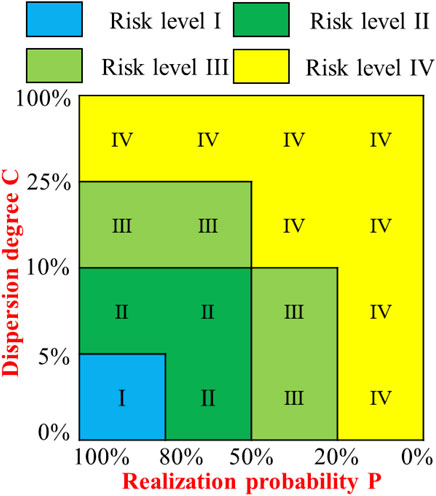
FIGURE 3. Production risk rating evaluation matrix.

The corresponding relationship between regions of output risk matrix and risk grade judgment criteria is shown in Figure 4.

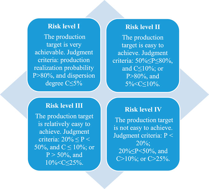
FIGURE 4. Risk grade judgment criteria.

Shale gas production projections

Estimate of final recoverable reserves (URR)

According to the shale gas production curve starting since 2011 (Figure 5), the exploration and development of shale gas in Sichuan Basin is relatively short. The trend of shale gas production curve maintaining rapid growth is consistent with the trend of Hubbert and Gauss prediction model (Eqs 4, 10) in the early growth stage of the curve. Therefore, these two prediction models can be used in the study of shale gas production prediction.

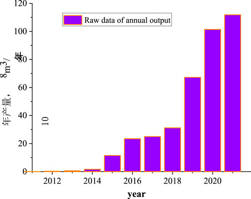
FIGURE 5. Annual production growth trend of shale gas.

Estimate the URR range of final recoverable reserves (hereinafter referred to as URR) is a prerequisite for shale gas production prediction. The rapid growth in shale gas production indicates that the resource is still in the early stages of exploration and development (Figure 5). Because of the short exploration and development time of shale gas, the cognition degree of gas reservoir is not enough. Therefore, URR is simply estimated by numerical method.

Geological exploration has proved that the resource of shale gas in Sichuan Basin is $31.14\times {10}^{12}{m}^3$. On the basis of analyzing the law of exploration and development of several gas reservoirs in Sichuan Basin, the appropriate exploration speed and recovery range of shale gas are selected. In the current technical conditions of shale gas exploration and exploitation, the proved rate of shale gas in Sichuan Basin is 15–25%, and the cumulative proved reserves at the end-of-life cycle are $\left(4.67-7.79\right)\times {10}^{12}{m}^3$. The current recovery factor of shale gas in the Sichuan Basin is about 20%, and the URR range is estimated to be $\left(9342-15570\right)\times {10}^8{m}^3$. It should be noted that with the deepening of the cognition of gas reservoir, the calculation method of URR also needs to be improved.

Shale gas production growth trend prediction

Hubbert and Gauss peak prediction models are used to predict 15%–25% peak shale gas production. The URR values corresponding to each exploration rate is calculated (Table 1), and the shale gas production growth trends under these five different detection rates is studied by selecting the discovery rates of 15%, 175%, 20%, 22.5% and 25%, respectively.

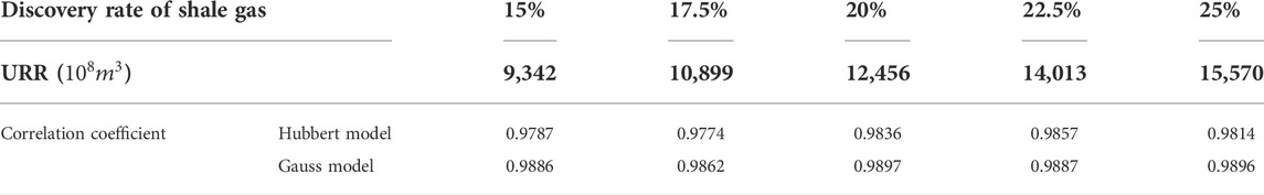
TABLE 1. Correlation analysis of production prediction results.

Different URR values are substituted into formulas (4) and (10), respectively, to obtain the shale gas production growth formulas (Formulas (14) and (15)) and shale gas production prediction results (Figure 6A and Figure 7A). Formula (14) is the output growth formula of Hubbert model, and Formula (15) is the output growth formula of Gauss model. The peak annual production $Q_m$, peak production time $t_m$, peak slope b, standard deviation s and other model parameters of the two formulas represent different URR conditions. These two formulas correspond to Figures 6A, 7A respectively.

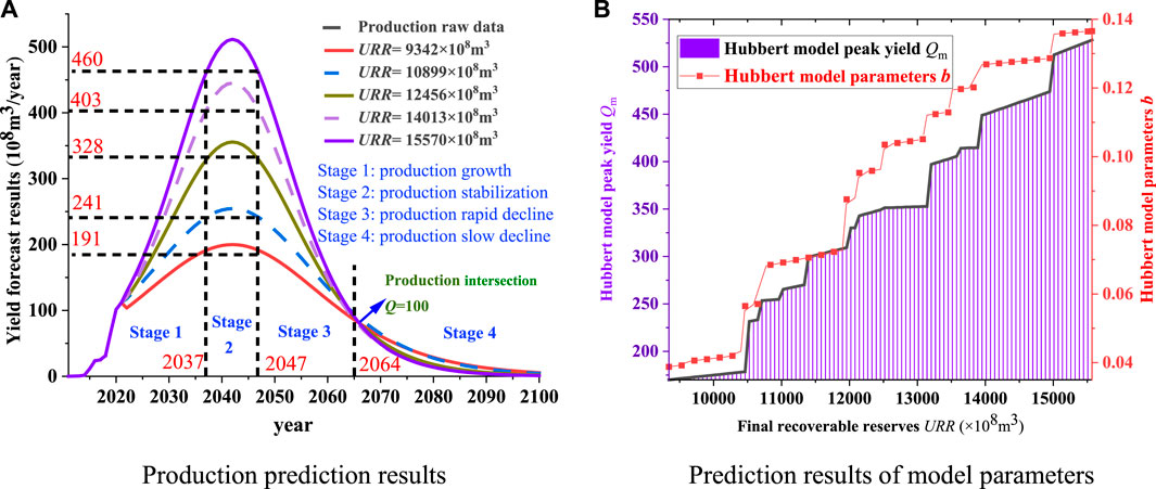
FIGURE 6. Prediction results of shale gas production based on Hubbert model. (A) Production prediction results. (B) Prediction results of model parameters.

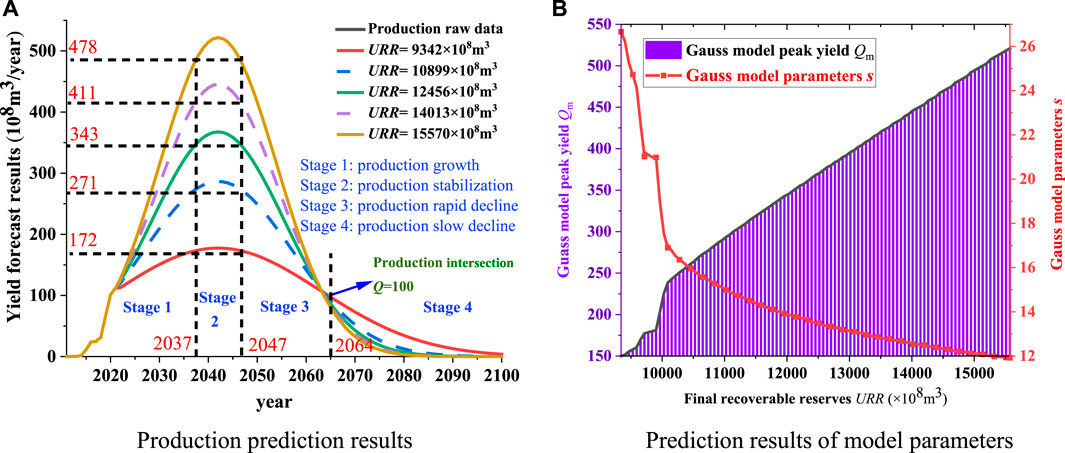
FIGURE 7. Prediction results of natural gas production based on Gauss model. (A) Production prediction results. (B) Prediction results of model parameters.

By studying the relationship between the above model parameters and URR, the growth law of shale gas production with URR can be further analyzed. In the estimated range $URR=\left(9342-15570\right)\times {10}^8{m}^3$, 100 different URR values are uniformly extracted. The above URR values are calculated by substituting them into formulas (4) and (10), and corresponding model parameter values (Figures 6B, 7B) are extracted through different production prediction results obtained (Figures 6A, 7A). In this paper, the production prediction results of five kinds of URR are selected to display, including the upper and lower boundary values of URR estimation range, to predict the boundary of future production.

It can be seen from Figures 6A, 7A that the production prediction results of the two models are highly similar and can be analyzed simultaneously. The production always reaches the peak in 2042 with the increase of URR, i.e. $t_m\equiv 2042$. During the period of 2022–2062, the production growth curve is axisymmetric with respect to t=2042.

In Figure 6B, with the increase of URR, the peak production $Q_m$ and parameter b of Hubbert model show a ladder growth trend. When the URR increases to a certain value, the parameter will increase rapidly, and then show a gentle increase. In Figure 7B, the output peak $Q_m$ of Gauss model increases linearly. With the increase of URR, the numerical curve of parameter s keeps a relatively smooth downward trend, and the decreasing rate gradually decreases. The variation of model parameters reflects the production variation. Therefore, when URR is at the same growth rate, Gauss model has a more stable yield growth trend than Hubbert model.

According to the production growth rate, the production growth process in the future period can be divided into four stages: the production rise stage (2022–2037), the production stability stage (2037–2047), the production rapid decline stage (2047–2064) and the production slow decline stage (2064–2090). In 2022–2037, the output is in a period of rapid annual growth. From 2037 to 2042, the output will keep steady growth and reach the peak $Q_m$ in 2042. From 2042 to 2047, the output will keep a steady decline. From 2047 to 2064, the production began to decrease rapidly with the increase of years. After 2064, the production curve begins to decline slowly and gradually approaches zero. Notably, the production curve converges in 2064 when annual yield is $Q=100\times {10}^8{m}^3$. Therefore, the year 2064 is regarded as the dividing line between the rapid decline stage and the slow decline stage.

By introducing the correlation analysis process, the accuracy of the two production prediction results can be compared. Correlation analysis was conducted between Hubbert model and historical data for five kinds of production prediction data, and the same with Gauss model. As shown in Table 1, the correlation coefficients of the two models are very close to 1, and the corresponding yield prediction results are very accurate. However, the correlation coefficients of Gauss model under the same URR are all higher than that of Hubbert model. Therefore, the prediction data of Gauss model with higher correlation coefficient are selected as the result of shale gas production prediction. The yield prediction results under different URR conditions are obtained (Table 2).

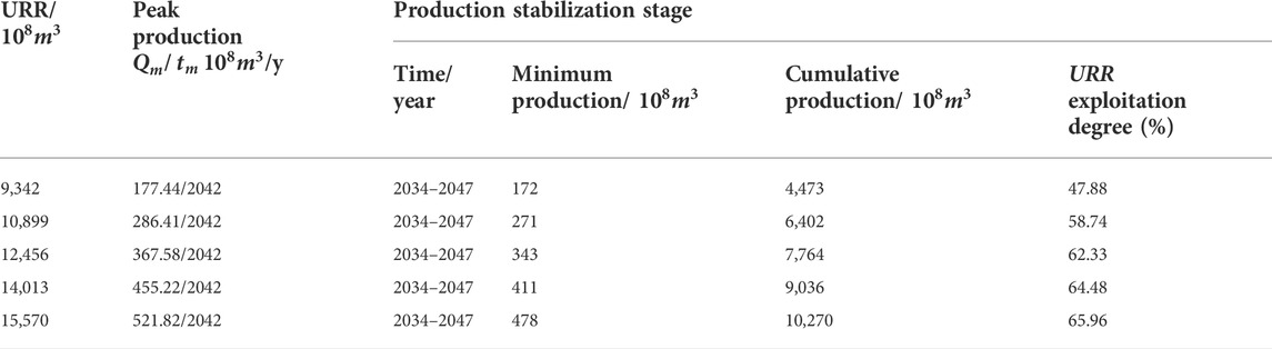
TABLE 2. Production prediction results of shale gas under different URR.

Comprehensive evaluation

The exploration and development of shale gas is relatively low and there are many unknown factors, so the URR of recoverable reserves eventually becomes the dominant factor affecting the production trend. The estimated value range of URR was introduced into Hubbert and Gauss models for yield prediction, and the accuracy of yield prediction results was verified by correlation analysis. Under the same URR, the correlation coefficients of Gaussian model are higher than that of Hubbert model. Compared with Hubbert model, gauss model has higher precision in predicting output. It provides a theoretical basis for shale gas exploration and development planning by establishing a forecast model for shale gas production growth trend under different exploration rates. It is predicted that shale gas production in Sichuan Basin will continue to grow rapidly in the next 15 years. 15 years later, shale gas production will reach its peak in 2037–2047 (among which, the yield reached the highest point in 2042, which was $\left(280-460\right)\times {10}^8{m}^3/\text{a}$), and show a rapid decline in 2047–2064. After 2064, shale gas production will further decrease with time passing by.

Quantification of gas production risk in shale gas

Calculation of production realization probability based on Monte Carlo method

The process of production growth in the future period is divided into four stages. According to the characteristics of different stages, the probability of yield realization is calculated for different stages of yield growth.

To clearly reflect the influence rule of URR on yield prediction results, the prediction results of the four production growth stages in Figure 7A are locally amplified, and the abscissa of these graphs are defined as URR to obtain the URR-production prediction results of each stage and in different years (Figure 8).

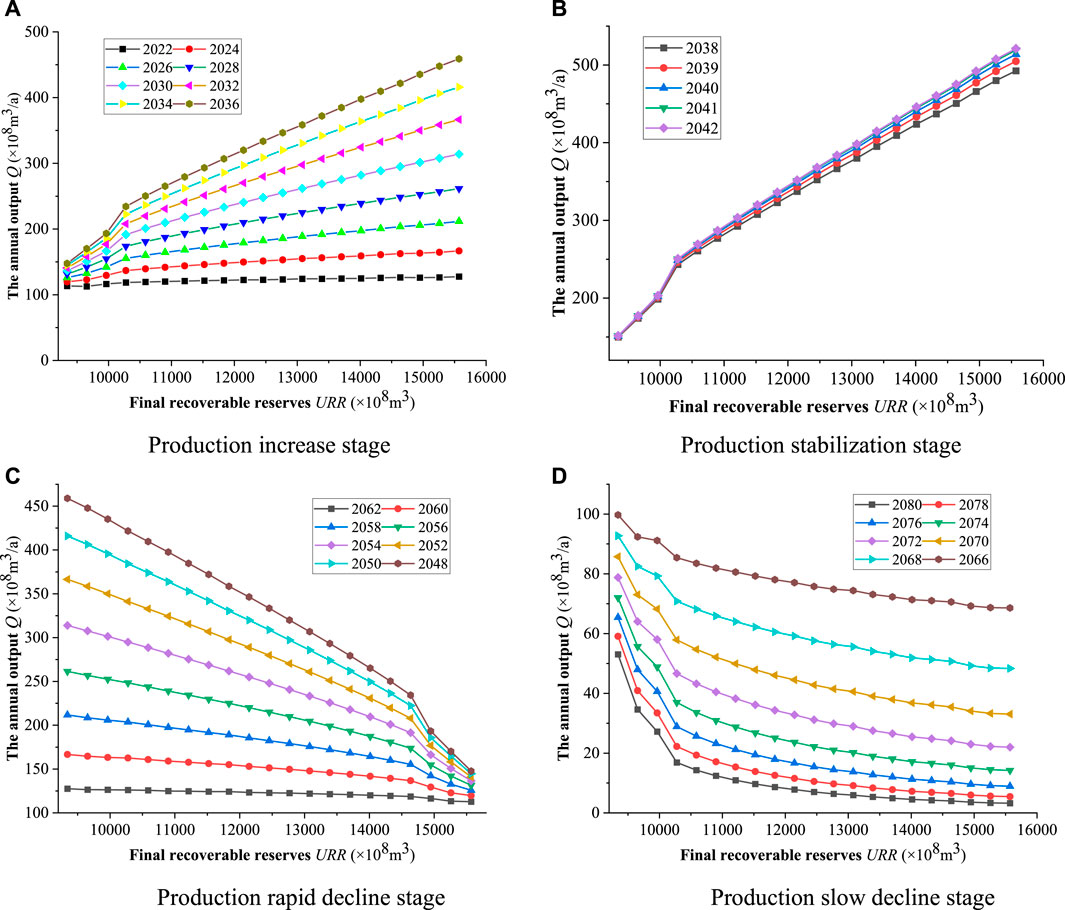
FIGURE 8. Yield prediction results under different URR. (A) Production increase stage. (B) Production stabilization stage. (C) Production rapid decline stage. (D) Production slow decline stage.

Taking the result diagram of the production increase stage of Figure 8A as an example, the meaning of the URR-yield prediction result diagram is described. Figure 8A is a dot line diagram, with lines of different colors representing the production of different years. The details of the dot chart are as follows:

The lines in different colors represent the trend of production in different years with the increase of URR. The abscissa in the figure is the URR corresponding to the production, and the ordinate represents the annual output. For example, the brown line in Figure 8A corresponds to the yield year of 2036. The abscissa of the upper right of the brown line in the figure is 15,570 and the ordinate of the top is 458.99. The coordinate of the point on the top right of the adjacent yellow line is 402.78, and the difference of the ordinate of the two points can be calculated as 56.21. That is, when $URR=15570\times {10}^8{m}^3$, the annual production of 2036 $Q=458.99\times {10}^8{m}^3$, and the difference between it and 2034 $Q=402.78\times {10}^8{m}^3$ is $\mathrm{\Delta }Q=56.21\times {10}^8{m}^3$.

Monte Carlo method can calculate the different production realization probability of four production growth stages each year. In the mathematical model of probabilistic simulation based on Gauss yield calculation equation of Formula (10), URR is the main independent variable affecting production. The year 2030 is taken as an example to introduce the probability calculation process. Since the value of URR is uniformly extracted, the uniformly distributed URR value is directly randomly extracted for multiple times. Set the extraction times of URR as 100,000 times and extract each URR value to obtain the corresponding $Q_m$ and $t_m$ values from Figure 7B respectively, and put them into Formula (10) together with t=2030 to obtain the output Q in 2030.

After 100,000 times of production calculation, the distribution probability of annual production value Q is calculated, and the corresponding cumulative probability is obtained through a cumulative way, which is the realization probability of production. Due to the uniform distribution of URR, the accuracy of production probability statistics can be guaranteed. Figure 9 shows the production realization probability results of representative years in four stages. Table 3 shows the calculation results of realization probability of annual output at different stages.

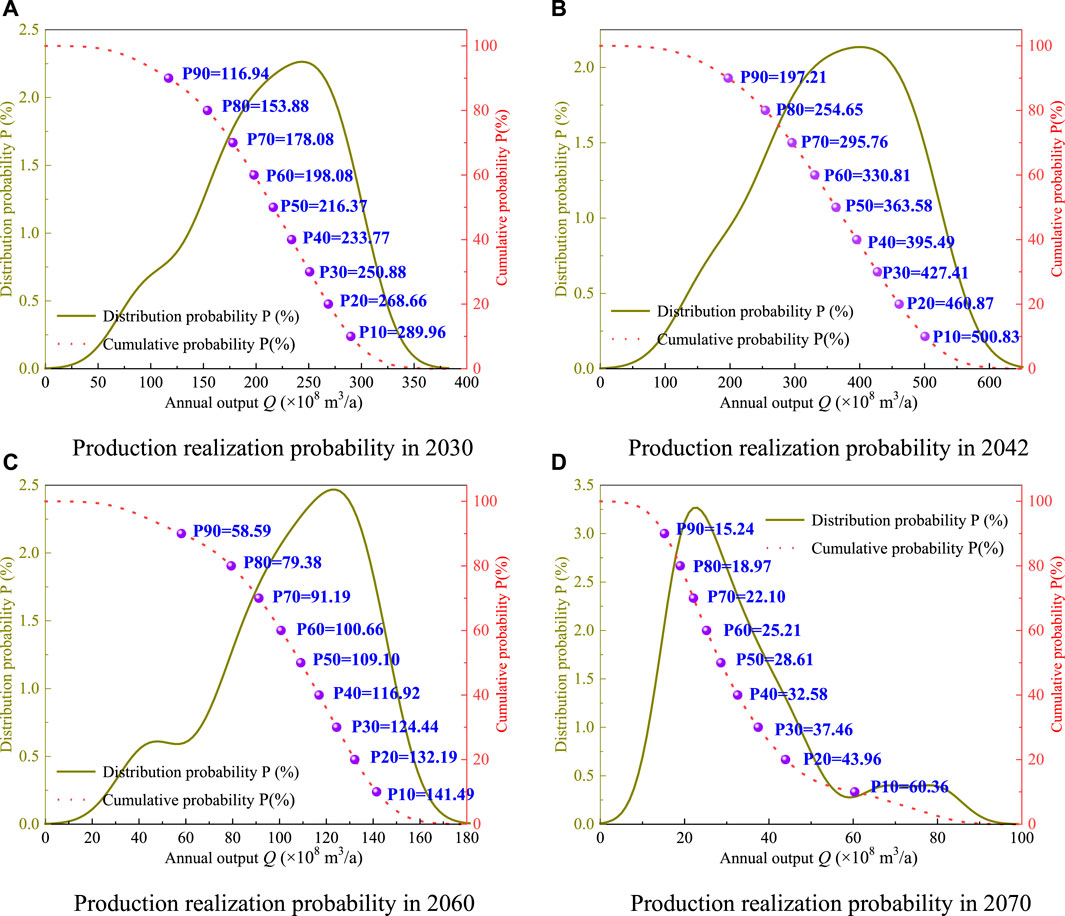
FIGURE 9. Yield realization probability calculation in different years. (A) Production realization probability in 2030. (B) Production realization probability in 2042. (C) Production realization probability in 2060. (D) Production realization probability in 2070.

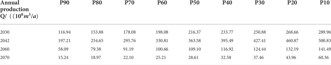
TABLE 3. Production realization probability calculation results of different stage years.

The cumulative probability and realization probability both represent the possibility of output reaching the corresponding scale. In 2060, “$\text{P}80=79.38\times {10}^8{m}^3/\text{a}$” means that the probability of production reaching $79.38\times {10}^8{m}^3/\text{a}$ is 80%. In this paper, the risk of shale gas production in different probability intervals is calculated and the risk is quantified. Where, the production of P80 is guaranteed, the production of P50 is the average yield, and the production of P20 is ideal. The probability of different shale gas development targets can be obtained from the production simulation results, which provides important reference and guidance for the formulation and feasibility analysis of shale gas exploration and development plans.

Production risk level evaluation based on matrix analysis

By introducing a risk matrix (Figure 3), quantitative risk research and risk grade evaluation are conducted on shale gas production. According to the probability calculation method in Section 4.2, the probability of production distribution in each year of the four stages is obtained and the realization probability curve is drawn. According to the distribution probability curve, the mean value μ and standard deviation s of annual output are calculated, and then substituted into Formula (13), the dispersion degree c of annual output was obtained.

In the stage of increasing production and slowly decreasing production, 5% <C ≤10%. At this time, p > 80% corresponds to grade II risk, 20% ≤ p <5 0% corresponds to grade III risk, and p < 20% corresponds to grade IV risk.

10% < C ≤ 25% in stable production stage and rapid production decline stage. In this case, p>50% corresponds to grade III risk, while p ≤ 50% corresponds to grade IV risk.

In view of the value range of C in different stages, the yield realization probability curves of different years in the four stages are superimposed with the areas of risk matrix to obtain the annual yield target risk levels in different stages (Figure 10).

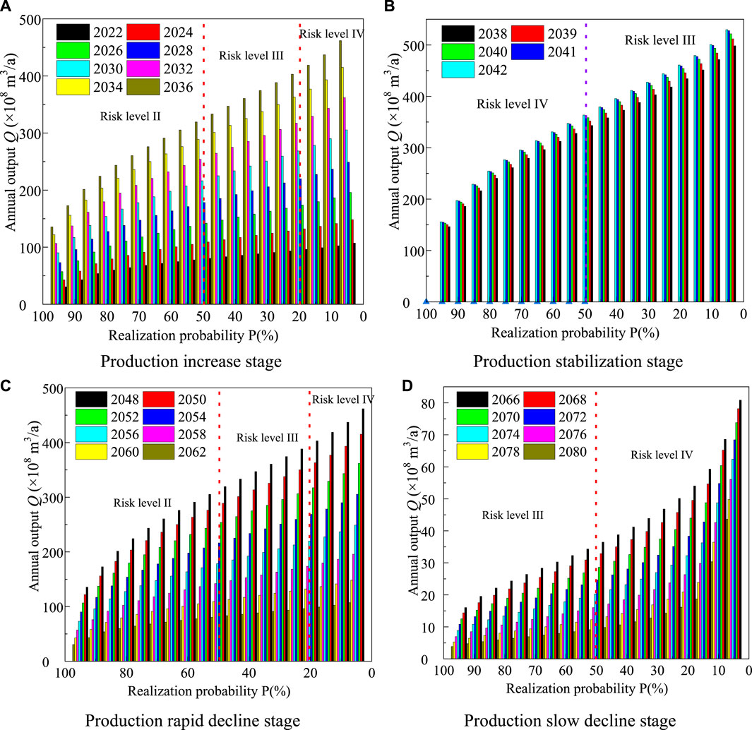
FIGURE 10. Production risk rating evaluation. (A) Production increase stage. (B) Production stabilization stage. (C) Production rapid decline stage. (D) Production slow decline stage.

As can be seen from Figure 10, as the product value increases, the corresponding realization probability decreases gradually, and the risk level of the production realization probability increases accordingly. According to the quantification results of production risk at different stages in Figure 10, the realization probability and risk level of different production in different years can be directly obtained. Because the production risk level indicates that the production target is difficult to achieve, the quantitative study of production risk based on probability calculation and matrix analysis can provide theoretical basis for feasibility analysis of shale gas production target at different time nodes.

Comprehensive evaluation

The quantitative study of shale gas production risk is to analyze the probability distribution of production in each year under the premise of uniform distribution of URR. Based on the evaluation indexes of shale gas production realization probability p and dispersion degree C at different time nodes, the production risk is quantified. By introducing evaluation matrix, risk grade evaluation and target risk analysis of annual production in different production growth stages are carried out.

Due to the low cognition of shale gas exploration and development in Sichuan Basin, the establishment criteria of risk grade evaluation matrix are not fully combined with shale gas exploration and development, so URR is used as the influencing factor of production prediction in this paper. Therefore, with the advance of shale gas exploration and development in the future, the methods of production prediction and risk matrix establishment need to be constantly improved and updated to meet the needs of shale gas exploitation.

Conclusion

In this paper, Hubbert model and Gauss model are used to predict the production growth trend of gas reservoirs. Monte Carlo method is used to simulate the probability of production realization. The conclusions are as follows:

1) when URR is at the same growth rate, Gauss model has a more stable yield growth trend than Hubbert model, and the correlation coefficients of Gauss model are all higher than that of Hubbert model. This means that the production prediction results of the Gauss model have higher accuracy.

2) URR is introduced into Hubbert and Gauss model to forecast shale gas production growth trend. The production growth process can be divided into four stages, and the production growth rate in each stage has obvious difference. Production projections indicate that shale gas production will reach its peak range of $\left(280-460\right)\times {10}^8{m}^3/\text{a}$ in 2042. In 2037–3047, it will be a stable production stage, and the URR recovery will reach 60% at the end of the stable production period.

3) Production risk quantification research based on production prediction results can provide more quantitative basis for shale gas exploration and development. The production growth curve with URR as independent variable was simulated by Monte Carlo, and the production realization probability p of each year with URR as influencing factor was obtained. Combining this index with dispersion degree C, the risk grade evaluation matrix is established. It has promoted the establishment of shale gas production target risk quantification system in Sichuan Basin.

Data availability statement

The raw data supporting the conclusions of this article will be made available by the authors, without undue reservation.

Author contributions

HL and DZ supervised the research and proposed the research direction. GY and YF was responsible for data analysis and paper writing. YC helped in writing the paper. CW helped with some data processing.

Funding

This study was supported by the fund of Petro China South west Oil and Gas Field Company (Grant No. 20200310–06). The authors are grateful for the editor and reviewers’ helpful comments.

Conflict of interest

Authors HL, GY, YF, and YC were employed by PetroChina Southwest Oil & Gas Field Company.

The remaining authors declare that the research was conducted in the absence of any commercial or financial relationships that could be construed as a potential conflict of interest.

Publisher’s note

All claims expressed in this article are solely those of the authors and do not necessarily represent those of their affiliated organizations, or those of the publisher, the editors and the reviewers. Any product that may be evaluated in this article, or claim that may be made by its manufacturer, is not guaranteed or endorsed by the publisher.

References

Chen, J., Guo, L., Zong, G., Nian, J., and Han, H. (2022). Evaluation method of proved recoverable shale gas reserves based on probability statistics: a case study of a shale gas development block in sichuan-chongqing srea [J]. Unconv. oil gas 9 (02), 49–57. doi:10.19901/j.fcgyq.02.07
Deng, B., Lu, Z., Liu, Q., Luo, J., Liu, S., and Peng, Y. (2022). Calculation method of deviation factor and early reserve prediction of shuangyushi ultra-deep HP/HT gas reservoir [J]. Special Oil Gas Reservoirs 29 (01), 73–79.
Du, X., Wu, J., and Liu, M. (2021). Quantitative analysis of the shift of natural gas market gravity center in china [J]. Nat. Gas Technol. Econ. 15 (05), 45–51.
Gutierrez, J. P., Benitez, L. A., Ruiz, E. A., and Erdmann, E. (2016). A sensitivity analysis and a comparison of two simulators performance for the process of natural gas sweetening. J. Nat. Gas Sci. Eng. 31 (11), 800–807. doi:10.1016/j.jngse.2016.04.015
Hu, L. (2022). Research progress on evaluation methods and factors influencing shale brittleness: a review. Energy Rep. 8, 4344–4358. doi:10.1016/j.egyr.2022.03.120
Huang, C., Tian, L., Wang, H., Wang, J., and Jiang, L. (2011). Against conditions generated based prediction model of reservoir single well production networks [J/OL]. Comput. Phys., 1–17.
Li, X., Liang, J., Yuan, H., Du, L., Pei, S., and Luo, Z. (2019) “Technical difficulties and test production technology of high-pressure sulfur gas reservoir in northwestern sichuan basin [C]. ,” in The 31st national convention (2019) on natural gas (02) gas pool development, 81–87. doi:10.26914/Arthurc.nkihy.071913
Li, Z., Liu, J., Ying, L., Hang, W., Hong, H., Ying, D., et al. (2015). Formation and evolution of weiyuan-anyue tensional corrosion trough in sinian system, sichuan basin. Petroleum Explor. Dev. 42 (1), 29–36. doi:10.1016/s1876-3804(15)60003-9
Liang, S., Li, W., Weng, J., Hao, L., Yang, Q., Xia, Y., et al. (2020). Prediction of methanol filling volume and optimization of distribution network of natural gas production pipeline based on BP neural network [J]. Chem. industry oil gas 49 (06), 45–5.
Liu, C., Li, J., Dang, W., Bai, S., and Wang, X. (2020). Wavelet neural network based on genetic algorithm to optimize the short-term gas load forecast [J]. Comput. Syst. Appl. 29 (4), 175–180. doi:10.15888/j.carolcarrollnki.Csa.007338
Lu, C., Song, L., Dong, Y., Chen, G., and Duan, R. (2021)). Oil well production prediction method based on Long term memory neural network model. Petrochem. Ind. Appl. 40 (10), 44–47.
Ma, X., Wang, H., Zhou, S., Shi, Z., and Zhang, L. (2021). Deep shale gas in china: geological characteristics and development strategies. Energy Rep. (7), 1903–1914. doi:10.1016/j.egyr.2021.03.043
Qiao, L., Cui, Y., Gao, H., Chen, L., and Wang, P. (2021). Based on the grey prediction model of gas production rate of coalbed methane reservoir dynamic prediction research [J]. J. Chengde petroleum Coll. 23, 37–41. doi:10.13377/j.carolcarrollnkiJCPC.2021.05.008
Shaolei, W., Huang, X., Li, J., Su, Y., and Pan, L. (2021). Evaluation of final recovery of single shale gas well based on probability method: a case study of infill well in jiaoshiba shale gas field [J]. Petroleum Geol. Exp. 43 (01), 161–168.
Wang, J., Liu, R., Feng, L., and Yu, X. (2020). An improved production prediction model for multi-cycle oil and gas fields [J]. Xinjiang Pet. Geol. 41 (04), 430–434.
Wang, J., Jiang, H., Zhou, Q., Wu, J., and Qin, S. (2016). China's natural gas production and consumption analysis based on the multicycle hubbert model and rolling grey model. Renew. Sustain. Energy Rev. 53 (11), 1149–1167. doi:10.1016/j.rser.2015.09.067
Wang, L. (2022). Exploration and development prospect of shale gas resources in sichuan basin [J]. West. Explor. Eng. 34 (04), 79–80.
Wang, Z., Zhou, X., Li, G., Yu, W., Li, G., Shi, Y., et al. (2020). “Analysis of influencing factors of balance difference of natural gas pipe network in z area and prediction of BP neural network [C],” in The 32nd session of the national convention (2020) on natural gas, 3073–3086. doi:10.26914/Arthurc.nkihy.065218
Xie, J., Guo, G., Tang, Q., Peng, X., Deng, H., and Xu, W. (2021). Key technologies for efficient development of ultra-deep and ancient dolomite karst gas reservoirs: a case study of sinian dengying formation gas reservoirs in anyue gasfield, sichuan basin [J]. Nat. Gas. Ind. 41 (06), 52–59.
Zhang, H., and Rong, C. (2007). Prediction method of oil and gas reserve growth trend and its application in evaluation of offshore oil and gas resources in china [J]. Nat. Gas. Geosci. (05), 684–688.
Zhang, L., Pan, Y., Ren, C., Zhang, H., and Wu, J. (2021). Determination of distribution function of evaluation parameters in gas reservoir reserve calculation by probability method [J]. J. Chongqing Univ. Sci. Technol. Nat. Sci. Ed. 23 (06), 39–44. doi:10.19406/j.cnki.cqkjxyxbzkb.2021.06.009
Zhang, P., Wu, T., Zhong, L., Li, Z., Wang, J., and Ji, L. (2020). BP neural network to predict along the north deep carbonate reservoir stress sensitivity [J]. Petroleum Nat. gas Chem. (5), 622–626. doi:10.13639/j.oDPT.2020.05.016
Zhang, P., Zhang, Y., Zhang, W., and Tian, S. (2021). Numerical simulation of gas production from natural gas hydrate deposits with multi-branch wells: influence of reservoir properties. Energy 9 (6), 1007–1022.
Zhang, S., Wang, Y., and Wang, J. (2021). Risk analysis of universities laboratory behavior based on monte carlo method [J]. J. Exp. Technol. Manag. 38 (9), 279–284. doi:10.16791/j.carolcarrollnkiSJG.2021.09.056
Zhang, Y., Li, P., Li, T., and Li, J. (2019). Study on the peak production of antimony ore in china based on hubbert model [J]. China Min. 28 (08), 66–71.
Zhou, L., Yan, J., Zhao, F., and Zhan, L. (2021). Functional integral method and probability distribution calculation of transfer function in non-gauss random scattering channel model [J]. J. Sichuan Normal Univ. Nat. Sci. Ed. 44 (06), 799–805.
Zhou, Xiangguang, Xunbo, Shuai, and Wu, Bing (2008). Natural gas production forecast based on improved grey model [J]. Nat. Gas. Technol. (04), 70–72+80.
Keywords: shale gas, production prediction, risk quantification, production realization probability, gauss prediction model, Monte Carlo probability method
Citation: Li H, Yu G, Fang Y, Chen Y, Wang C and Zhang D (2022) Gas production prediction and risk quantification of shale gas reservoirs in Sichuan Basin based on Gauss prediction model and Monte Carlo probability method. Front. Earth Sci. 10:977200. doi: 10.3389/feart.2022.977200
Received: 28 June 2022; Accepted: 25 July 2022;
Published: 25 August 2022.
Edited by:
Yihuai Zhang, Imperial College London, United KingdomReviewed by:
Hu Li, Southwest Petroleum University, ChinaQuanzhong Guan, Chengdu University of Technology, China
Copyright © 2022 Li, Yu, Fang, Chen, Wang and Zhang. This is an open-access article distributed under the terms of the Creative Commons Attribution License (CC BY). The use, distribution or reproduction in other forums is permitted, provided the original author(s) and the copyright owner(s) are credited and that the original publication in this journal is cited, in accordance with accepted academic practice. No use, distribution or reproduction is permitted which does not comply with these terms.
*Correspondence: Dongming Zhang, zhangdm@cqu.edu.cn