GSPy: A new toolbox and data standard for Geophysical Datasets

1 Introduction

Accurate management and usage of scientific data is fundamentally dependent on how the data are stored and documented. Community-agreed-upon standards in data formatting and organization are a natural and necessary step in simplifying the transfer and analysis of complex datasets, both within and across disciplines. In the Earth Sciences, many communities of practice have evolved, such as Cooperative Ocean/Atmosphere Research Data Service (COARDS) from the National Oceanic and Atmospheric Administration (NOAA), Common Data Form (CDF) from the National Aeronautics and Space Administration (NASA), or Hierarchical Data Format (HDF) originally developed by the National Center for Supercomputing Applications (NCSA) but currently maintained by The HDF Group (NOAA, 1995; Folk et al., 1999; Yang et al., 2005; NASA, 2019). Notably, the Network Common Data Form (NetCDF) architecture has become the basis for many modern data standards (Rew et al., 2006; Hankin et al., 2010; Unidata, 2021b). Overall, the purpose of a data standard is to control how data and metadata are documented, formatted, and stored such that datasets can be shared, displayed, and operated on with minimal user intervention across platforms and software (Eaton et al., 2020).

Geophysical datasets are widely used in Earth system studies to interrogate subsurface properties and processes. Methods vary considerably, each relying on different physics and are sensitive to different physical properties of Earth materials (e.g., rocks, sediments, and fluids). Geophysical data are commonly acquired using instruments on land, on or beneath water, from airborne platforms, or in boreholes. Broad categories of geophysical methods (e.g., electrical, magnetic, seismic, electromagnetic, radiometric, gravity) have specific measurement modalities (e.g., frequency-domain or time-domain electromagnetics), each of which can have many unique instruments with differing designs and configurations. In addition to the values measured by an instrument’s sensors, a host of other auxiliary information is often needed but contained in separate supplementary files, field notes, or contractor’s reports and not directly attached to the data. The supplementary information includes fundamental positioning information, general survey metadata, as well as details about acquisition parameters or instrument characteristics needed to interpret the measured data. Without this accompanying supplementary information, acquiring meaningful results and interpretations would be a challenge.

Although geophysical datasets have much in common at a basic level—recorded data values, system information, coordinate information, and auxiliary metadata—data formats vary widely by method and by instrument. Probably the most established geophysical formats relate to the Society of Exploration Geophysicists (SEG) digital tape standards used for seismic data, owing to the vast amount of industrial seismic data collection (Northwood et al., 1967; Hagelund and Levin, 2017). Yet, even within data formats that are more widely used in the geophysical community, none meet the criteria of 1) being an open format that allow for publication according to Findability, Accessibility, Interoperability, and Reuse (FAIR) principles in public repositories, 2) attaching important system information and metadata to the data in a single file, and 3) incorporate a file structure that facilitates transferability between open-source computational software, web services, and geospatial systems. The lack of a common open data standard leads to inefficiencies where processing or interpretation software must be customized to read specific formats from different instruments, and data need to be re-formatted before they can be used by software and/or published according to FAIR standards (Wilkinson et al., 2016; Salman et al., 2022).

Similar to seismic acquisitions, airborne geophysical surveys are often acquired by industry for a wide range of government, academic, and private clients. Airborne geophysical surveys are becoming more commonplace, providing cost-effective, high resolution, and multi-scale subsurface imaging not easily obtained with ground-based observations over large areas. As with the field of geophysics overall, there is currently no open community standard that is widely used for sharing and releasing airborne geophysical datasets. Furthermore, airborne datasets entail significant supplementary information on survey design, system and acquisition parameters, and post-processing details that are often included in PDFs or other report documents separate from the digital data, posing a risk to the long-term integrity of the data. The large size and complexity of airborne geophysical data, as well as their broad community value, necessitates accessible tools and standards be developed to keep pace with rising demands and usage.

Efforts have been made in the past to standardize airborne data formats, along with interoperable inversion software for working with airborne electromagnetic (AEM) datasets (Møller et al., 2009; Brodie, 2017). The Australian Society of Exploration Geophysicists (ASEG) established the ASEG-GDF2 (General Data Format Revision 2) data standard (Dampney et al., 1985; Pratt, 2003), an ASCII-based data structure for general point and line data, with particular focus on large airborne geophysical datasets such as magnetic, radiometric, electromagnetic, and gravity. Tabular ASCII data, such as ASEG-GDF2 or CSV, have the advantage of being both human and machine readable for easy usage, but these formats result in larger file sizes compared with binary formats. ASCII formats are also limited in how datasets can be structured, grouped, and documented. For example, the ASEG-GDF2 structure includes general and variable-specific metadata information in separate definition files that accompany the data, but this design requires users to always maintain multiple files. In Denmark, a national, publicly accessible geophysical database (GERDA) hosts numerous types of airborne and ground-based geophysical datasets in a structured relational database (Møller et al., 2009); however, GERDA databases are not easily used or accessed outside of proprietary software. Geosoft databases are also an industry standard for delivery and storage of airborne geophysical tabular datasets. Their binary format has advantages in data compression and file size, and Geosoft databases are supported by sophisticated software such as Oasis Montaj (Seequent Ltd. https://www.seequent.com/products-solutions/) for processing, analysis, and visualization. However, use of this software requires a commercial subscription, and the binary Geosoft databases do not meet open standards for publication. Lastly, gridded data and products often accompany airborne datasets and can be provided in many binary and ASCII raster formats (e.g., TIF/GeoTIFF, ARC/INFO, GXF, Geosoft GRD, Surfer GRD, etc.), each compatible with one or more of the commonly used software tools. However, some tools are open while others are proprietary and require paid subscription.

Here, we present a data standard using the NetCDF file format that provides a structure for storing geophysical data, metadata, and survey information in a single file. The proposed geophysical standard (GS) balances the need to require information for certain datatypes be stored in a well-defined structure, while also allowing for flexibility with optional information. In addition to recorded data, we use the hierarchical group structure within the NetCDF file to store multiple related datasets or products together. For example, separate groups might contain raw data, processed data, and physical property models determined through inversion or other analyses. Storing digital data along with associated coordinate and system information in a single self-describing open file structure with well-established standards can greatly improve the interoperability, transferability, and impact of geophysical datasets. The underlying HDF data structure is computationally advantageous when compared to human-readable ASCII files (Yang et al., 2005; Rew et al., 2006).

Along with the new GS data convention, we developed a Python package (GSPy) as a community tool which facilitates use of the NetCDF file structure. A basic function of GSPy is conversion, either reading original input files into our proposed data structure and creating the standardized NetCDF file or converting content from the standard structure into a different format needed to work with specific software or for cooperator and end-user needs. Beyond this basic input-output functionality, GSPy can also be incorporated into processing and visualization workflows utilizing the GS structure. Though GSPy is not required to work with the GS data model—any tools capable of interacting with a NetCDF file can be used—we developed GSPy as a building block to make the process of transforming datasets into the GS structure easy and straightforward to maximize their usability.

In this paper, we define the proposed data standard and provide an overview of the GSPy software structure and functionality. Our focus in the initial stage of development of the GS model and associated GSPy tools has been on airborne geophysical data due to their immediate need for an open-source community standard, while also keeping in mind flexibility in design to allow future accommodation of other types of geophysical data in the same model. We use an existing airborne geophysical dataset from Wisconsin as a case study to exemplify the GS convention and demonstrate usage of the GSPy package (Minsley et al., 2022). Finally, we discuss the scalability, limitations, and opportunities provided by a NetCDF-based community geophysics data standard.

2 Methods

Our goal with the GS data model and GSPy software tool is to assimilate data from a variety of file formats, geometries, and geophysical methods into a common and open data structure that can be broadly shared and utilized (Figure 1). The GS data model provides a common, open, and standardized framework for geophysical datasets, which is disconnected and independent from the original source formatting.

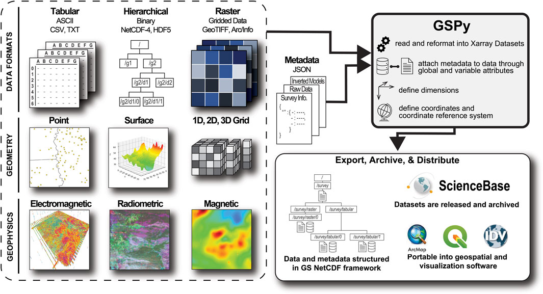
FIGURE 1. Conceptual diagram of GSPy workflow. Data from a variety of formats and types are read into GSPy, along with required metadata files. Through the GSPy software, data are converted into a standardized NetCDF file containing the dataset and metadata appropriate for archiving and sharing.

In airborne surveys, data from one or more geophysical sensors (e.g., electromagnetic, magnetic, radiometric, gravity) are acquired along relatively linear flight lines covering large areas. Data are stored at a regular sampling interval typically in tabular format, and published in ASCII files such as CSV or ASEG-GDF2 (e.g., Ley-Cooper et al., 2019; Drenth and Brown, 2020; Shah, 2020; Minsley et al., 2021). Data from multiple sensors acquired at the same time (e.g., electromagnetic and magnetic) are often combined in a singular tabular dataset at the same sample interval. Two-dimensional rasterized data, typically gridded maps of measured values (e.g., flight altitude or powerline monitor) and/or multi-dimensional interpreted products (e.g., resistivity depth slices or residual magnetic intensity), are often included with contractor-delivered datasets or as publicly archived products. In addition to geophysical sensor data, each measurement also includes important auxiliary information needed for quality control, processing, interpretation, and visualization. Auxiliary metadata includes information such as the position and attitude of the aircraft and geophysical sensors during acquisition, flight line numbers and fiducials, timestamps, noise channels (e.g., powerline monitoring channel for AEM data), and processed or corrected data channels. The GS convention, through GSPy, integrates airborne geophysical data and auxiliary metadata from these various input formats and geometries into a standardized NetCDF file that can be publicly released and shared through data repositories like ScienceBase (https://www.sciencebase.gov), and is portable to common geospatial and visualization software (Figure 1).

2.1 Geophysical data standard

To support efficient metadata documentation, combined storage of related datasets, and transferability to multiple software tools and web services, the GS data model is founded within the NetCDF file format. NetCDF was established in 1989 by the University Corporation for Atmospheric Research (UCAR)’s Unidata program (Rew and Davis, 1990), who continue to provide development and support for newer NetCDF versions and related software (Rew et al., 2006; Unidata, 2021b). The latest version, NetCDF-4 is built on the HDF5 storage layer and format (Rew et al., 2006). As modern datasets are becoming larger and more complex, e.g., studies are more often data-rich and/or employ “big data” approaches (Vermeesch and Garzanti, 2015; Shelestov et al., 2017; Reichstein et al., 2019; Li and Choi, 2021) the appeal of NetCDF is growing. Organizations such as NASA, NOAA, National Snow and Ice Data Center (NSIDC), and National Center for Atmospheric Research (NCAR) have adopted NetCDF as one of their preferred formats (Ramapriyan and Leonard, 2021, see complete list of users at https://www.unidata.ucar.edu/software/netcdf/usage.html). We have chosen to follow the same path, recognizing the many advantages provided by the NetCDF format:

• Self-describing: Metadata are directly attached to datasets. This architecture eliminates any risk of critical metadata becoming separated from the data, which can severely reduce dataset usability. This structure is especially important in geophysical datasets, where auxiliary system information such as transmitter waveforms, time gates, or transmitter-receiver coil orientations are essential for accurate analysis and interpretation of the data.

• Space-saving: The binary format has a smaller file size compared to ASCII files. Extra packing and compression options can further reduce file sizes.

• Accessible: Subsets of large datasets can be accessed directly without needing to read in the full dataset, thereby minimizing memory requirements.

• Portable: Files are platform-independent, meaning datasets are represented uniformly across different computer operating systems.

• Hierarchical: Multiple datasets can be stored in a single file following a tiered group organization. This structure provides a clean and efficient mechanism for archiving and sharing related datasets in a single file, such as raw versus processed data, in addition to inverted models and any products derived from those models.

• Scalable: Files can be read from and written to using large-scale distributed memory machines, allowing fast access at massive computational scales.

The GS design builds on existing conventions in other Earth science disciplines. Specifically, we adapt and extend the Climate and Forecast (CF) Metadata Conventions (hereafter, the CF conventions; Eaton et al., 2020) to satisfy the needs of geophysical datasets. The CF conventions ensure datasets conform to a minimum standard of description, with common fields and elements, and guarantee data values can be accurately located in time and space (Eaton et al., 2020). The CF conventions originated as an extension of the COARDS NetCDF convention from NOAA (NOAA, 1995), and are Unidata’s recommended standard of choice. The GS convention follows the rules and guidelines of the CF standard, with additional constraints in grouping datasets and metadata while also allowing for nuances inherent to geophysical datasets. Specific details on GS-specific metadata requirements are outlined in the GSPy documentation pages (Foks et al., 2022).

2.1.1 GS group structure

The hierarchical nature of NetCDF allows for groups of multiple self-described datasets within a single file, where each dataset can have differing structure or dimensions and can be accessed separately using a defined path, similar to a file system directory path (e.g., /group1/group2). The GS data model contains three fundamental categories for grouping data and metadata (Figure 2). General metadata for the dataset(s) as a whole are contained within the Survey group. Every file is required to have a Survey group which sits at the root of the hierarchical group structure and contains all data subgroups (Figure 2B). Data are then categorized by the nature and geometry of the values. Unstructured data, such as scattered points or lists of values, are contained within the Tabular group. Structured data, i.e., gridded data, are contained within the Raster group. Having two separate data groups is meant to ease import/export of datasets with minimal manipulation or alteration, thereby ensuring transparency and accountability in cataloging processing steps as well as improving accessibility in data handling. For example, a Raster dataset can immediately be exported to a GeoTIFF file, whereas a Tabular dataset would require modification such as interpolation onto a regular grid. When there are multiple datasets attached to a single group, we separate them with a simple integer index (e.g., /survey/tabular/0 and /survey/tabular/1, in the case where two tabular entries are attached).

1) Survey: This group contains general metadata about the dataset, or collection of related datasets, within the NetCDF file. General information about where the data was collected, acquisition start and end dates, who collected the data, any clients or contractors involved, system specifications, equipment details, and so on are contained within data variables of the Survey group. Information included in the Survey group is often provided or recorded separately from the data, such as in contractor PDF reports or field notes. Attaching this digital metadata preserves important survey details and facilitates processing and analysis, for example, by including instrument parameters needed for visualization or geophysical inversion. Users are allowed to add as much or little information to the Survey data variables as they choose. However, following the CF convention, we require a set of global attributes [e.g., title, institution, source, history, references, see section 2.6.2. of Eaton et al. (2020)]. In the GS standard, we add an additional “content” key that provides a brief summary of what datasets are included in the file and their locations, e.g., “raw data at /survey/tabular/0”. Secondly, a “coordinate_information” variable is required within Survey and should contain all relevant information about the coordinate reference system. More details on handling coordinate reference systems are described in section 2.1.2.

2) Tabular: Data that is organized in a tabular format, such as a CSV file with discrete locations along rows and measurement values along columns, are read and categorized into a Tabular group. In the case of airborne geophysics this would include data collected at discrete points along flight lines, inverted physical property models determined from measured data, or any other type of scattered point data.

3) Raster: Data that is structured into predefined grids are categorized into the Raster group. Generally, this includes two-dimensional (2D) and three-dimensional (3D) gridded data, such as interpolated geophysical models or surfaces.

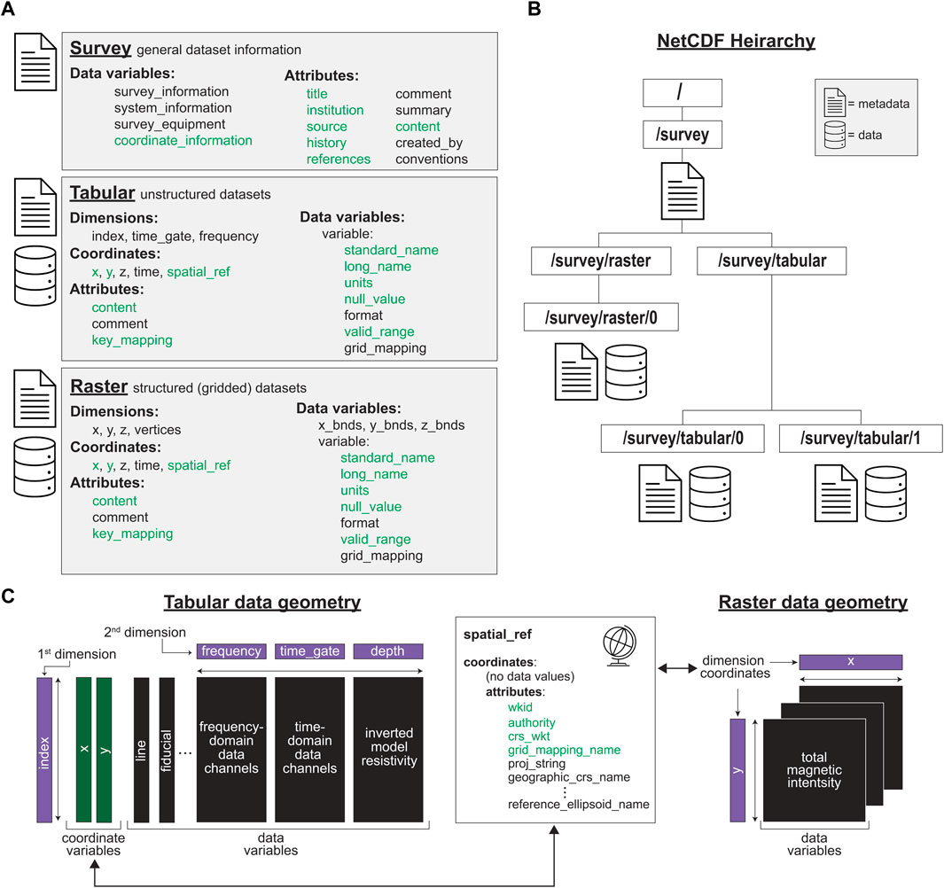
FIGURE 2. GS data convention. (A) Datasets are structured into three fundamental group types based on content and data geometry. The Survey group contains general metadata about the dataset. Unstructured datasets, such as from CSV or TXT files, form Tabular groups, whereas structured (gridded) datasets are categorized under the Raster group. Metadata is attached to all groups, with various required attributes (green text) that expands on the CF-1.8 convention. (B) Groups follow a strict hierarchy in the NetCDF file, with a single Survey group at the top to which all data groups are attached. Datasets are indexed within their respective group type. (C) Tabular and Raster data groups must contain clearly defined dimensions, such as index or x, y, z, as well as coordinate variables. Raster groups are distinct in that dimensions are also coordinates, whereas Tabular datasets are assigned spatial coordinates that align with the index dimension. Lastly, the coordinate variable “spatial_ref” is required for all data groups, which expands on the “coordinate_information” variable required in the Survey metadata.

Data groups are located a level below the Survey group in the NetCDF file and have access to the same global metadata (Figure 2B). The hierarchical group structure allows for multiple related datasets to be stored and shared together, such as raw data, processed data, inverted models, and any products derived from those models. This structure also inherently provides an audit trail for users, thereby encouraging transparency and dataset integrity. It is best practice to provide meaningful variable and dimension names and follow established conventions (e.g., CF) or community norms whenever possible. A small set of global attributes are required for all data groups, as well as required variable attributes, and a defined “spatial_ref” variable containing the coordinate system information (Figure 2A).

The relationship between dimensions, coordinates, and data values differs between Tabular and Raster groups (Figure 2C). For Tabular datasets, data variables are more often one-dimensional (1D), such as columns in a CSV, which are by default given an “index” dimension. For 2D or 3D variables, the second or third dimensions are defined and attached to the dataset, such as measurement time gates for time-domain AEM data channels, or frequencies for frequency-domain data channels. All data groups require spatial coordinate variables, standardized as “x” and “y”. In the case of Tabular data, the coordinate variables match the size of the 1D index dimension and are sourced from corresponding input data variables, e.g., the longitude and latitude of data points, through the “key_mapping” attributes. In contrast, Raster datasets are gridded such that the dimensions of the data are also the coordinates (Figure 2C). A Raster group may contain multiple variables (e.g., total magnetic intensity and residual magnetic field) if all variables within the dataset share the same dimensions, otherwise separate Raster groups are encouraged (e.g., /survey/raster/0 and /survey/raster/1).

2.1.2 Coordinate reference systems

All datasets are required to have a defined coordinate reference system to maintain accurate representation of data values for both visualization and analysis purposes. Information about the coordinate system, such as a Well-known ID (WKID; Esri, 2016) and corresponding authority (e.g., EPSG), if it is geographic or projected, horizontal and vertical datums, and so on are stored within the Survey group’s required “coordinate_information” variable. Any Tabular or Raster datasets attached to the Survey must have a matching variable “spatial_ref” and adhere to the same coordinate reference system. Following CF conventions (see section 5.6 of Eaton et al. (2020)), the “spatial_ref” coordinate variable must have the attribute “grid_mapping_name” which ties to a corresponding “grid_mapping” attribute within the data variables. Additionally, the “x” and “y” coordinate variables require certain attributes, such as “GeoX” and “GeoY” for “_CoordinateAxisType” which connects to a related key in the “spatial_ref” variable. If the coordinate system is a projection, then the “standard_name” keys for “x” and “y” should be “projection_x_coordinate” and “projection_y_coordinate”. These details ensure that datasets are portable and accurately represented within geospatial systems (Eaton et al., 2020; Esri, 2022).

2.1.3 NcML

The last piece of the GS convention is the NetCDF eXtensible Markup Language (XML), NcML, metadata file, which is an XML representation of the metadata and group structure within the NetCDF file. NcML files are commonly used to allow simple updates or corrections to the metadata contained within NetCDF files (Nativi et al., 2005). For example, the Thematic Real-time Environmental Distributed Data Services (THREDDS) data server (TDS) employs NcML to define new NetCDF files, or augment and correct existing files hosted on their web service (Caron et al., 2006; Unidata, 2021c). NcML files also serve as a quick means for users to gain an overview of NetCDF file contents without needing to access the binary files. The NcML is not required to understand the data or metadata, but are an optional component that we recommend including when sharing or archiving GS NetCDF files.

2.2 GSPy v0.1.0

To implement this new GS data convention, we developed an open-source Python package, GSPy, which provides a basic toolkit to build, interface with, and export standardized geophysical datasets. GSPy utilizes the extensive Xarray Python package to assemble the GS groups and read/write the NetCDF files (Hoyer and Hamman, 2017). Xarray’s architecture consists of DataArrays and Datasets. An Xarray DataArray is a labeled, multi-dimensional array containing 1) “data”: an N-dimensional array of data values, 2) “coords”: a dictionary container of the data coordinates, 3) “dims”: the dimensions for each axis of the data array, and 4) “attrs”: an attribute dictionary of key metadata (e.g., units, null values, descriptions) (Hoyer and Hamman, 2017). An Xarray Dataset is a collection of DataArrays, and similarly has the components of “dims” and “coords” which reflect those of the DataArrays (categorized as “data_vars” in the Dataset) and “attrs” for global metadata attributes that describe the collection. In the GS structure, each Tabular and Raster data group, as well as the Survey group, are individual Xarray Datasets. The data variables (DataArrays) within the Survey group’s Dataset are unique in that they contain no data values, only variable attributes of Survey metadata information.

The GSPy package can be found at https://doi.org/10.5066/P9XNQVGQ, and requires Python version 3.5 or later (Foks et al., 2022). The software is platform independent (operates on both Windows and Unix operating systems) and has been released under the CC-0 license as per U.S. Geological Survey (USGS) software release policy. In this initial version, GSPy primarily serves as a data conversion tool, with functionality to interface with multiple input data formats and output to a GS-structured NetCDF file. Metadata is currently documented and input to GSPy through user-prepared JSON files.

2.2.1 Classes

GSPy contains Survey and Data classes, and the Data class is extended to the Tabular and Raster classes allowing for specific handling of those data types. The code requires a Survey object be instantiated as the first step to building a GS dataset (Figure 3A). A JSON metadata file (Figure 3B) is required to initialize the Survey object, where dictionaries such as “system_information,” “survey_equipment,” and “coordinate_information,” for example, become data-less DataArray variables within the Survey’s Dataset, consisting primarily of metadata within the variable attributes. The required dictionary “dataset_attrs” populates the Dataset attributes, most of which follow the CF convention required inputs.

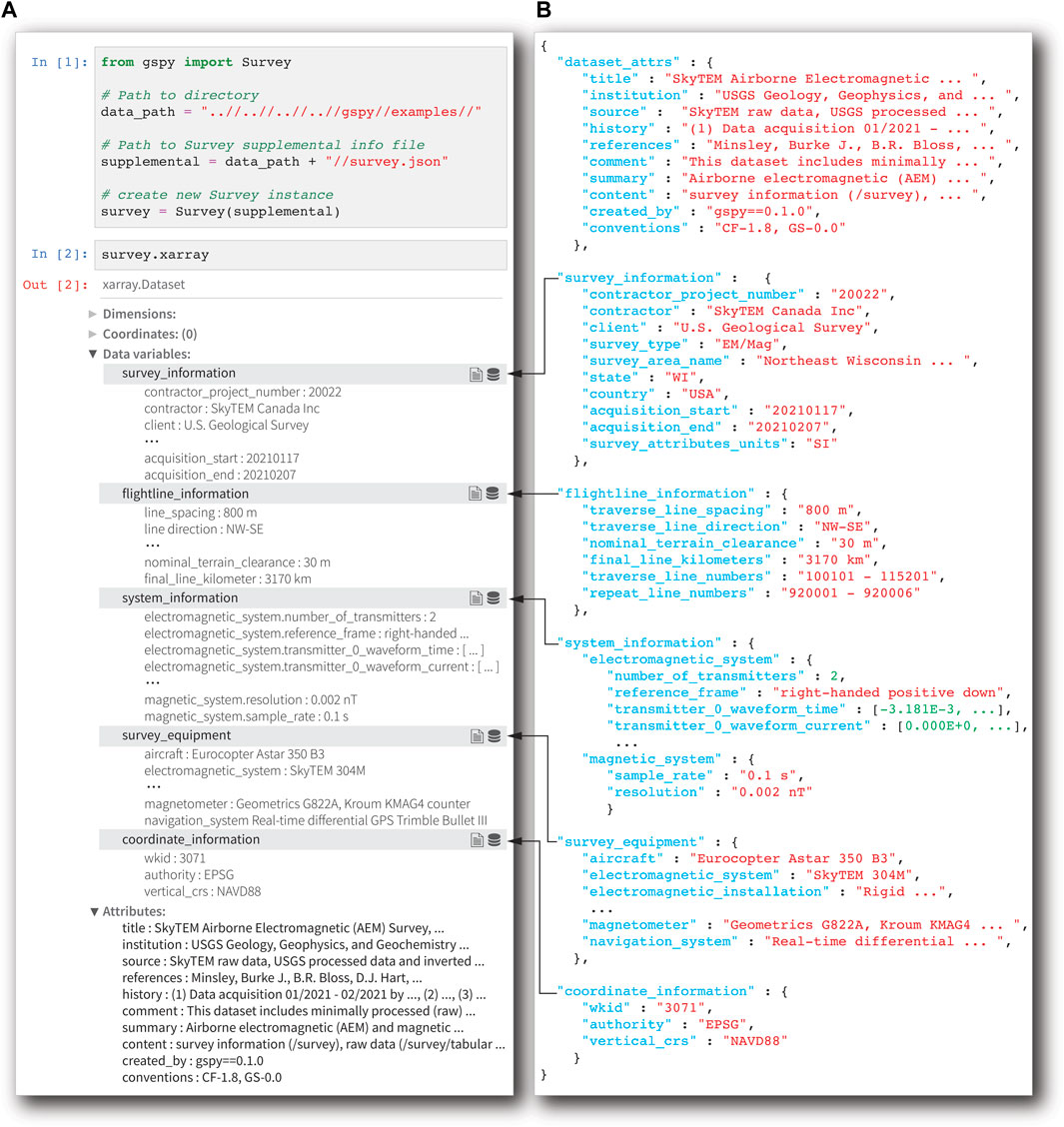
FIGURE 3. Starting a GS dataset with the GSPy package. (A) A GS dataset is always initialized with an instance of the Survey class. General metadata about the project and survey are read from a JSON file (B) and formatted into an Xarray Dataset attached to the Survey class object. The “dataset_attrs” dictionary contains required fields that populate the general attributes of the Xarray Dataset, while all other dictionaries become DataArray variables (black arrows).

Each data assemblage, typically contained within a single tabular text file or a collection of related raster files, are attached to the established Survey object as the appropriate Data class using the “add_tabular” or “add_raster” methods of the Survey (Figure 4A, Figure 5A). Each instance of “add_tabular” and “add_raster” appends a new class object, Tabular or Raster, respectively, to the Survey with an incremented index for each location once written to disk, e.g., /survey/tabular/0, /survey/tabular/1, and /survey/tabular/2. The code is ignorant of any meaningful descriptions of data type, e.g., raw data vs. inverted models, and instead handles data purely based on the input format type and geometry. Therefore, it is up to the user to ensure the metadata—we recommend the “content” attribute field—provide sufficient description of what each Dataset within a Survey contains.

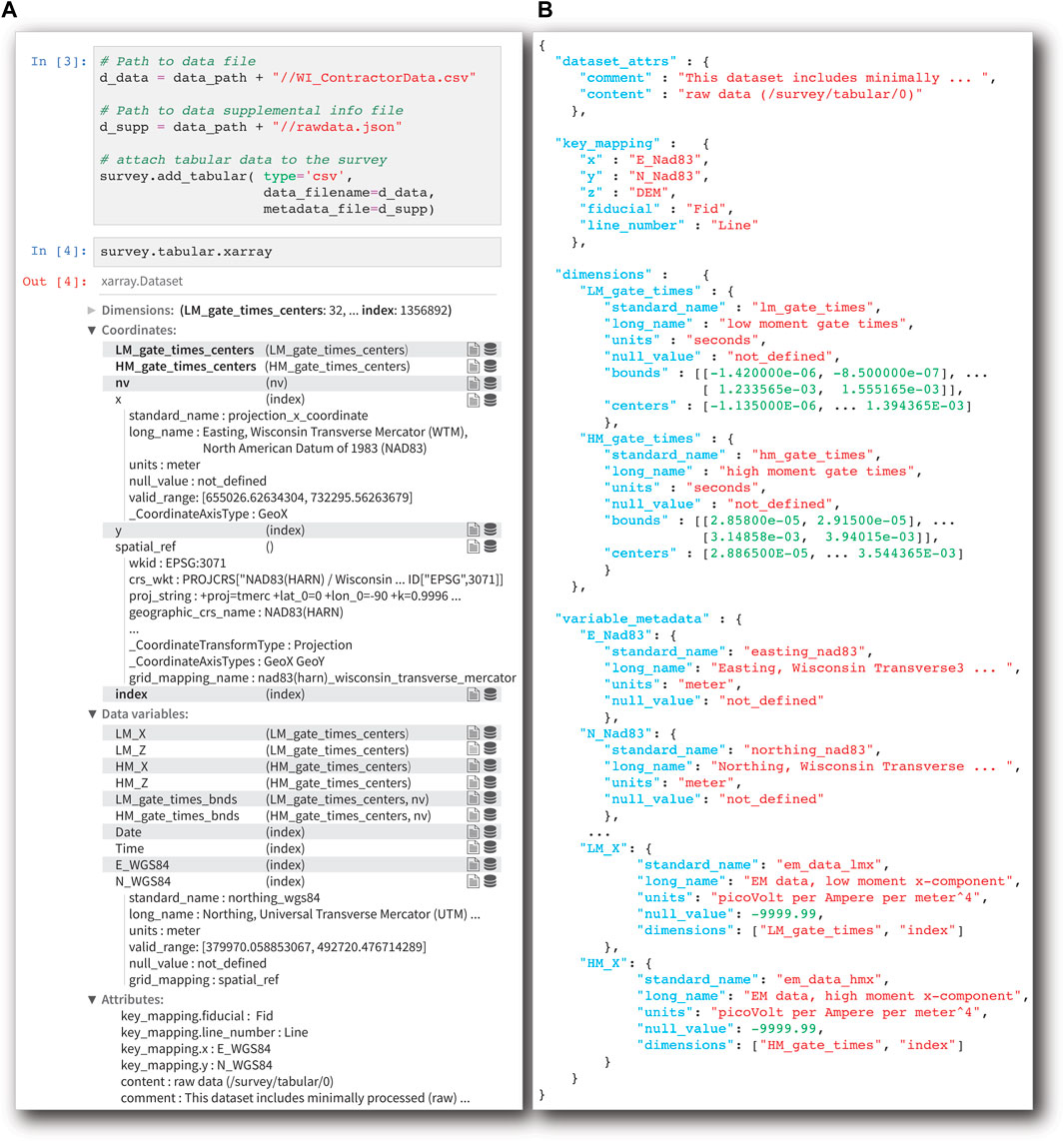
FIGURE 4. Attaching a Tabular group to a Survey. (A) The “add_tabular” method is used to add a Tabular Dataset to Survey. (B) The Dataset attributes, coordinate “key_mapping,” variable-specific metadata, and any second-dimension variables are passed through a required JSON file when attaching the Tabular group.

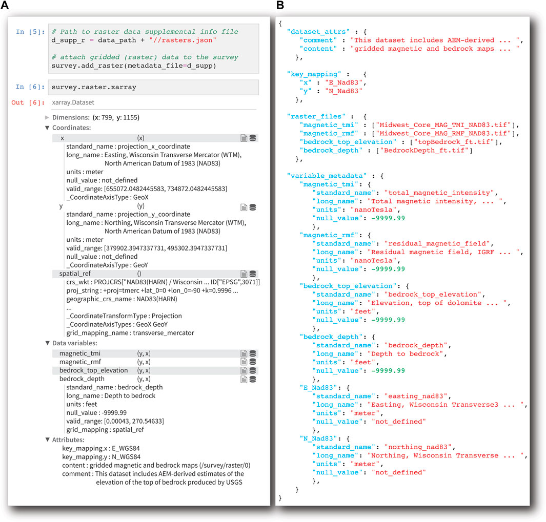
FIGURE 5. Attaching a Raster group to a Survey. (A) The “add_raster” method is used to add a Raster Dataset to Survey. (B) As with Tabular groups, the Dataset attributes, coordinate “key_mapping”, and variable-specific metadata are passed through a required JSON file. The Raster class allows for a one-to-one mapping of GeoTIFF files to DataArray variables within the Dataset, or multiple files can be stacked into a single variable. The “raster_files” dictionary maps the desired variables to its input file(s).

GSPy version 0.1.0 supports CSV and ASEG-GDF2 text file formats for Tabular groups. For CSV files, a “variable_metadata” dictionary needs to be passed through the JSON file (Figure 4B). In contrast, ASEG-GDF2 files allow for variable attributes to be populated from the structured ASEG definition (.dfn) metadata file (Pratt, 2003). The “variable_metadata” dictionary can be optionally included for ASEG files to add or overwrite metadata values. For both input file types, GSPy executes one-to-one mapping of columns into DataArrays by default. Variables that comprise multiple columns are handled in one of two ways. First, if the columns contain an incrementor following the variable name formatted as [0], [1], …. [N] for N number of columns—a common format for geophysical datasets—then the columns are concatenated in order and labeled by the root column name. For example, a time-domain AEM variable that appears as “EMX_HPRG [0]”, “EMX_HPRG [1]”, “EMX_HPRG [2]” etc. within the contractor-provided data file would be combined into a 2D DataArray variable, “EMX_HPRG”, within the GSPy Dataset. In this example, the dimensions of the “EMX_HPRG” variable would be “index” and “gate_times.” The “gate_times” dimension values and metadata are also defined through the JSON file in the “dimensions” dictionary (Figure 4B). For Tabular groups, users also have the option to provide bounds on dimensions, when appropriate, such as the start and end times for each time gate. We follow the CF conventions’ approach to bounding variables, such that a rank 1 dimension of length N will have bounds of shape (N, 2), where each value along the first axis has 2 vertices corresponding to its bounds (Figure 4).

The second approach to multi-dimensional column variables is to pass a “raw_data_columns” key within the “variable_metadata” dictionary of the JSON for the desired output variable name, where the values of “raw_data_columns” points to the original column names in the data file in the order they should be concatenated. For example, a frequency-domain AEM variable for in-phase filtered data can often appear in the raw data file with unique columns named by frequency, such as “cpi400_filt”, “cpi1800_filt”, etc. A sorted list of these data columns should be passed through the metadata of a new variable, such as “ip_filtered,” which would have the dimensions “index” and “frequency.” As before, the “frequency” dimension would be defined and described through a “dimensions” dictionary. Coordinates for Tabular data are defined through the “key_mapping” dictionary of the JSON. As stated previously, Tabular variables have coordinates of dimension “index” and the “key_mapping” allows GSPy to create the coordinate variables based on named input variables, e.g., {“x”: “Longitude”, “y”: “Latitude”}.

GSPy v0.1.0 supports GeoTIFF files as the primary input/output format for Raster groups. In contrast to Tabular groups, variables are added either as 2D variables from single GeoTIFF files (1 file = 1 DataArray) or 3D variables by stacking multiple files along a named dimension (e.g., individual depth slices). In the JSON metadata file, the “raster_files” dictionary maps each DataArray variable to a file or list of files. As before, a “variable_metadata” dictionary is needed to complete the attributes of each variable. The dimensions of the data are by default the coordinates defined by the input file, thus no “dimensions” dictionary is needed. The “key_mapping” dictionary is still needed for Raster datasets to update the metadata of the dimension coordinates (“x” and “y”). We use the Rioxarray module (http://github.com/corteva/rioxarray) to go between GeoTIFF files and Xarray DataArrays. Upon reading in a GeoTIFF file, GSPy compares the input coordinate reference system with that of the Survey. If the input reference system does not match, the DataArray is reprojected using Rioxarray. Future versions can follow the same procedures for other standard raster data file formats.

For all data types regardless of geometry (Tabular and Raster), the JSON metadata file is required to contain a “dataset_attrs” dictionary, which populates the attributes of the Dataset. Since data groups are contained within the Survey group of the NetCDF file, the globally required attributes of the Survey apply to all data groups, per CF conventions (Eaton et al., 2020). Therefore, the attributes of data groups only require the “content” key and any “key_mapping”, with additional keys such as “comment” optionally included at user-discretion. Lastly, the coordinate reference system of the Survey is used to create the “spatial_ref” coordinate variable to accompany each Dataset, thereby requiring all groups under a Survey to have matching coordinate systems. Either a well-known identification (WKID) number and associated authority, e.g., EPSG:4326, or a coordinate reference system well-known text (CRS_WKT) string are needed to then generate the complete “spatial_ref” variable using the GDAL and Pyproj packages (GDAL/OGR contributors, 2022; https://github.com/pyproj4/pyproj). We follow CF conventions and ArcGIS guidelines (e.g., Esri, 2022) to ensure proper transferability of datasets into common geospatial and NetCDF-supported software.

2.2.2 Class properties and methods

GSPy provides many helpful properties and methods for working with datasets. Here we highlight some essential functions, and refer readers to the GSPy documentation pages for a complete description of all classes, methods, and functionality, along with code examples (Foks et al., 2022).

First, all classes share the property of “xarray” to return the GS-formatted Xarray Dataset (Figures 3, 4, 5A). The “read_metadatafile” method is common to each class and attaches the full dictionary read from the provided JSON file to the property “json_metadata”. If a metadata file does not get passed or is missing required dictionaries, the “write_metadata_template” method is called to generate a template file that users can then edit. This function is useful for large CSV datasets with many variables, as it will generate a “variable_metadata” dictionary based on the column names. All attributes are given “not_defined” values that users can then update.

Once all groups have been attached to a Survey, the “write_netcdf” and “write_ncml” methods will write the GS-structured NetCDF file and accompanying NcML file, respectively (Figure 6). The data classes, Tabular and Raster, also contain “write_netcdf” functions to export groups in separate files; however, we recommend always using the Survey class “write_netcdf” function to adhere to the standard with all groups written to a single file. The Tabular and Raster classes also contain export methods such as “to_csv” and “to_tif”, respectively. Lastly, some simple plotting methods are provided for both Raster and Tabular classes using Xarray’s scatter and pcolor functions (Figure 6).

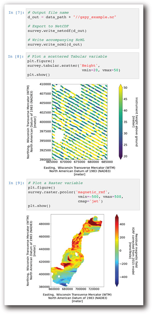
FIGURE 6. Writing and plotting examples. Once all groups have been attached to a Survey, the “write_netcdf” and “write_ncml” methods will write the GS NetCDF and NcML files, respectively. GSPy also provides methods to generate scatter and pcolor plots for variables.

3 Results

To demonstrate the proposed GS convention and the functionality provided by GSPy, we converted a recently acquired airborne geophysical dataset into the new standard through GSPy workflows. This dataset provides the opportunity to showcase examples of diverse input data formats (CSV and GeoTIFF) and geometries (Tabular and Raster) within the proposed GS architecture. In January and February 2021, the U.S. Geological Survey oversaw collection of 3,170 line kilometers of AEM and magnetic data over northeast Wisconsin through collaboration with the Wisconsin Department of Agriculture, Trade, and Consumer Protection (DATCP) and Wisconsin Geological and Natural History Survey (WGNHS) (Minsley et al., 2022). The primary purpose of this effort was to improve understanding of the depth to bedrock across the study area. The airborne data were acquired by SkyTEM Canada Inc. with the SkyTEM 304M time-domain helicopter-borne electromagnetic system together with a Geometrics G822A cesium vapor magnetometer.

Input data consisted of 1) a CSV file (3.17 GB) of contractor-provided raw AEM and magnetic data along with auxiliary flight data; 2) a CSV file (123.9 MB) of processed AEM data; 3) a CSV file (145.3 MB) of inverted resistivity models; 4) a CSV file (4.4 MB) of AEM-derived point estimates of the elevation of the top of bedrock; and 5) four GeoTIFF files containing gridded magnetic data (total magnetic intensity: 7.4 MB, residual magnetic field: 7.4 MB), AEM-derived gridded depth to the top of bedrock (3.7 MB) and top of bedrock elevation (3.7 MB). We created JSON files for the Survey group, pulling critical information on the flightlines, system parameters, and equipment from the contractor-provided report (Figure 3B). Each CSV file was added as a separate Tabular group with an individual JSON metadata file (e.g., Figure 4B). The four GeoTIFF files were added as variables within a single Raster group with an accompanying JSON file (Figure 5B).

With the GSPy workflow, and proper documentation in the JSON files, all datasets were assembled under the Survey group with complete dataset- and variable-specific metadata, mapping of dimensions and coordinates, and standardized coordinate reference systems variables. We then used GSPy methods to export the combined datasets into a single NetCDF file and generate the NcML metadata file. Figure 7 shows a simplified version of the NcML file, with essential elements represented. Both NetCDF and NcML files were publicly released in ScienceBase (Minsley et al., 2022). The size of the final GS NetCDF file was 1.93 GB, corresponding to a file size reduction of 44% relative to the original input files without utilizing further compression. The complete file and its contents were accurately imported into common NetCDF software such as Unidata’s Integrated Data Viewer (IDV) (Unidata, 2021a). Raster variables from the full GS NetCDF file were accurately imported into Quantum Geographic Information System (QGIS), with correct placement, coordinate reference system, and null value representation. ArcMap was unable to import the full NetCDF file comprising multiple groups, but datasets exported to individual files, at the root group position, were accurately imported. Notably, both scattered Tabular data and gridded Raster data were successfully viewed in ArcMap, but we were unable to view scattered data in QGIS.

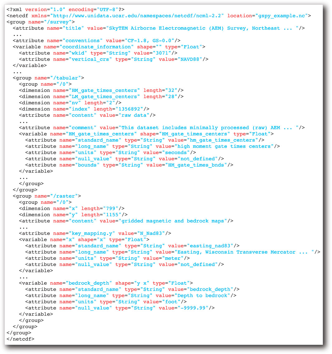
FIGURE 7. Example NcML file. Due to space constraints, only essential elements are shown here for example representations. Gaps in variable and attribute lists are noted by ellipses.

4 Discussion

The GS data convention improves the accessibility and functionality of geophysical datasets by providing much-needed standards for the storage of both data and metadata built on the established NetCDF open data structure and existing CF conventions. By building on the NetCDF CF conventions, the GS model has several advantageous characteristics summarized earlier: it is self-describing, space-saving, accessible, portable, scalable, and hierarchical. Most importantly, the GS model allows multiple types of geophysical data and incremental data processing steps to be stored together in a single self-described file with all variable-specific and general survey metadata attached. Our support for unstructured point data (tabular) within the NetCDF is particularly novel, as both historical and modern implementations of the NetCDF format have dominantly been for gridded (raster) datasets (e.g., Hankin et al., 2010; Eaton et al., 2020; Morim et al., 2020). These characteristics are important for both the long-term accessibility and interoperability of geophysical datasets. While our focus here is on airborne geophysical surveys, this data model can be readily extended to other survey data that can be described in tabular or raster formats.

Application of the GSPy workflow and GS data model to a real airborne geophysical dataset resulted in several successful outcomes and insights. First, what began as several disconnected, undocumented, and uniquely formatted data files became a single NetCDF file with related, self-described datasets clearly categorized and standardized. This improved the shareability and usability of the data, as every variable and dataset group were fully documented and easily accessed within the single file. Second, the NetCDF file, and its accompanying NcML file, was all that was needed to be archived for public release. This resulted in a significantly simplified data release process, i.e., file preparation, metadata documentation, and the review process were all streamlined compared to a traditional release of the original data files and incomplete metadata documentation. Lastly, the standardized datasets within the NetCDF file were accurately viewed and represented within common NetCDF and GIS software, signifying the broad transferability and interoperability of the GS format.

We recognize the aforementioned advantages of using the NetCDF file structure also comes with some challenges. Accessing information in binary NetCDF files may be a barrier for users not familiar with this format, especially compared with ASCII-based file formats. The accompanying GSPy software tools include methods for exporting to common tabular or raster formats if those are needed for specific end-users. Additionally, raising awareness about common GIS or other software tools that can read NetCDF files, along with their current limitations, will be important. Preparing the JSON metadata files can be time consuming, but once prepared executing the GSPy workflow is straightforward and efficient. Furthermore, datasets being published in an open repository would need much of the same metadata information, prepared here in JSON input files, to instead be produced in XML or other online metadata records. Thus, we recognize that documentation of metadata can be a tedious endeavour but a necessary one nevertheless. While accessibility and ease-of-use need to be continually improved upon, such as changing to a slightly more user-friendly metadata input format like Yet Another Markup Language (YAML), for example, the additional complexity of the GS convention is outweighed by its broader advantages discussed above. Upfront time costs with the GSPy workflow will likely balance out with time savings during archival, as well as improve overall dataset usability and impact.

The first version of GSPy has focused on an implementation of the GS data model for airborne geophysical data; however, we have developed the software, data classes, and functions with the intention of being generalized and adaptable to all types of geophysical methods. We plan to layer new functionality for ground-based and airborne geophysical data alike in future versions, such as method-specific converters for ground resistivity data and models or seismic timeseries. A guiding principle is to build a strong foundation for the data standard and software tools that can be readily extended to other datatypes without changing the basic structure. Any number or type of classes can be attached as groups within the hierarchical NetCDF file structure, always falling under a general metadata Survey group. Most geophysical datasets and related products can be described by the generic Tabular or Raster classes, and additional classes can be developed as needs are identified. By developing GSPy as an open-source package, our goal is to enable a broad community of users to improve its functionality and capabilities.

New GSPy functionality is planned for future versions to simplify import and export workflows, such as automatically recognizing different datatypes and routing to customized methods that handle different datatype requirements. Support for other data formats and software interfaces is also planned, for example leveraging existing packages such as gxpy (https://github.com/GeosoftInc/gxpy) to directly import data from commonly used binary Geosoft databases and sciencebasepy (https://github.com/usgs/sciencebasepy) to automate the publication process to the USGS ScienceBase repository. Accessibility can also be broadened by including documentation and links in future versions for common software programs that can read GS-structured NetCDF files.

Additional worked examples of other airborne geophysical datasets and data types are needed to continue refining the structural details of how data and metadata are imported to and stored in the GS data model. For example, identifying and revising required versus recommended versus optional attributes and variables, defining generic and adaptable structures for storing Survey metadata information, and standardizing JSON templates for various data types will improve the overall usability of the data standard. Future GSPy functionality can also be added to aid in data processing and visualization—eventually with GSPy serving as a central platform for importing datasets, processing, exploring, reformatting, interfacing with various inversion software, and exporting in a standardized format for public release. Additionally, we plan to explore the use of web-based tools such as the THREDDS Data Server (Caron et al., 2006; Unidata, 2021c) for accessing and subsetting content from GS-structured files stored in online repositories, without needing to download entire datasets.

If adopted as a common standard for geophysical datasets, further efficiency could be realized by having instruments or contractor-delivered datasets directly create GS-structured files, or at least the information needed to readily create them. Likewise, processing, visualization, and inversion software tools could directly read files in the GS convention without having to export other specialized input formats. For example, the study presented in this paper required multiple file format conversion steps throughout the workflow: contractor-provided databases and PDF reports, processed data, inverted geophysical models, and bedrock elevation picks were all exported from proprietary software tools into CSV and JSON formats to prepare them for publication in open formats. Significant improvements in workflow efficiency and interoperability can be achieved by using the GS convention as a link that connects instrument-recorded data and metadata to processing, visualization, and interpretation tools as well as archival-ready data structures.

5 Conclusion

The field of geophysics encompasses diverse and complex data formats that can vary between methods, techniques, and from one collection to another. Inconsistencies in data and metadata documentation reduce the longevity and impact of geophysical datasets. To address the pressing need for a community-supported geophysical data standard, we have developed the GS convention, based on the NetCDF file format and CF metadata conventions. The GS convention meets the goals we set out to achieve in a geophysical data standard:

• The format is open source meeting the requirements of FAIR data publication standards.

• The file format allows for multiple related and self-described datasets to be grouped together under a clear and standardized hierarchical structure.

• Dataset- and variable-specific attributes join important auxiliary information and metadata directly to the digital data, ensuring dataset integrity, longevity, and interoperability.

• Data dimensions and coordinates are clearly defined, along with a well-defined coordinate reference system for accurate visualization and representation.

• The format is transferable between open-source computational software, web services, and geospatial systems.

The accompanying open-source Python package, GSPy, facilitates efficient data conversion between common data formats (e.g., CSV, ASEG-GDF2, GeoTIFF), proper metadata documentation through JSON supporting files, and export of GS NetCDF files. We demonstrated the GS structure and GSPy workflow using an example airborne geophysical dataset from Wisconsin. The single resulting GS NetCDF file was significantly reduced in size compared to the multiple ASCII-text and GeoTIFF input files. Furthermore, metadata that was previously distributed throughout a contractor-provided PDF report was cleanly incorporated and appropriately attached to specific dataset groups and variables. Aside from a few limitations identified, such as the group structure in ArcMap or scattered data in QGIS, the GS-formatted file and/or individual data groups were successfully loaded and accurately represented in geospatial software.

Adoption of the GS standard for airborne geophysical data fills a particular need for an open-source, community-wide standard that ensures accurate archival of critical metadata jointly with digital datasets. Moreover, establishment of a NetCDF-based open data standard for a broad range of geophysical survey types can help to greatly improve how these complex datasets are shared and utilized, making the data more accessible to a broader science community and the public. File formats and functionality supported by GSPy v0.1.0 is limited; however, by developing the standard and package as open source, we aim to leverage the broad geophysical community to contribute to the continued development of robust data standard requirements and tools to facilitate their use.

Data availability statement

The dataset used in this work to demonstrate the GSPy code implementation and GS convention can be found on the U.S. Geological Survey’s data repository, ScienceBase, located at https://doi.org/10.5066/P93SY9LI. The GSPy code repository is located at https://doi.org/10.5066/P9XNQVGQ.

Author contributions

BM led the conceptualization and overall design of the geophysical data standard. NF and SJ developed the GSPy software and worked with BM on designing the GS structure and its practical implementation. SJ led the writing effort for this article, which was contributed to by all authors.

Funding

This work was jointly supported by the USGS Water Availability and Use Science Program and the USGS Mineral Resources Program.

Acknowledgments

The authors thank JR Rigby (USGS) for supporting this effort. We also thank Bennett Hoogenboom (USGS) for helpful comments and review of the software, as well as Jade Crosbie (USGS), Andrew Leaf (USGS), and Urminder Singh (Iowa State University) for their helpful reviews of the manuscript. Any use of trade, firm, or product names is for descriptive purposes only and does not imply endorsement by the U.S. Government.

Conflict of interest

Author NF is employed by Apogee Engineering LLC as a contractor to the U.S. Geological Survey.

The remaining authors declare that the research was conducted in the absence of any commercial or financial relationships that could be construed as a potential conflict of interest.

Publisher’s note

All claims expressed in this article are solely those of the authors and do not necessarily represent those of their affiliated organizations, or those of the publisher, the editors and the reviewers. Any product that may be evaluated in this article, or claim that may be made by its manufacturer, is not guaranteed or endorsed by the publisher.

References

Brodie, R. (2017). ga-aem: Modelling and inversion of airborne electromagnetic (AEM) data in 1D. Geosci. Aust. Available at: https://github.com/GeoscienceAustralia/ga-aem.
Caron, J., Davis, E., Ho, Y., and Kambic, R. (2006). “UNIDATA’s THREDDS data server,” in 22nd International Conference on Interactive Information Processing Systems for Meteorology, Oceanography, and Hydrology.
Dampney, C. N. G., Pilkington, G., and Pratt, D. A. (1985). ASEG-GDF: The ASEG standard for digital transfer of geophysical data. Explor. Geophys. 16, 123–138. doi:10.1071/EG985123
Drenth, B. J., and Brown, P. J. (2020). Airborne magnetic survey, iron mountain-chatham region, central upper peninsula, Michigan, 2018. Reston, VA: U.S. Geol. Surv. data release. doi:10.5066/P91EF3CI
Eaton, B., Gregory, J., Drach, B., Taylor, K., Hankin, S., Blower, J., et al. (2020). NetCDF Climate and Forecast (CF) metadata conventions version 1.8. Available at: https://cfconventions.org/Data/cf-conventions/cf-conventions-1.8/cf-conventions.html.
Esri (2016). Faq: What does “authority: EPSG” mean in an ArcGIS desktop .prj file? Esri Tech. Support. Available at: https://support.esri.com/en/technical-article/000011199 (Accessed May 23, 2022).
Esri (2022). Spatial reference for netCDF data. ArcGIS Deskt. - ArcMap 10.8. Available at: https://desktop.arcgis.com/en/arcmap/latest/manage-data/netcdf/spatial-reference-for-netcdf-data.htm (Accessed May 19, 2022).
Foks, N. L., James, S. R., and Minsley, B. J. (2022). GSPy: Geophysical data standard in Python. U.S. Geol. Surv. softw. release. doi:10.5066/P9XNQVGQ
Folk, M., McGrath, R. E., and Yeager, N. (1999). Hdf: An update and future directions. in IEEE 1999 International Geoscience and Remote Sensing Symposium. IGARSS’99 (Cat. No. 99CH36293), 273–275.
GDAL/OGR contributors (2022). {GDAL/OGR} geospatial data abstraction software library. doi:10.5281/zenodo.5884351
Hagelund, R., and Levin, S. A. (2017). SEG-Y revision 2.0 data exchange format. Soc. Explor. Geophys. Houst.
Hankin, S. C., Blower, J. D., Carval, T., Casey, K. S., Donlon, C., Lauret, O., et al. (2010). “NetCDF-CF-OPeNDAP: Standards for ocean data interoperability and object lessons for community data standards processes,” in Proceedings of OceanObs’09: Sustained Ocean Observations and Information for Society, Venice, Italy, 21-25 September 2009. Editors HallJ, D. E. Harrison, and D. Stammer (Venice, Italy: ESA Publication WPP-306). doi:10.5270/OceanObs09.cwp.41Vol. 2
Hoyer, S., and Hamman, J. (2017). xarray: ND labeled arrays and datasets in Python. J. Open Res. Softw. 5, 10. doi:10.5334/jors.148
Ley-Cooper, Y., Roach, I., and Brodie, R. C. (2019). Geological insights of Northern Australia’s AusAEM airborne EM survey. ASEG Ext. Abstr., 1–4. doi:10.1080/22020586.2019.12073170
Li, G., and Choi, Y. (2021). HPC cluster-based user-defined data integration platform for deep learning in geoscience applications. Comput. Geosci. 155, 104868. doi:10.1016/j.cageo.2021.104868
Minsley, B. J., Bloss, B. R., Hart, D. J., Fitzpatrick, W., Muldoon, M. A., Stewart, E. K., et al. (2022). Airborne electromagnetic and magnetic survey data, northeast Wisconsin (ver. 1.1, June 2022). Reston, VA: U.S. Geol. Surv. data release. doi:10.5066/P93SY9LI
Minsley, B. J., James, S. R., Bedrosian, P. A., Pace, M. D., Hoogenboom, B. E., and Burton, B. L. (2021). Airborne electromagnetic, magnetic, and radiometric survey of the Mississippi Alluvial Plain. Reston, VA: U.S. Geol. Surv. data release. doi:10.5066/P9E44CTQ
Møller, I., Søndergaard, V. H., Jørgensen, F., Auken, E., and Christiansen, A. V. (2009). Integrated management and utilization of hydrogeophysical data on a national scale. Near Surf. Geophys. 7, 647–659. doi:10.3997/1873-0604.2009031
Morim, J., Trenham, C., Hemer, M., Wang, X. L., Mori, N., Casas-Prat, M., et al. (2020). A global ensemble of ocean wave climate projections from CMIP5-driven models. Sci. Data 7, 105. doi:10.1038/s41597-020-0446-2
NASA (2019). CDF user’s guide, version 3.8.0. Sp. Phys. Data facil. NASA/goddard sp. Flight cent., 1–164. Available at: https://spdf.gsfc.nasa.gov/pub/software/cdf/doc/cdf380/cdf380ug.pdf.
Nativi, S., Caron, J., Davis, E., and Domenico, B. (2005). Design and implementation of netCDF markup language (NcML) and its GML-based extension (NcML-GML). Comput. Geosci. 31, 1104–1118. doi:10.1016/j.cageo.2004.12.006
NOAA (1995). Cooperative Ocean/Atmosphere research data service. Natl. Ocean. Atmos. Adm. Available at: https://ferret.pmel.noaa.gov/Ferret/documentation/coards-netcdf-conventions.
Northwood, E. J., Weisinger, R. C., and Bradlei, J. J. (1967). Recommended standards for digital tape formats. Geophysics 32, 1073–1084. doi:10.1190/1.32060004.1
Pratt, D. A. (2003). ASEG-GDF2 A standard for point located data exchange. Aust. Soc. Explor. Geophys. 4, 1–34. Available at: https://www.aseg.org.au/sites/default/files/pdf/ASEG-GDF2-REV4.pdf.
Ramapriyan, H. K., and Leonard, P. J. T. (2021). Data product development guide (DPDG) for data producers version 1.1. NASA Earth Sci. Data Inf. Syst. Stand. Off. doi:10.5067/DOC/ESO/RFC-041VERSION1
Reichstein, M., Camps-Valls, G., Stevens, B., Jung, M., Denzler, J., Carvalhais, N., et al. (2019). Deep learning and process understanding for data-driven Earth system science. Nature 566, 195–204. doi:10.1038/s41586-019-0912-1
Rew, R., and Davis, G. (1990). NetCDF: An interface for scientific data access. IEEE Comput. Graph. Appl. 10, 76–82. doi:10.1109/38.56302
Rew, R., Hartnett, E., and Caron, J. (2006). “NetCDF-4: Software implementing an enhanced data model for the geosciences,” in 22nd International Conference on Interactive Information Processing Systems for Meteorology, Oceanograph, and Hydrology.
Salman, M., Slater, L., Briggs, M., and Li, L. (2022). Near-surface geophysics perspectives on integrated, coordinated, open, networked (ICON) science. Earth Space Sci. 9, e2021EA002140. doi:10.1029/2021EA002140
Shah, A. K. (2020). Airborne magnetic and radiometric survey, Charleston, South Carolina and surrounds, 2019. Reston, VA: U.S. Geol. Surv. data release. doi:10.5066/P9EWQ08L
Shelestov, A., Lavreniuk, M., Kussul, N., Novikov, A., and Skakun, S. (2017). Exploring google earth engine platform for big data processing: Classification of multi-temporal satellite imagery for crop mapping. Front. Earth Sci. 5. doi:10.3389/feart.2017.00017
Unidata (2021a). Integrated data viewer (IDV) version 6.0. BoulderCent: CO UCAR/Unidata Progr. doi:10.5065/D6RN35XM
Unidata (2021b). Network common data form (netCDF). BoulderCent: CO UCAR/Unidata Progr. version 4.8.1. doi:10.5065/D6H70CW6
Unidata (2021c). THREDDS data server (TDS) version 5.3. BoulderCent: CO UCAR/Unidata Progr. doi:10.5065/D6N014KG
Vermeesch, P., and Garzanti, E. (2015). Making geological sense of ‘Big Data’ in sedimentary provenance analysis. Chem. Geol. 409, 20–27. doi:10.1016/j.chemgeo.2015.05.004
Wilkinson, M. D., Dumontier, M., Aalbersberg, Ij. J., Appleton, G., Axton, M., Baak, A., et al. (2016). The FAIR Guiding Principles for scientific data management and stewardship. Sci. data 3, 160018. doi:10.1038/sdata.2016.18
Keywords: data standards, NetCDF, open-source software, geophysics, airborne geophysics
Citation: James SR, Foks NL and Minsley BJ (2022) GSPy: A new toolbox and data standard for Geophysical Datasets. Front. Earth Sci. 10:907614. doi: 10.3389/feart.2022.907614
Received: 30 March 2022; Accepted: 11 July 2022;
Published: 23 August 2022.
Edited by:
Michael Fienen, United States Geological Survey, United StatesReviewed by:
Andrew Leaf, United States Geological Survey, United StatesUrminder Singh, Iowa State University, United States
Copyright © 2022 James, Foks and Minsley. This is an open-access article distributed under the terms of the Creative Commons Attribution License (CC BY). The use, distribution or reproduction in other forums is permitted, provided the original author(s) and the copyright owner(s) are credited and that the original publication in this journal is cited, in accordance with accepted academic practice. No use, distribution or reproduction is permitted which does not comply with these terms.
*Correspondence: Stephanie R. James, sjames@usgs.gov