Evolution Characteristics and Mechanism of the Load/Unload Response Ratio Based on Strain Observation Before the Jiuzhaigou M_S7.0 Earthquake

1 Introduction

On 8 August 2017, an Ms7.0 Jiuzhaigou earthquake (JZGEQ) occurred in Sichuan province in China (103.82°E, 33.2°N) with a depth of ∼9 km. The result of the global centroid moment tensor (GCMT, see Data and Resources) solution (Ekström et al., 2012) shows that the rupture of JZGEQ is mainly dominated by strike-slip motion, and the rupture also contains ∼10% of thrusting non-double-couple (NDCP) components (Sun et al., 2018). The strike of JZGEQ is 165° to the SSE direction, and the dip angle is 85°. JZGEQ occurred on the hidden fault named Shuzheng fault in the north of the Huya fault, and the post-seismic geological survey shows that there is no surface rupture around the epicenter (Nie et al., 2018). The northeastern margin of the Tibet Plateau is the junction of the Qaidam block, the Bayan Har block, and the Yangtze block (Figure 1A). Therefore, the rupture processes of the Huya fault are highly complex (Sun et al., 2018; Liu et al., 2019), and several major seismic events have occurred in the history.

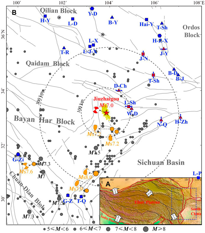
FIGURE 1. (A) Location diagram of the study area. Red lines: primary block boundary; Black lines: secondary block boundary; Black arrow: movement direction of the plate; Blue dotted rectangle: location of Figure 1B. (B) Regional tectonic setting, historical earthquake, and strain observation stations distribution around JZGEQ. Gray dots: seismic events above Ms5 in the study area since 1900s; Orange dots: Seismic events above Ms7 since 1970s; Focal mechanism: epicenter events above Ms7 since 1970s (cite from GCMT); Gray circle: epicentral distance of 100 and 300 km; Triangle: cave strainmeter station; Square: four-gauge borehole strainmeter station; Hexagonal: volumetric borehole strainmeter station; Red icon: stations in Figure 2; Blue arrow: direction of the strain observation; L-Sh: Liang-Shui station; W-D: Wu-Du station; D-Ch: Dang-Chang station; N-Q: Ning-Qiang station; H-Zh: Han-Zhong station; T-Sh: Tian-Shui station; J-N: Jing-Ning station; B-J: Bao-Ji station; B-D: Ba-Du station; J-Y: Jing-Yuan station; L-J-X: Liu-Jia-Xia station; L-X: Lin-Xia station; T-R: Tong-Ren station; H-Z-X: Hai-Zi-Xia station; T-Sh: Tan-Shan station; Hai-Y: Hai-Yuan station; B-Y: Bai-Yin station; Y-D: Yong-Deng station; L-D: Le-Du station; H-Y: Huang-Yuan station; G-Zi: Gan-Zi station; G-Z: Gu-Zan station; T-Q: Tian-Quan station; L-P: Liang-Ping station.

In the northeastern margin of the Tibet Plateau, a large number of strain observation instruments have been deployed by the China Earthquake Administration (Figure 1B). As the most intuitive observation equipment to explore stress change in the crust, aforementioned equipment provides a large number of practical and reliable data for the complete record of stress adjustment in the region before and after JZGEQ. However, it is quite difficult to identify the damage process of rock media prior to the occurrence of the earthquake directly by strain observation. Domestic and foreign scholars tried to use GNSS to study the large-scale stress adjustment before and after strong earthquakes above M7, which further promoted the understanding of seismic phenomena and physical processes (Wang et al., 2001; Shen et al., 2009; Wang and Shen, 2020). However, due to the limitation of GNSS observation time, regional stress adjustment results cannot be obtained in real time. Wang et al. (2020) tried to solve the time problem by using the continuous observation of GNSS, who recorded the pre-seismic anomalies related to the Lushan Ms7.0 earthquake. The strain transition characteristics within a period of less than two and half years can be used as an observable and identifiable precursor to forecast an impending earthquake. However, the ambiguous anomalies and the uncertain time scales still make it difficult to predict the rupture degree of rocks in the crust, and we still need to explore the physics mechanism of earthquake preparation.

In this study, we find that the load/unload response ratio (LURR) method based on strain observation may be used to solve the physical processes related to earthquake preparation. The LURR notion is proposed by Yin (1987) by calculating the Benioff strain of small earthquakes during the loading phase and unloading phase. Then, the method is continuously applied and developed by different scholars (Zhang et al., 2004; Yu et al., 2015; Liu and Yin, 2018), and the calculating data are developed from the seismic catalog to the groundwater level. Previous studies show that the LURR time series can reflect the change of stress state in the heterogeneous brittle system (Yin et al., 1995; Yin et al., 2000). According to the mechanical experiment results of rock, when it is in the elastic stage, the responses during the loading and unloading phases are almost the same. As a result, LURR during this period is about 1.0 (Supplementary Figure S1). However, when the force of the system exceeds the elastic limit of the rock, the responses during the loading and unloading phases will not be equal, and LURR during this period will exceed 1.0. This difference in the responses reflects the damage of a loaded material, and many results also prove that the LURR time series have the phenomenon of abnormal enhancement before large earthquakes (Yu et al., 2006; Yu and Zhu, 2010; Liu and Yin, 2018). Therefore, the LURR value may be served as a useful parameter to evaluate rock rupture and provide a basis for the future seismic risks in this region. However, most of the studies use the seismic catalog or groundwater level as input data, as the most intuitive way to monitor stress change, few scholars use the strain data directly for the LURR calculation. As a result, by using the LURR method based on strain observation, we try to identify the response difference of earth tide during the loading phase and unloading phase, so as to determine the stress state of the source medium.

2 The Strain Observation System and Methods

2.1 The Strain Observation System

Limited by the observation conditions, the strain observation stations are mostly distributed in the north and south boundaries of the Bayan Har block, especially in the north side. There are three types of strain observation stations, including the cave strainmeter stations (the triangles in Figure 1), the four-gauge borehole strainmeter stations (the squares in Figure 1), and the volumetric borehole strainmeter stations (the hexagonals in Figure 1). The cave strainmeter instrument generally contains two directions of observation [i.e., North–South (NS) direction and East–West (EW) direction], and the observation instrument is mostly tens of meters long in the cave. The four-gauge borehole strainmeter instrument contains data in four observation directions [i.e., NS direction, North–East (NE) direction, EW direction, and the North–West (NW) direction] in one borehole, and each direction is 45° away from each other. In this study, we name them according to the observed directions so as to achieve the purpose of differentiation. The volumetric borehole strainmeter instrument mainly monitors the volume change of the cavity installed in the borehole, and it has only one kind of observation data. The depth of the borehole is generally less than 200 m. Although the observation methods of the three types of strain observation instruments are not the same, both of them can obtain the variations of strain caused by stress changes. As the most intuitive physical quantity in the process of rocks from elastic deformation to instability and then to damage, the strain observation is easier to catch the anomalies prior to the earthquake.

It can be inferred from the epicentral distance in Figure 1 that there is only one station (i.e., L-Sh station) within 100 km and five stations (i.e., L-Sh, W-D, D-Ch, N-Q, and T-Sh station) within 300 km. In terms of geographical location, more stations are located in the northeast side of the epicenter, and fewer stations are located in the south side of the epicenter. Therefore, the uneven distribution of stations makes it difficult to monitor the pre-seismic and post-seismic stress transition of JZGEQ. First, we comb the pre-seismic and post-seismic strain observation data of surrounding stations and find that the strain observation data of the eight stations close to the epicenter in Figure 1 show obvious pre-seismic and post-seismic transitions. Then, we display the results of the most significant transitions in the observed data, and through the time point of strain transition, we can draw a conclusion related to epicentral distance. All the pre-seismic strain transitions of the five stations within 300 km from the epicenter occurred from 1 to 2 years prior to JZGEQ, and the larger the epicentral distance, the earlier the transition time. In contrast, the post-seismic stress transitions mainly occur at the stations with epicentral distances above 300 km. These results indicate that there are significant pre-seismic and post-seismic stress adjustments in the aforementioned areas, which are captured by the strain observation instruments, especially the pre-seismic strain transitions of the stations within 300 km from the epicenter, it is quite important for the study of the pre-seismic abnormal characteristics. However, it is still uncertain to determine the rupture degree of source media from the strain observation curves alone. In addition, it is difficult for us to give further details on epicentral distances, as there are no stations between 250 and 300 km. Therefore, since the strain observation can observe the pre-seismic strain transition caused by the stress change induced by JZGEQ, we need a method to extract pre-seismic anomalies caused by rock rupture and other phenomena in the process of seismogenetic from strain observation.

On the other hand, we also find that not all the items of the strain stations within the range of 300 km are significantly changed before the occurrence of JZGEQ. Thus, we draw the direction of strain observation in Figures 1, 2, and the results show that the directions with the most significant strain transitions are mostly perpendicular to or large-angle oblique to the surrounding faults. This phenomenon may be related to the rupture mode of JZGEQ, which will be further analyzed in the discussion sections.

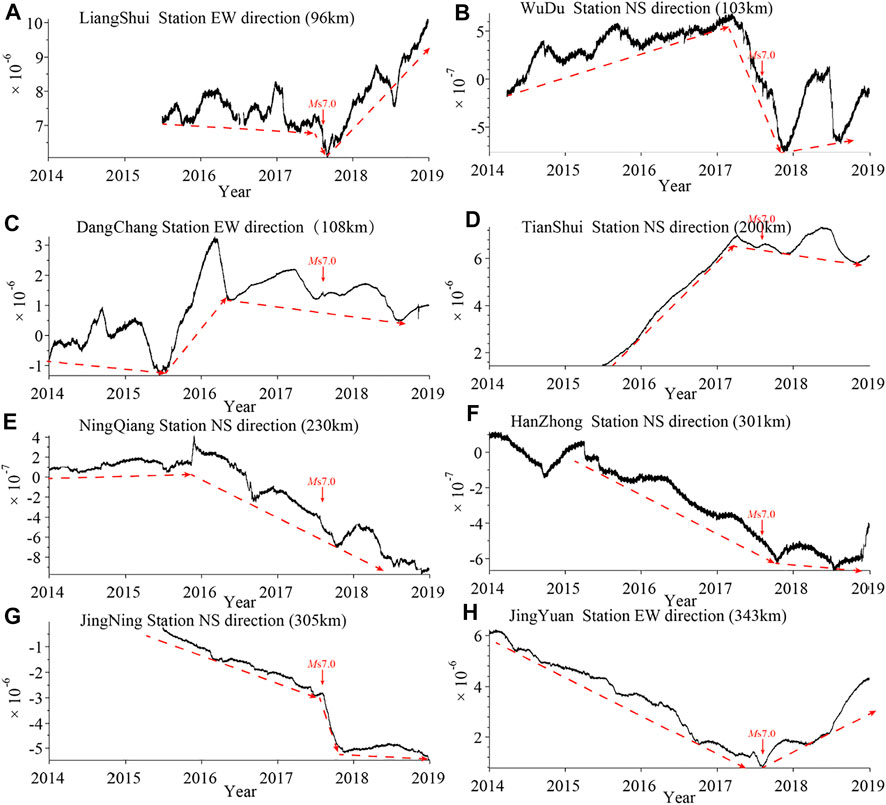
FIGURE 2. Time series curves of strain observations at eight stations near the epicenter.

2.2 Methods

Yin et al. (2000) used the Benioff strain of small earthquakes as the loading/unloading response in the LURR calculations in different tectonic settings (California, United States, and Kanto region, Japan). Yu et al. (2021) proposed a new attempt by using water levels as calculation data and achieved a good application effect. The results of the studies prove that LURR anomalies are relatively significant prior to different earthquakes, that is, the stress accumulation before an earthquake in the seismogenic region will lead to the change of the Benioff strain and water level. As a result, our approach is founded on the premise that the cracks generated by the establishment of the criticality of an earthquake may change the strain observation during the loading and unloading phases induced by earth tide. As shear stress can usually produce cracks in rock (Byerlee 1978), in this study, like other scholars (Yin et al., 2008; Yu et al., 2015; Yu et al., 2020), stress change of source media is determined by using the Coulomb failure stress (CFS) caused by earth tide in the tectonically preferred slip direction on certain slip surface (refer the calculation process in the supplement for details). The loading phase and unloading phase will be distinguished by the angle between the tidal-effective shear stress and the tectonic-effective shear stress. When the angle is less than 90°, it will be a loading phase. When the angle is greater than 90°, the two shear stress cancel each other and will be in the unloading phase. The LURR method can be simply defined as $Y=\frac{X+}{X- }$, where “+” and “−” refer to the loading phase and unloading phase, and X is the response rate (Yin et al., 1995; Yin et al., 2000). We calculate the loading (1.0)/unloading (−1.0) state of each strain observation data and the values of strain recorded during the corresponding time period. In this study, we take the hourly value of strain observation as the input data. Then, LURR is calculated by the average values of strain recorded in corresponding periods:

where H_i is strain observation at the ith record, and N+ or N− represents the numbers of records during the loading phase and unloading phase, respectively. The time window used to calculate the LURR value typically contains multiple loading–unloading cycles (Yu et al., 2021).

The strain observations may be affected by monitoring instruments and environmental impact, which will lead to some types of errors. Therefore, the following procedure is needed to preprocess the strain data in order to improve the quality of the LURR calculation. First, data with an observation period longer than 3 years are selected to ensure the stability of the instrument. Then, linear interpolation is performed for the missing data in the strain observation sequences. Finally, remove data extremes from the strain observation sequences, like the “step-change” caused by the instrument adjustment. These preprocessing procedures are quite important because short-term non tidal changes may directly affect the LURR calculation results. A total of 32 stations (13 cave strainmeter stations, 12 four-gauge borehole strainmeter stations, and seven volumetric borehole strainmeter stations) with 81 items of strain observation data are obtained, and part of the processed data is shown in Figure 2.

3 Application to Strain Data

We calculated the LURR time series results of 81 items and obtained the spatial distribution results of different stations by further interpolation, as shown in Figure 3. The calculation time window length is 1 month, the sliding step length is 1 month, and the friction coefficient is 0.4 (Yu et al., 2020; Yu et al., 2021). The selection of time window should not only consider the stability of calculation results but also identify anomalies before an earthquake. By comparing different time windows, we finally determined the time window to 1 month (Supplementary Figure S2).

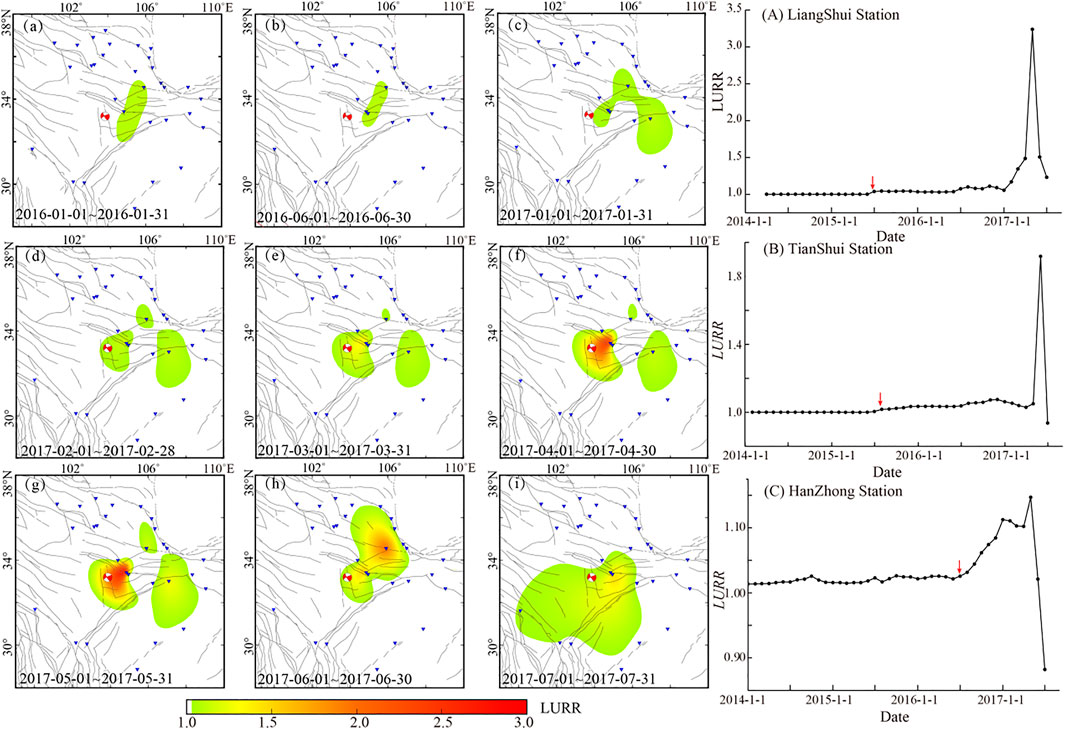
FIGURE 3. LURR spatial distribution (a–i) and LURR time series of different stations (A–C). (a–i) Spatial distribution of some periods from January 2016 to July 2017; Blue triangle: strain stations; Red focal mechanism solution: JZGEQ; Gray lines: fault. (A–C) LURR time series results for the L-Sh station, T-Sh station, and H-Zh station, respectively. Parameters for LURR evaluation are as follows: strike = 151, dip = 85, rake = 0, and depth = 15 km (Sun et al., 2018); Red arrow: start time of the anomaly.

By comparing the LURR time series obtained from strain observations at different stations (Figures 3A–C), we can find significant anomalies prior to JZGEQ. The LURR value of the three stations fluctuates around 1.0 in the initial period (January 2014–July 2016). Then, the LURR value begins to increase above 1.0 gradually from 6 months to 1 year before the occurrence of JZGEQ, reaching the maximum value in 1 to 3 months before the earthquake and subsequently returning to a low level prior to the earthquake. The trend of the LURR time series is similar to that of the previous calculation of LURR using small earthquakes and groundwater level (Yin et al., 2000; Yu et al., 2021), which indicates that the LURR method based on strain observation can better extract the pre-seismic anomalies. On the other hand, under the influence of station distribution, epicentral distance, and observation instruments, there are still noticeable differences between the LURR curves. We also find this phenomenon that the magnitude of LURR anomalies decreases with the epicentral distance, the shorter the epicentral distance, the greater the LURR value. The LURR peak value of the L-Sh station before JZGEQ is 3.2, about 96 km away from the epicenter.

The LURR spatial distribution of all the stations in Figures 3a–i shows that the northeast margin of the Tibet plateau, a region with relatively concentrated stress, has witnessed LURR anomalies since 2016, which proves that microfracture caused by stress enhancement may exist in this region. After January 2017, the range of the LURR anomalies began to expand gradually. The T-Sh station located in the northern margin of the XiQinLing fault and H-Zh station located in the QingChuan fault show the phenomenon of increasing LURR successively. This means that during this period of time, the cracks gradually extend from the epicenter of JZGEQ to the peripheral area, and this dilatancy phenomenon is consistent with the process of the “linear elasticity—dilatation” stage with the increase of load before the rock reaches the peak stress (Wawersik and Brace, 1971; Scholz and Sykes, 1973). Subsequently, the LURR anomalies magnitude of stations near the epicenter of JZGEQ begins to increase significantly, indicating that the rupture of the rocks near the epicenter began to intensify. JZGEQ occurs as the magnitude of the anomalies decreases. From the temporal and spatial evolution characteristics of the LURR anomalies, we can clearly see the process of “extension—enhance—weaken” in the epicenter and its peripheral area before the occurrence of the JZGEQ.

4 Discussion

In view of the pre-seismic stain transition and the LURR anomalies mainly concentrated in the northeast of the epicenter, and the directions with the most significant transition are mostly perpendicular to or large-angle oblique to the surrounding faults. In order to explore the relationship between pre-seismic anomalies and the seismogenesis mechanism. We further calculate the stress change induced by JZGEQ, especially the normal stress changes, based on the slip model of JZGEQ.

4.1 The Normal Stress Changes Induced by the JZGEQ

After JZGEQ, numerous academic institutions have employed far-field body wave inversion to analyze the rupture process. The GCMT solution shows that the rupture of JZGEQ is mainly dominated by strike-slip motion, and the rupture also contains ∼10% of thrusting NDCP components. With the continuous application of GNSS, InSAR, and other geodetic data, the improvement of the ground deformation constraints has gradually modified and refined the seismic rupture model (Sun et al., 2018; Liu et al., 2019; Zheng et al., 2020). Liu et al. (2019) unified the slip model into one fault, and Zheng et al. (2020) divided the rupture fault into northern and southern parts according to the distribution of aftershocks. Sun et al. (2018) analyzed multiple InSAR data pairs covering the Jiuzhaigou region and adopted an MPNT inversion to the teleseismic data set. Finally, a fault model with three segments is obtained (Figures 4A,B). The rupture propagates bilaterally on the main fault plane (Segment 1), resulting in three concentrated slip zones in Figure 4C, and Segment 2 is a thrusting segment with a slip amount of about 2 m. In this study, we use this fault model with three segments to calculate the stress changes of the surrounding faults caused by JZGEQ.

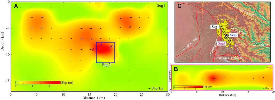
FIGURE 4. Fault plane solution geometry and slip distribution (Sun et al., 2018). (A) Slip distribution on Segment 1 and Segment 2. Red pentagram: epicenter of JZGEQ. (B) Slip distribution on Segment 3. (C) Three fault segments are plotted in black, blue, and pink boxes, respectively. The distribution of aftershock seismicities is plotted as yellow filled dots. Slip directions are plotted with arrows for every subfault, respectively.

In order to obtain the stress changes around the stations induced by JZGEQ, we collect focal mechanism solutions of historical earthquakes (cite from GCMT) and the achievements in the study area (Kirby et al., 2007; Ren et al., 2013a; Ren et al., 2013b; Cheng et al., 2018) to determine the main receiving fault rupture parameters (mainly for dip and rake angles of faults). The strike parameters of faults are calculated based on the surface outcrop results. The calculated receiving faults are shown in Figure 5B, and the rupture parameters are shown in Table 1. As aforementioned, the directions with the most significant transitions are mostly perpendicular to or large-angle oblique to the surrounding faults. This means that stress changes perpendicular to the faults has a more significant effect on strain observations. Therefore, we use the aforementioned slip model (Sun et al., 2018) to calculate the normal stress changes of faults induced by JZGEQ through PSGRN/PSCMP software (Wang et al., 2006). As we all know that most strain observations are surface observations (with depths less than 200 m), so we mainly calculate the normal stress changes of faults at the surface. The parameters of the lithospheric stratification in this study are shown in Table 2 (Cheng et al., 2018; Yue et al., 2021).

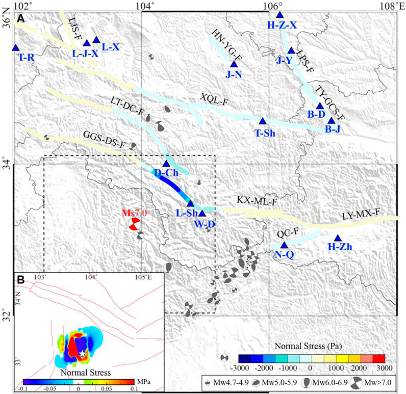
FIGURE 5. Surface co-seismic normal stress changes induced by JZGEQ. (A) Results of the source area. White pentagram: epicenter of JZGEQ; Red lines: faults. (B) Results of the receiving faults. Blue triangle: strain stations; Gray focal mechanism solution: history earthquake since 1976 (cite from GCMT), including four sizes, 4.7 ≤ MW < 4.9, 5 ≤ MW < 5.9, 6 ≤ MW < 6.9, and MW > 7; Red focal mechanism solution: JZGEQ; The colored lines: receiving faults; GGS-DS-F: GuangGaiShan–DieShan fault; LT-DC-F: LinTan-DangChang fault; KX-ML-F: KangXian-Mianlue fault; QC-F: QingChuan fault; LY-MX-F: LueYang–MianXian fault; XQL-F: North margin of XiQinLing fault; TY-GCS-F: TaoYuan-GuiChuanSi fault; LPS-F: East margin of LiuPanShan fault; HN-YG-F: HuiNing-YiGang fault; LJS-F: LaJiShan fault.

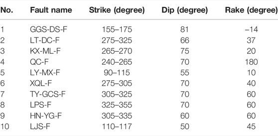
TABLE 1. Receiving fault rupture parameter in this study.

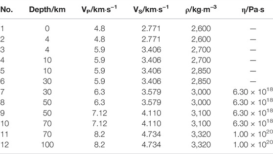
TABLE 2. Parameters of the lithospheric-layered structure model.

According to the Coulomb rupture criterion, the Coulomb stress change (△CFS) caused by seismic dislocation on a particular fault is:

where $\mathrm{\Delta }\text{τ}$ is the shear stress change (take the sliding along the strike as positive), $\mathrm{\Delta }{\text{σ}}_{\text{n}}$ denotes the normal stress change (make the fault unlock as positive), $\mathrm{\Delta }\text{P}$ represents the pore pressure change of the fault (compression is positive), and $\text{μ}$ is the friction coefficient (range from 0 to 1). In the actual calculation process, △CFS is proposed to calculate the absolute value of the shear stress on a fault (Shi and Cao, 2010). By merging the second half of Eq. 2, they introduce the “effective” friction coefficient (including the pore fluid and the medium characteristics on the fault), and the calculation formula becomes:

where ${\text{μ′}}^{}$ basically ranges from 0 to 0.75, and the value is generally selected as 0.4 in previous studies (Freed and Lin, 1998; Freed and Lin, 2001; Lei et al., 2013; Shao et al., 2016).

We calculate the co-seismic normal stress change distribution results of the source area (Figure 5A) and receiving faults Figure 5B. The receiving fault parameters in the source area are consistent with the JZGEQ rupture parameters in the study of Sun et al. (2018) (strike 151, dip 85, and rake 0). First of all, the calculation results of the source area show that the rupture of JZGEQ forms a significant negative normal stress change zone in the northeast and southwest directions of the main rupture zone. That means that the earthquake produced significant normal stress release in two directions perpendicular to the rupture fault, especially in the northeast side. The accumulation of normal stress between different faults may be adjusted with the variation of the earthquake preparation process, and this transition is likely to be captured by strain observation. This may be the reason why the strain transitions appear mainly in the northeast of the epicenter. Because of no strain observation in the southwest direction of the epicenter, we further calculate the normal stress changes of faults around the strain stations in the northeast side. The distribution of the receiving faults with negative normal stress changes is consistent with the direction of the source area, like GGS-DS-F, LT-DC-F, XQL-F, TY-GCS-F, LPS-F, HN-YG-G, and QC-F, which are mainly distributed in the northeast direction of the earthquake. As a result, the red strain stations marked in Figure 1B with significant pre-seismic and post-seismic strain transitions have excellent consistency with the calculated faults with negative normal stress changes, which indicates that the pre-seismic or post-seismic transitions observed by the strain stations are closely related to JZGEQ. That further means the LURR anomalies based on the strain observations are mainly due to the continuous cracks caused by the increase of normal stress before JZGEQ in those areas. This is consistent with the results obtained by other scholars based on the Benioff strain that the pre-seismic anomalies are distributed in the northeast of the epicenter (Yu et al., 2020).

4.2 Difference of Anomaly Characteristics

Due to the special seismogenic mechanism of this earthquake, the normal stress increases in the northeast of the epicenter before JZGEQ, namely, the faults are in the process of decoupling, and microfracture may exist in the stage of rock dilatancy. The observed results in those area is quite similar to the significant tensile pulses of ground stress normal to the fault zone in Douhe and Zhaogezhuang stations before the M7.8 Tangshan, China, earthquake in 1976 (Qiu et al., 1998). Their calculation results display that when the fracture front passes through the measuring point, the stress normal to the fracture will first rise and then drop. When the stress is at an angle of 30°, the observed change is not obvious. The strain equipment near the epicenter of JZGEQ provides lots of reliable pre-seismic and post-seismic data for the study of stress change. However, the anomaly characteristics of strain curves are different from those of LURR. The strain observation curves show pre-seismic or post-seismic transition, reflecting the effect of regional stress adjustment to a certain extent. Through the strain observation curves, we can better capture the general area of the future earthquake. But it is still difficult to predict the rupture degree of rocks in the crust. Assuming that the stations are densely distributed, we can even catch the rapid change of the strain before an earthquake at the stations close to the epicenter (such as L-Sh and W-D stations). However, considering the station density, it is difficult for us to accurately predict the rupture degree of source media by using only one or two strain observation curves, so as to accurately predict the time and location of the earthquake. In contrast, the LURR anomaly evolution process is more continuous regardless of time series curve or spatial and temporal distribution characteristics. The LURR anomalies mostly appear 6 months to 1 year before the occurrence of JZGEQ, then the amplitude of the anomalies gradually increases with time, and the earthquake occurs after the anomaly reaches the peak and falls back. The temporal and spatial distribution of the LURR anomalies also shows an evolution process of “extension—enhance—weaken” over time, which is consistent with the process of the “linear elasticity–dilatation” stage with the increase of load before the rock reaches the peak stress (Wawersik and Brace, 1971; Scholz and Sykes, 1973). The LURR method based on strain observation is an effective method to describe the dynamic change of the constitutive relationship of the source media in the crust. When we identify the rock rupture process caused by stress loading using the LURR method based on strain observation, we should pay more attention to the future seismic risk in these areas. Earthquake usually occurs after the recovery of the LURR anomaly.

5 Conclusion

The strain stations near the epicenter area of JZGEQ show us obvious pre-seismic and post-seismic transitions, which may be related to the significant enhancement of normal stress in the northeast direction of the epicenter before the earthquake. By calculating the ratio between the strain observations during the loading phase and the unloading phase induced by earth tides, anomalies might be found before JZGEQ. From the LURR curves, anomalies of LURR above 1.0 begin to appear in the surrounding stations successively from 6 months to 1 year prior to the occurrence of JZGEQ. The anomalies reach their peak value in 1–3 months before JZGEQ and eventually fall back to about 1.0 prior to the earthquake. In addition, the evolution characteristics of the LURR spatial and temporal anomalies are consistent with the process of the “linear elasticity—dilatation” stage with the increase of load before the rock reaches the peak stress, which proves that the LURR method based on strain observation is an effective way to describe the dynamic change of the constitutive relationship of the source media in the crust. The analysis of the anomalies in the corresponding LURR time series may help us estimate the location and time of an earthquake in the future.

Data Availability Statement

The original contributions presented in the study are included in the article/Supplementary Material; further inquiries can be directed to the corresponding author.

Author Contributions

CY: conceptualization, writing—original draft, and writing—review and editing. PJ, YW, and HY: manuscript revision. JC: data processing. CYu and YM: software and methodology. All authors have read and agreed to the published version of the manuscript.

Funding

This work was supported by the Joint Funds of the National Natural Science Foundation of China (U2039205) and the Spark Program of Earthquake Technology of CEA (XH20070Y and XH22040D).

Conflict of Interest

The authors declare that the research was conducted in the absence of any commercial or financial relationships that could be construed as a potential conflict of interest.

Publisher’s Note

All claims expressed in this article are solely those of the authors and do not necessarily represent those of their affiliated organizations, or those of the publisher, the editors, and the reviewers. Any product that may be evaluated in this article, or claim that may be made by its manufacturer, is not guaranteed or endorsed by the publisher.

Acknowledgments

Authors thank Dr. Liu Yue (Institute of Earthquake Forecasting, China Earthquake Administration) for her help in the calculation process, Wang et al. (2006) for sharing PSGRN/PSCMP software, and Sun et al. (2018) for sharing the slip model in the article.

Supplementary Material

The Supplementary Material for this article can be found online at: https://www.frontiersin.org/articles/10.3389/feart.2022.881884/full#supplementary-material

References

Cheng, J., Yao, S. H., Liu, J., Yao, Q., Gong, H. L., and Long, H. Y. (2018). Viscoelastic Coulomb Stress of Historical Earthquakes on the 2017 Jiuzhaigou Earthquake and the Subsequent Influence on the Seismic Hazards of Adjacent Faults. Chin. J. Geophys. 61 (5), 2133–2151. (in Chinese). doi:10.6038/cjg2018L0609
Ekström, G., Nettles, M., and Dziewoński, A. M. (2012). The Global CMT Project 2004-2010: Centroid-Moment Tensors for 13,017 Earthquakes. Phys. Earth Planet. Interiors. 200-201, 1–9. doi:10.1016/j.pepi.2012.04.002
Freed, A. M., and Lin, J. (2001). Delayed Triggering of the 1999 Hector Mine Earthquake by Viscoelastic Stress Transfer. Nature 411 (6834), 180–183. doi:10.1038/35075548
Freed, A. M., and Lin, J. (1998). Time-dependent Changes in Failure Stress Following Thrust Earthquakes. J. Geophys. Res. 103 (B10), 24393–24409. doi:10.1029/98jb01764
Kirby, E., Harkins, N., Wang, E., Shi, X., Fan, C., and Burbank, D. (2007). Slip Rate Gradients along the Eastern Kunlun Fault. Tectonics 26 (2), TC20101–TC201016. doi:10.1029/2006tc002033
Lei, X. L., Ma, S. L., and Su, J. R. (2013). Inelastic Triggering of the 2013 Mw6.6 Lushan Earthquake by the 2008 Mw7.9 Wenchuan Earthquake. Seismol. Geol. 35 (2), 411–422. (in Chinese). doi:10.3969/j.issn.0253-4967.2013.02.019
Liu, G., Xiong, W., Wang, Q., Qiao, X., Ding, K., Li, X., et al. (2019). Source Characteristics of the 2017 Ms 7.0 Jiuzhaigou, China, Earthquake and Implications for Recent Seismicity in Eastern Tibet. J. Geophys. Res. Solid Earth. 124, 4895–4915. doi:10.1029/2018JB016340
Liu, Y., and Yin, X.-c. (2018). A Dimensional Analysis Method for Improved Load-Unload Response Ratio. Pure Appl. Geophys. 175 (2), 633–645. doi:10.1007/s00024-017-1716-6
Nie, Z., Wang, D.-J., Jia, Z., Yu, P., and Li, L. (2018). Fault Model of the 2017 Jiuzhaigou Mw 6.5 Earthquake Estimated from Coseismic Deformation Observed Using Global Positioning System and Interferometric Synthetic Aperture Radar Data. Earth Planets Space. 70, 55. doi:10.1186/s40623-018-0826-4
Qiu, Z. H., Zhang, B. H., Huang, X. N., and Ge, L. (1998). On the Cause of Ground Stress Tensile Pulses Observed before the 1976 Tangshan Earthquake. Bull. Seismol. Soc. Am. 88 (4), 989–994. doi:10.1785/BSSA0880040989
Ren, J., Xu, X., Yeats, R. S., Zhang, S., Ding, R., and Gong, Z. (2013b). Holocene Paleoearthquakes of the Maoergai Fault, Eastern Tibet. Tectonophysics. 590 (1), 121–135. doi:10.1016/j.tecto.2013.01.017
Ren, J., Xu, X., Yeats, R. S., and Zhang, S. (2013a). Millennial Slip Rates of the Tazang Fault, the Eastern Termination of Kunlun Fault: Implications for Strain Partitioning in Eastern Tibet. Tectonophysics. 608 (1), 1180–1200. doi:10.1016/j.tecto.2013.06.026
Scholz, C. H., Sykes, L. R., and Aggarwal, Y. P. (1973). Earthquake Prediction: A Physical Basis. Science. 181, 803–810. doi:10.1126/science.181.4102.803
Shao, Z., Xu, J., Ma, H., and Zhang, L. (2016). Coulomb Stress Evolution over the Past 200years and Seismic Hazard along the Xianshuihe Fault Zone of Sichuan, China. Tectonophysics. 670, 48–65. doi:10.1016/j.tecto.2015.12.018
Shen, Z.-K., Sun, J., Zhang, P., Wan, Y., Wang, M., Bürgmann, R., et al. (2009). Slip Maxima at Fault Junctions and Rupturing of Barriers during the 2008 Wenchuan Earthquake. Nat. Geosci. 2 (10), 718–724. doi:10.1038/ngeo636
Shi, Y. L., and Cao, J. L. (2010). Some Aspects in Static Stress Change Calculation: Case Study on Wenchuan Earthquake. Chin. J. Geophys. 53 (1), 102–110. (in Chinese). doi:10.1002/cjg2.1473
Sun, J., Yue, H., Shen, Z., Fang, L., Zhan, Y., and Sun, X. (2018). The 2017 Jiuzhaigou Earthquake: A Complicated Event Occurred in a Young Fault System. Geophys. Res. Lett. 45, 2230–2240. doi:10.1002/2017GL076421
Wang, M., and Shen, Z. K. (2020). Present‐Day Crustal Deformation of Continental China Derived from GPS and its Tectonic Implications. J. Geophys. Res. Solid Earth. 125 (2), e2019JB018774. doi:10.1029/2019JB018774
Wang, Q., Xu, X., Jiang, Z., and Suppe, J. (2020). A Possible Precursor Prior to the Lushan Earthquake from GPS Observations in the Southern Longmenshan. Sci. Rep. 10, 20833. doi:10.1038/s41598-020-77634-6
Wang, Q., Zhang, P.-Z., Freymueller, J. T., Bilham, R., Larson, K. M., Lai, X. a., et al. (2001). Present-day Crustal Deformation in China Constrained by Global Positioning System Measurements. Science. 294 (5542), 574–577. doi:10.1126/science.1063647
Wang, R., Lorenzo-Martín, F., and Roth, F. (2006). PSGRN/PSCMP-a New Code for Calculating Co- and Post-seismic Deformation, Geoid and Gravity Changes Based on the Viscoelastic-Gravitational Dislocation Theory. Comput. Geosciences. 32 (4), 527–541. doi:10.1016/j.cageo.2005.08.006
Wawersik, W. R., and Brace, W. F. (1971). Post-failure Behavior of a Granite and Diabase. Rock Mech. 3 (2), 61–85. doi:10.1007/bf01239627
Yin, X.-C., Chen, X.-z., Song, Z.-p., and Yin, C. (1995). A New Approach to Earthquake Prediction: The Load/Unload Response Ratio (LURR) Theory. Pageoph. 145, 701–715. doi:10.1007/bf00879596
Yin, X.-C., Zhang, L.-P., Zhang, Y., Peng, K., Wang, H., Song, Z., et al. (2008). The Newest Developments of Load-Unload Response Ratio (LURR). Pure Appl. Geophys. 165, 711–722. doi:10.1007/s00024-008-0314-z
Yin, X. C. (1987). A New Approach to Earthquake Prediction. Earthq. Res. China. 3, 1–7. (in Chinese). doi:10.1007/978-3-540-47571-2_2
Yin, X. C., Wang, Y. C., Peng, K. Y., Bai, Y. L., Wang, H. T., and Yin, X. F. (2000). Development of a New Approach to Earthquake Prediction: Load/Unload Response Ratio (LURR) Theory. Pure Appl. Geophys. 157, 2365–2383. doi:10.1007/pl00001088
Yu, H.-z., Zhou, F., Cheng, J., Wan, Y.-g., and Zhang, Y.-x. (2015). The Sensitivity of the Loa/Unload Response Ratio and Critical Region Selection before Large Earthquakes. Pure Appl. Geophys. 172 (8), 2203–2214. doi:10.1007/s00024-014-0903-y
Yu, H.-Z., and Zhu, Q.-Y. (2010). A Probabilistic Approach for Earthquake Potential Evaluation Based on the Load/Unload Response Ratio Method. Concurr. Comput. Pract. Exper. 22, 1520–1533. doi:10.1002/cpe.1509
Yu, H., Yu, C., Ma, Y., Zhao, B., Yue, C., Gao, R., et al. (2021). Determining Stress State of Source Media with Identified Difference between Groundwater Level during Loading and Unloading Induced by Earth Tides. Water. 13, 2843. doi:10.3390/w13202843
Yu, H., Yu, C., Ma, Z., Zhang, X., Zhang, H., Yao, Q., et al. (2020). Temporal and Spatial Evolution of Load/unload Response Ratio before the M7.0 Jiuzhaigou Earthquake of Aug. 8, 2017 in Sichuan Province. Pure Appl. Geophys. 177, 321–331. doi:10.1007/s00024-019-02101-x
Yu, H. Z., Shen, Z. K., Wan, Y. G., Zhu, Q. Y., and Yin, X-C. (2006). Increasing Critical Sensitivity of the Load/Unload Response Ratio before Large Earthquakes with Identified Stress Accumulation Pattern. Tectonophysics. 428 (1-4), 87–94. doi:10.1016/j.tecto.2006.09.006
Yue, C., Qu, C. Y., and Niu, A. F. (2021). Analysis of Stress Influence of Qinghai Maduo Ms7.4 Earthquake on Surrounding Faults. Seismol. Geol. 43 (5), 1041–1059. (in Chinese). doi:10.3969/j.issn.0253-4967.2021.05.001
Zhang, Y., Xiang-Chu, Y., and Peng, K. (2004). Spatial and Temporal Variation of LURR and its Implication for the Tendency of Earthquake Occurrence in Southern California. Pure Appl. Geophys. 161, 2359–2367. doi:10.1007/978-3-0348-7875-3_17
Keywords: strain observation, LURR, Jiuzhaigou earthquake, normal stress, earth tide
Citation: Yue C, Ji P, Wang Y, Yu H, Cui J, Yu C and Ma Y (2022) Evolution Characteristics and Mechanism of the Load/Unload Response Ratio Based on Strain Observation Before the Jiuzhaigou MS7.0 Earthquake. Front. Earth Sci. 10:881884. doi: 10.3389/feart.2022.881884
Received: 23 February 2022; Accepted: 10 May 2022;
Published: 21 June 2022.
Edited by:
Giovanni Martinelli, National Institute of Geophysics and Volcanology, ItalyReviewed by:
Alexey Lyubushin, Institute of Physics of the Earth (RAS), RussiaCataldo Godano, University of Campania Luigi Vanvitelli, Italy
Copyright © 2022 Yue, Ji, Wang, Yu, Cui, Yu and Ma. This is an open-access article distributed under the terms of the Creative Commons Attribution License (CC BY). The use, distribution or reproduction in other forums is permitted, provided the original author(s) and the copyright owner(s) are credited and that the original publication in this journal is cited, in accordance with accepted academic practice. No use, distribution or reproduction is permitted which does not comply with these terms.
*Correspondence: Chong Yue, yuechong@seis.ac.cn