Uncertainty Analysis of Axial Pile Capacity in Layered Soils by the Piezocone Penetration Test

Lin, Jun; Hou, Xinyu; Cai, Guojun; Liu, Songyu

doi:10.3389/feart.2022.861086

ORIGINAL RESEARCH article

Front. Earth Sci., 11 April 2022
Sec. Geohazards and Georisks
Volume 10 - 2022 | https://doi.org/10.3389/feart.2022.861086

Uncertainty Analysis of Axial Pile Capacity in Layered Soils by the Piezocone Penetration Test

Jun Lin^1,2

Xinyu Hou^1,2* www.frontiersin.org

Guojun Cai^2,3 www.frontiersin.org

Songyu Liu²

¹School of Architecture and Civil Engineering, Jiangsu Open University, Nanjing, China
²Institute of Geotechnical Engineering, Southeast University, Nanjing, China
³School of Civil Engineering, Anhui Jianzhu University, Hefei, China

This study presented a framework for uncertainty analysis of the ultimate axial bearing capacity of piles evaluated by the UniCone method in layered soils. The UniCone method by Eslami and Fellenius (1997) is a direct piezocone penetration test (CPTU) method for evaluating the ultimate axial capacity of piles in the reliability design. The spatial variability of CPTU data is modeled as a random field for each soil unit in the soil strata. The empirical correlation coefficients of the UniCone method are assumed to follow lognormal distributions. On the basis of uncertainties of CPTU data and empirical correlation coefficients, the first-order reliability method (FORM) is then applied to the reliability analysis of ultimate axial bearing capacity of piles. The effects of spatial variability of CPTU data and variations of empirical correlation coefficients on the ultimate axial bearing capacity of piles are evaluated by an Excel spreadsheet-based framework. Seven case studies show that the proper identification of different soil units from soil profiles is crucial for estimating the failure probability of pile capacity in the reliability analysis. Uncertainties of CPTU data and empirical correlation coefficients would be over-estimated unless different soil units in soil profiles are identified properly from each other. The over-estimated geotechnical parameters contribute to a higher failure probability of pile capacity. The proposed framework can evaluate the uncertainty of the ultimate axial bearing capacity of pile foundations more rationally.

Introduction

Pile foundations are widely used to support highway bridges, tall buildings, transmission towers, and other structures to transfer the upper loads into stiff soil or rock layers in the deep ground (Naggar, 2002; Basack and Sen, 2014; Zhu et al., 2017; Wang et al., 2021; Basack et al., 2022). The reliability of ultimate axial bearing capacity of piles is a major safety issue for geotechnical engineering. The spatial variability of in situ measurements and variations of empirical correlations coefficients lead to significant uncertainties in predicting the ultimate axial bearing capacity of piles by the cone penetration test (CPT) or piezocone penetration test (CPTU) (Haldar and Babu, 2008; Dithinde et al., 2011; Chen and Zhang, 2013; Mendoza et al., 2017; Jarushi et al., 2020).

The reliability-based design (RBD) has been increasingly concerned as a more rational approach to evaluate the effects of geotechnical uncertainties on the ultimate axial bearing capacity of piles (Phoon and KulhawyGrigoriu, 2000; Tandjiria et al., 2000; Honjo et al., 2002; Zhang and Chu, 2009; Zhang and Chu, 2009). The first-order reliability method (FORM) has been demonstrated as one of the most effective tools for probabilistic design in geotechnical practice (Low and Tang, 1997; Haldar and Sivakumar Babu, 2009; Teixeira et al., 2012; Teixeira et al., 2014). In most FORM studies, when conducting spatial variability analysis, different soil units are seldom identified from each other in a soil profile, which may lead to a biased estimation of uncertainties associated with geotechnical and design parameters (Phoon and Kulhawy, 1999; Uzielli et al., 2005; Low and Phoon, 2015). If the layered soil strata are viewed as an integral unit, the correlation among the geotechnical parameters of different soil units in a soil profile becomes indistinct. The spatial correlation significantly influences the failure probability of geotechnical design obtained from the FORM analysis (Jaksa et al., 1997; Dithinde et al., 2011; Ching and Phoon, 2019; Wang et al., 2019). As a consequence, the probabilistic analysis of the ultimate axial bearing capacity of piles may be biased.

This study presented an Excel spreadsheet-based framework for the uncertainty analysis of the ultimate axial bearing capacity of piles in layered soils. The CPTU-based UniCone method by Eslami and Fellenius (1997) is selected to calculate the ultimate axial bearing capacity of piles by CPTU data. The framework takes into account the spatial variability of layered soils and the variations of empirical correlation coefficients of the UniCone method. The uncertainties associated with CPTU parameters and empirical correlation coefficients in layered soils are analyzed in terms of the random field and random variables, respectively. The FORM is applied to evaluate the ultimate axial bearing capacity of pile foundations considering the uncertainties of design parameters. The uncertainties of ultimate axial bearing capacity of piles in layered soils from seven case studies are discussed with the proposed framework.

Uncertainties in the UniCone Method

Many direct CPT/CPTU-based methods have been proposed to predict the ultimate axial bearing capacity of piles in geotechnical practice (Lunne et al., 1997; Mayne, 2007). Among those methods, the UniCone method by Eslami and Fellenius (1997) has been proved to be a more reasonable method than other methods (Abu–Farsakh and Titi, 2004; Cai et al., 2009; Cai et al., 2012; Niazi and Mayne, 2016; Golafzani et al., 2020; Heidari and Ghazavi, 2021). The UniCone method has shown usefulness and reliability for clays, silts, and sands (Mayne, 2007; Amirmojahedi and Abu–Farsakh, 2019). Hence, the UniCone method (Eslami and Fellenius, 1997) is adopted for the uncertainty analysis of the ultimate axial bearing capacity of piles in this research.

The ultimate axial bearing capacity (Q_u) of a single pile mainly consists of end bearing capacity (Q_b) and friction resistance along the shaft (Q_s):

Q_{u} = Q_{b} + Q_{s} = q_{b} A_{b} + Σ_{i = 1}^{N} f_{p i} A_{s i} (1)

where q_b is the unit end resistance at the pile base, A_b is the section area of the pile, f_pi is the unit pile shaft resistance of the ith soil layer, A_si is the superficial area of pile shaft at the ith soil layer, and N is the number of soil units in the soil strata.

Based on a database of 102 full-scale pile loading tests from 40 sites, Eslami and Fellenius (1997) developed the correlations between unit pile resistances and effective piezocone penetration resistance (q_e) for a single soil layer as

q_{b} = C_{p} q_{e g} (2a)

f_{p} = C_{s} q_{e} (2b)

where C_p is the toe correlation coefficient, C_s is the shaft correlation coefficient, determined from a soil behavior chart depending on sleeve frictional resistance (f_s) and q_e, q_eg is the geometric average of q_e values over the influence zone, q_e is the effective cone tip resistance that q_e = q_t–u₂, and q_t is the cone tip resistance corrected for the unequal area effect caused by pore water pressure (u₂) (Lunne et al., 1997; Mayne, 2007). Table 1 presents the empirical ranges and advised approximation for C_s corresponding to the soil type.

TABLE 1

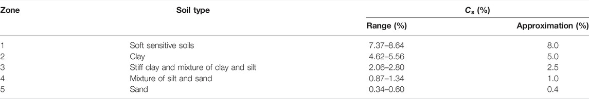
TABLE 1. Shaft correlation coefficient C_s (Eslami and Fellenius, 1997).

Substitution of Eqs 2a, 2b in Eq. 1 derives

Q_{u} = A_{b} C_{p} q_{e g} + Σ_{i = 1}^{N} A_{s i} C_{s i} q_{e i} (3)

The influence zone for q_eg values depends on the stiffness of surrounding soils above and below the pile toe along with the diameter (B) of the designed piles. Based on comprehensive literature reviews and experimental analysis, Eslami and Fellenius (1997) suggested that the influence zone extends from 4B below the pile toe to a height of 8B above the pile toe when a pile is installed through a weak soil into a dense soil, and 2B above the pile toe when a pile is installed through a dense soil into a weak soil. Due to the uncertainties associated with (C_p, q_eg, C_si and q_ei), Q_u could vary in a large range. In this research, the Unicone method is analyzed from a probabilistic way to evaluate the reliability of the ultimate axial bearing capacity of piles.

Uncertainties of Empirical Correlation Coefficients

For a soil profile with high variability, the geotechnical parameters usually followed skewed probability density distributions (PDFs). Consequently, in the estimation of bearing capacity around the pile toe, the geometric mean value is more rational than the arithmetic mean value for average properties of geotechnical parameters (Eslami and Fellenius, 1997; Golafzani et al., 2020; Heidarie Golafzani et al., 2020). However, the geometric mean, q_eg, is not compatible with reliability-based analysis, in which the arithmetic mean is used. Hence it is necessary to rewrite Eq. 3 in the form of the arithmetic mean (q_ea), as follows:

Q_{u} = A_{b} a C_{p} q_{e a} + Σ_{i = 1}^{N} A_{s i} C_{s i} q_{e i} (4)

where a = q_eg/q_ea is the ratio of geometric mean (q_eg) to arithmetic mean (q_ea), varying between 0 and 1. The values of the ratio a can be determined from the sampling CPTU data. Since both geometric and arithmetic mean values of q_e are viewed as deterministic quantities, the ratio (a) is also treated as a constant (deterministic value).

According to Eq. 4, four indices including two in situ measurements (q_ea and q_e) and two empirical coefficients (C_p and C_s) should be concerned as random parameters. The variance of Q_u depends on the probability distributions of four indices (C_p, q_ea, C_si, and q_ei), and also depends on the correlation between each pair of two indices. For convenience, the geotechnical parameters in Eq. 4 are denoted as Y variables, i.e., Y₁ = C_p, Y₂ = q_ea, Y_3i = C_si, Y_4i = q_ei, where i is the order of the soil unit. In this research, all the Y parameters in Eq. 4 are assumed to be individually following lognormal distribution advised for most geotechnical parameters. Under this assumption, only the means and variance of these parameters are needed and discussed in this section. To get a consistent description of the magnitude of uncertainty, the dimensionless coefficient of variation (COV) is used instead of variance, defined as the ratio of standard deviation over the mean.

The C_p and C_s are uncertain because the true values are not available, and only empirical values can be obtained based on the engineering database. Based on 14 pile case histories, Eslami and Fellenius (1997) proposed a mean of 0.98 and a standard deviation of 0.09 for C_p. Hence, in this research, the C_p is assumed to be a lognormal variable with a mean of 1 and COV of 0.1. For the C_s, the recommended values are shown in Table 1, most values should vary within the 95% confidence interval (CI). If the soil strata containing different layers are treated as a whole soil unit, the 95% CI for the PDF of C_s should be the interval between the lower bound and upper bound for all the involved soil types.

Figure 1 illustrated the estimated PDFs of C_s for different soil types. The statistical parameters including expected value (μ), standard deviation (σ), COV, and the 95% CI are listed in Table 2. The 95% CI for each type of soil is the same as the recommended ranges in Table 1, and the estimated mean value of C_s for each soil type approximates the suggested mean value. In Figure 1, the PDFs of C_s are almost asymmetric if different types of soils are investigated individually. The normal distribution can be used to approximate the lognormal distribution when the COV is small (COV <0.3). However, the lognormal distribution is still adopted to guarantee the positivity of C_s.

FIGURE 1

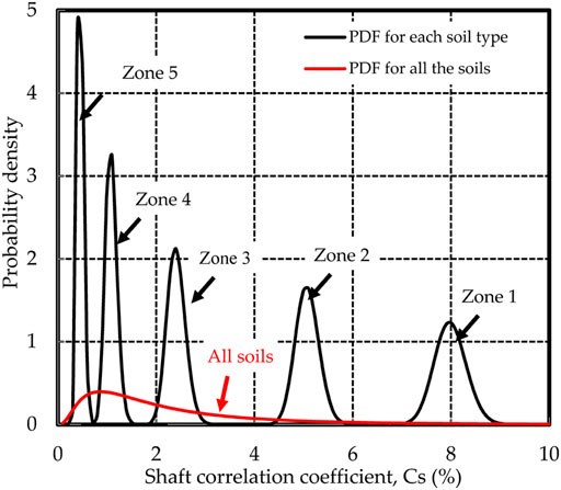
FIGURE 1. Estimated PDFs of C_s.

TABLE 2

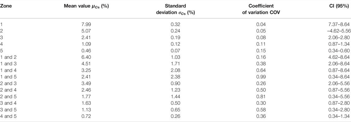
TABLE 2. Proposed lognormal distributions for C_s.

However, if different soil units are lumped together, the estimated PDFs of C_s are distinctly skewed (as shown in Figure 1) and the COVs increase significantly. In extreme cases, both Zone 1 and Zone 5 exist in the soil strata, the mean and COV of C_s are 2.41 and 0.99. Due to uncertainties associated with empirical coefficients, separating different soil units properly should be more reasonable than a mixing soil profile in the reliability-based analysis by the UniCone method. This suggestion is also suitable for other CPT/CPTU-based predicting methods (Mayne, 2007; Golafzani et al., 2020; Heidarie Golafzani et al., 2020).

Uncertainties of Effective Cone Tip Resistance

Soil properties exhibit spatial variability over the space. Due to insufficient site characterization information and limitations of testing techniques, the geotechnical parameters become variational. Different Interpretations of in situ testing data also contribute to the geotechnical uncertainty (Mo et al., 2021; Chen and Mo, 2022). The random field has been widely applied to model the spatial variability of geotechnical parameters including the effective cone tip resistance (both q_e and q_ea).

The Framework of Random Field

In a random field model, the in situ measurement Y(z) at a depth z in a soil unit is treated as a combination of a trend component t(z), and a fluctuation component w(z) (Phoon, et al., 2003; Uzielli, et al., 2005):

Y (z) = t (z) + w (z) (5)

The trend component represents the impact of physical factors on the in situ measurements, such as overburden pressure and geologic setting, usually treated as a deterministic component. The fluctuation component represents the spatial variability of a geotechnical parameter. It has been emphasized that the fluctuation component is not inherent but depends on the selection of trends (Cafaro and Cherubini, 2002; Phoon, et al., 2003; Stuedlein et al., 2012). In the reliability analysis, only the arithmetic mean value is used rather than the trend, leading to a potential conflict between reliability and the random field model. Assuming that C_s is independent of both depth (z) and q_e, it can be proved easily that a linear trend in Eqs 2a, 2b is mathematically equivalent to the arithmetic mean of q_e profile. Therefore, it is acceptable to directly apply the random field with a linear trend for the reliability-based analysis of piles. However, a high-order trend cannot be replaced by the arithmetic mean for q_e in Eqs 2a, 2b. In this case, it is advised to further subdivide the soil into different units and perform further analysis.

In a random field model, the linear trend can be determined by linear regression analysis. The scale of fluctuation (δ) represents the inherent spatial variability of a soil property. COV and δ are used to describe the corresponding fluctuation component (Phoon and Kulhawy, 1999; Phoon et al., 2003).

The Scale of Fluctuation and Spatial Averaging

The scale of fluctuation in the vertical direction (δ_v) or in the horizontal direction (δ_h) indicates that the soil property values show a relatively strong correlation within the lagging distance. This study emphasizes the vertical random field parameters as the piles are mostly installed vertically in layered soils.

The random field theory is simplified by the weak stationarity, which requires that the means and variances of the data segments in a soil profile are constant along with the coordinate (Jaksa et al., 1997). For a weak-stationary soil profile, the autocorrelation function (ACF) only depends on the intervals between two observations rather than the absolute depth coordinates (z₁ and z₂). The ACF, which is normalized by the sample variance, can be estimated as (Phoon et al., 2003; Uzielli, et al., 2005)

R (τ = j Δ z) \approx \frac{1}{s^{2} (n - j - 1)} Σ_{i = 1}^{n - j} [w (z_{i}) w (z_{i + j})] (6)

where τ is lagging distance, τ = |z₁ – z₂|; Δz is sampling interval; z_i = i(Δz) is depth coordinate of ith sampling point; n is the number of data points; and s² is the sample variance. Eq. 6 is accurate up to a maximum lag of less than 1/4 of the total sample length, i.e., j < n/4. In practice, only the initial parts of the ACF (i.e., R(τ) > 1.96/ $\sqrt{n}$ ) are necessary for subsequent analysis according to Uzielli et al. (2005). Eq. 6 should be calculated within the sampling interval smaller than the δ_v.

Discontinuity of ACF can be observed when the lag distance approaches zero, which is referred to as the nugget effect (Jaksa et al., 1997). The nugget effect describes the impacts of the random measurement error and spatial variability of soil property in a small scale and also contributes to the imprecise evaluation of uncertainties associated with geotechnical data.

The ACF obtained from Eq. 6 is discrete. Several theoretical continuous autocorrelation models (ACMs) can be used to fit the sample ACF based on the regression analysis (Phoon et al., 2003; Uzielli, et al., 2005). The best-fitting ACM should be selected to determine the δ_v of geotechnical data. Vanmarcke (1977) suggested that the variance of geotechnical data can be reduced by averaging data points within the range of δ_v. The reduced variance is more representative than the raw measurements as the performance of a single pile depends on the averaged regionalized soil property, rather than the point estimates of variance. Table 3 lists five common ACM and the corresponding variance reduction functions (VRFs), which are defined as the ratio of the variance of post-averaged data over that of pre-averaged data.

TABLE 3

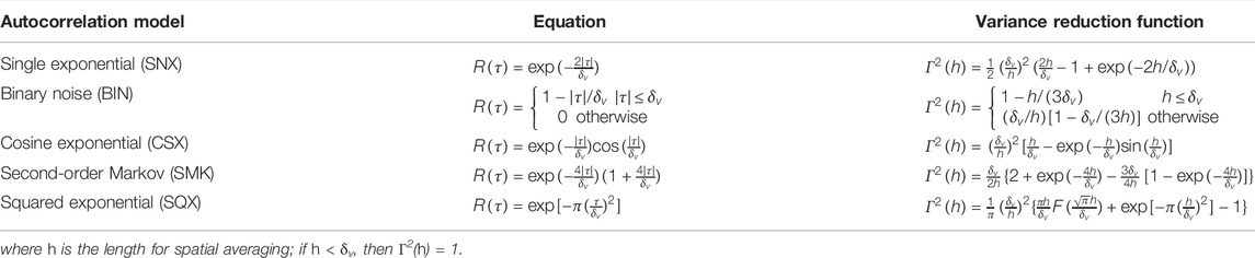
TABLE 3. Autocorrelation models and variance reduction functions (Vanmarcke, 1977; Phoon and Kulhawy, 1999); Phoon et al., 2003; Uzielli, et al., 2005).

Coefficient of Variation

The coefficient of variation evaluates the absolute magnitude of fluctuation about the trend. The COV of a soil profile in one soil unit after removing a trend is defined as (Phoon and Kulhawy, 1999)

C O V = \frac{σ_{Y}}{μ_{Y}} = \frac{\sqrt{\frac{1}{n - 1} \sum_{i = 1}^{n} {[w (z_{i})]}^{2}}}{μ_{Y}} (7)

where σ_Y and μ_Y are the standard deviation and mean of Y, n is the number of data points in the profile, and z_i is the depth of ith sampling point.

After spatial averaging, the reduced COV_r of Y in each soil unit is

C O V_{r} = \frac{\sqrt{Γ^{2} (h) σ_{Y}^{2}}}{μ_{Y}} = Γ (h) C O V (8)

Random Field Model in Layered Soils

Piles are generally installed in layered soil strata rather than homogeneous soil. For layered soil strata, the random field model can be applied for a soil profile without separating different soil units, as commonly used in geotechnical literature. However, it is suggested to apply the random field model for each soil unit since the COV of geotechnical data can be highly overestimated if different soil units are mixed up together (Phoon et al., 2003; Uzielli, et al., 2005). The autocorrelation structure can be also highly overestimated if different soil units are not identified properly. It has been observed that the estimated δ_v depends on the scale of observation (Cafaro and Cherubini, 2002). If the whole soil strata are modeled as one random field, then the q_e readings in a soil unit are merely a fluctuation component of the whole soil profile. This observation contributes to the conclusion that q_e is highly correlated in space. Even if a linear trend is removed, the CPTU readings are still close to each other at adjacent locations. If different soil units are investigated individually, the δ_v should be smaller and more representative of spatial variability of q_e.

Based on the aforementioned analysis, the random field model of soil strata containing N soil units is recommended as shown in Figure 2. The random field model is constructed individually for each soil unit, including the influence zone. The size of the influence zone directly impacts the correlations among q_ei of different soil units.

FIGURE 2

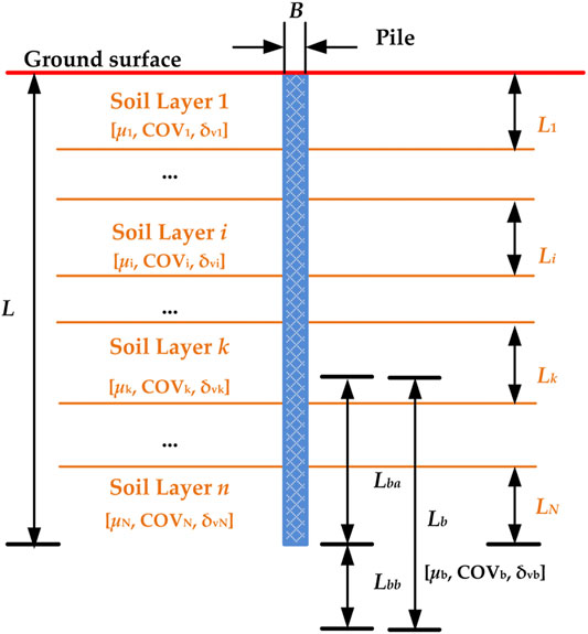
FIGURE 2. Random field model for layered soils.

Correlations Among Geotechnical Parameters

Another source of the uncertainties associated with q_e is the covariance, which describes the linear relationship between paired geotechnical parameters. For a soil profile shown in Figure 3, Vanmarcke (1977) proposed the following formula to estimate the product-moment correlation (ρ_Y12) between two segments (w_s1 and w_s2):

ρ_{Y 12} = \frac{z_{0}^{2} Γ^{2} (z_{0}) - z_{1}^{2} Γ^{2} (z_{1}) + z_{2}^{2} Γ^{2} (z_{2}) - z_{3}^{2} Γ^{2} (z_{3})}{2 Δ z_{1} Δ z_{2} \sqrt{Γ^{2} (Δ z_{1}) Γ^{2} (Δ z_{2})}} (9)

where z₀ = |c - b|; z₁ = |c - a|; z₂ = |d - a|; z₃ = |d - b|; Δz₁ = |b - a|; Δz₂ = |d - c|; a and c are the upper bounds of w_s1 and w_s2, respectively; b and d are the lower bounds of w_s1 and w_s2, respectively; and Γ²(•) is the variance reduction function of the whole profile.

FIGURE 3

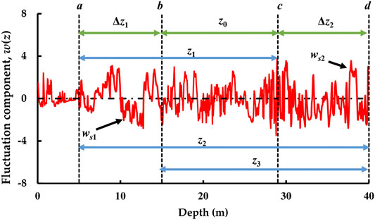
FIGURE 3. Calculation scheme of the correlation between two segments.

Vanmarcke (1977) has proven that the above equation is still applicable even if the two segments are overlapped (i.e., c > b). According to the above formula, the correlation between any two q_e profiles of non-overlapped soil units approximates to zero. But for two soil units overlapped, the correlations should not be ignored.

By applying Eq. 9, the soil profile should be stationary in the second-moment sense because the correlation structure can be described using a consistent ACM. The stationarity of a geotechnical profile can be checked rigorously using the modified Bartlett’s test proposed by Phoon et al. (2003). The non-stationary points of the soil profile may correspond to the soil boundaries. Uzielli et al. (2005) showed that cohesionless soils are more variable than cohesive soils. The variance of fluctuation components can be hardly constant with the depth caused by non-stationarity. For a single soil unit, weak stationarity is often an acceptable assumption after a specific trend is removed (Vanmarcke, 1977; Stuedlein et al., 2012; Bong and Stuedlein, 2017).

Including the uncertainties of C_p, q_ea, C_si, and q_ei, the variability of Q_u can be estimated by the random field theory. In this research, the following strategy is adopted when the N different soil units are identified properly from a soil profile:

(1) The q_e data of different soil units along the pile shaft are uncorrelated to each other, while they are autocorrelated in the same soil unit

(2) If the influence zone contains at least two soil units, then the q_ea of the influence zone is assumed to be uncorrelated to all the q_e along the pile shaft and the correlation matrix of (C_p, q_ea, C_si, q_ei) is simply an identity matrix

(3) If the influence zone is limited in the Nth soil unit, then the correlation between q_ea and q_eN is estimated using Eq. 9, whereas q_ea and q_ei (i = 1, 2, … , N-1) are uncorrelated

Reliability Index of Pile Bearing Capacity

The most advantage of reliability analysis is to quantify the uncertainties of design parameters and to manipulate those uncertainties consistently. In this section, the basic concept of reliability analysis is introduced firstly. Then, data transformation is discussed to conduct the reliability analysis. An Excel-based reliability analysis framework is illustrated to evaluate the ultimate axial bearing capacity of piles in layered soils by spatial variability and the FORM analysis.

Reliability Analysis Theory

Reliability analysis originates from the limit state design concept. The limit state function of the vertically loaded pile can be written as

M = Q_{u} - S (10)

where Q_u is the ultimate bearing capacity, S is the load, and M is the margin of safety. If Q_u and S are normally distributed, then M is also normally distributed with a mean of μ_M and a standard deviation of μ_M. If Q_u and S are further uncorrelated, then a dimensionless reliability index, β, is defined as (Baecher and Christian, 2005)

β = \frac{μ_{M}}{σ_{M}} = \frac{μ_{Q_{u}} - μ_{S}}{\sqrt{σ_{Q_{u}}^{2} + σ_{S}^{2}}} (11)

Here, M represents the geometrical distance from a design point to the limit state in the unit of capacity. Eq. 11 indicates that β is a standardized representation of M. β evaluates the distance from a design point to the failure criteria in the standardized space. Eq. 11 assumes that the margin of safety is expressed as a linear sum of uncorrelated normal random variables. However, when the M is expressed in terms of design parameters (C_p, q_ea, C_si, q_ei and S), this assumption is contradictory to the geotechnical practice, because the capacity of piles is often expressed as a nonlinear function of non-Gaussian variables. After proper data transformation, β can be directly defined in the multivariate standard normal space. So the FORM provides a more rational estimation of the probability of failure (p_f). Data transformation for each variable and the correlations among those variables are introduced in the following sections.

Data Transformation

In this research, S is also assumed as a lognormal random variable with a mean of μ_S and standard deviation of σ_S. Then, the correlated Y variables can be individually converted to correlated standard normal variables (V_i) using the following simple transformation:

β = \frac{μ_{M}}{σ_{M}} = \frac{μ_{Q_{u}} - μ_{S}}{\sqrt{σ_{Q_{u}}^{2} + σ_{S}^{2}}} (12)

where T_i = lnY_i, μ_Ti and σ_Ti are the mean value and standard deviation of T_i, respectively. The μ_Ti and σ_Ti can be obtained using (Low and Tang, 1997) the following expression:

μ_{T_{i}} = ln (μ_{Y_{i}}) - 0.5 ln (C O V_{Y_{i}}^{2} + 1) (13a)

σ_{T_{i}} = \sqrt{ln (C O V_{Y_{i}}^{2} + 1)} (13b)

where μ_Yi and σ_Yi are the mean value and standard deviation of Y_i, respectively.

Due to the nonlinear transformation, the product-moment correlation coefficient between V_i and V_j, ρ_Vij, is different from the initial correlation coefficient ρ_Yij. However, shifting or scaling two variables will not change the product-moment correlation between them. Therefore ρ_Vij should be the same as the product-moment correlation (ρ_Tij) between T_i and T_j.

Since T_i and T_j follow the normal distribution, (T_i + T_j) is still a Gaussian variable with means and variances as

μ_{T_{i} + T_{j}} = μ_{T_{i}} + μ_{T_{j}} (14a)

σ_{T_{i} + T_{j}}^{2} = σ_{T_{i}}^{2} + σ_{T_{j}}^{2} + 2 ρ_{T i j} σ_{T_{i}} σ_{T_{j}} (14b)

Therefore, Y_iY_j = exp(T_i + T_j) follows lognormal distribution with the expected value as

\begin{matrix} μ_{Y_{i} Y_{j}} = exp [μ_{T_{i}} + μ_{T_{j}} + (σ_{T_{i}}^{2} + σ_{T_{j}}^{2} + 2 ρ_{T i j} σ_{T_{i}} σ_{T_{j}}) / 2] \\ = exp [(μ_{T_{i}} + σ_{T_{i}}^{2} / 2) + (μ_{T_{j}} + σ_{T_{j}}^{2} / 2) + ρ_{T i j} σ_{T_{i}} σ_{T_{j}}] \\ = μ_{Y_{i}} μ_{Y_{j}} exp (ρ_{T i j} σ_{T_{i}} σ_{T_{j}}) \end{matrix} (14c)

Combining Eqs 13a, 13b, Eqs 14a, 14b, 14c, the following expression can be derived:

\begin{matrix} ρ_{V i j} = ρ_{T i j} = \frac{1}{σ_{T_{i}} σ_{T_{j}}} In (\frac{μ_{Y_{i} Y_{i}} - μ_{Y_{i}} μ_{Y_{j}}}{μ_{Y_{i}} μ_{Y_{j}}} + 1) = \frac{1}{σ_{T_{i}} σ_{T_{j}}} I n [\frac{cov (Y_{i}, Y_{j})}{μ_{Y_{i}} μ_{Y_{j}}} + 1] \\ = \frac{ln (ρ_{Y i j} C O V_{Y_{i}} C O V_{Y_{j}} + 1)}{\sqrt{ln (C O V_{Y_{i}}^{2} + 1) ln (C O V_{Y_{j}}^{2} + 1)}} \end{matrix} (15)

It is noted that ρ_Vij is the (i,j)th entry of correlation matrix K_V. So K_V can be determined from the correlation matrix K_Y, especially in the situation that the COVs of Y_i and Y_j are small (e.g., COV <0.3). ρ_Vij may approximate ρ_Yij because ln(1 + x) approximates x very well when x is close to zero. After obtaining the transformed correlation matrix, the last issue in Eq. 11 is that the correlated Gaussian variables need to be converted to uncorrelated Gaussian variables. Transformation for uncorrelated Gaussian variables with the definition of reliability index is introduced subsequently.

Reliability Index

The Cholesky decomposition method converts the correlated standard normal variables to uncorrelated variables with no change in the normality of the correlation matrix. Since K_V is asymmetric and positive definite matrix, it can be factored into two matrices transposing each other (Baecher and Christian, 2005):

K_{V} = W W^{T} (16a)

where W is a lower triangular matrix. Then, the vector of uncorrelated standard normal variables, X, can be obtained as

X = W^{- 1} V (16b)

where X = (X₁, X₂, … , X₅) is the vector of uncorrelated standard normal variables, V = (V₁, V₂, … , V₅).

Finally, all correlated lognormal Y variables are converted to uncorrelated standard normal X variables. Assuming that the limit state function can be approximated by the sum of transformed uncorrelated Gaussian variables, the reliability index, β, can be estimated using the following formula (Baecher and Christian, 2005):

β = \sqrt{X^{T} X} = \sqrt{V^{T} K_{V}^{- 1} V} (17)

To consistently demonstrate the sensitivity of β on Y_i, a sensitivity factor (α_i) is defined as X_i/β. A large absolute value of α_i indicates high influence of Y_i on β (Teixeira et al., 2012, Teixeira et al., 2014). The reliability index (β) defined in Eq. 17 indicates the minimal distance between the critical data point in the limit state function and the origin of uncorrelated multivariate standard normal space. Therefore, the FORM analysis becomes the problem of finding minimal β and corresponding critical design points under the constraint of limit state function.

Algorithm for Reliability Index

Many algorithms for conditional minimization are available in the statistic literature. The algorithm procedure proposed by Low and Tang (1997) can be modified to conveniently solve the minimization problem. The procedure is updated to account for the transformation of correlations among variables as follows:

1) Define the means, standard deviations, and correlation matrix (K_Y) of (Y₁, Y₂, … , Y₅) using the random field model

2) Convert Y_i to X_i individually using the logarithm transformation with a standardizing procedure, using Eq. 12, Eq. 13a, Eq. 13b

3) Convert the correlation matrix K_Y to K_V using Eq. 15

4) Assign initial values for each V_i variable and obtain the corresponding Y_i variable

5) Obtain the margin of safety, M = f(Y₁, Y₂, … , Y₅)

6) Define reliability index, β, according to Eq. 17

7) Invoke the “Solver” command in the Excel software to minimize β by changing the values of V_i subject to the constraint that M = 0

8) Obtain the critical values of (V₁, V₂, … , V₅) and corresponding β

9) Perform Cholesky decomposition on the K_V, obtain the critical values of (X₁, X₂, … , X₅) using Eqs 16a, 16b, and evaluate the sensitivity factors (α_i)

10) Estimate the probability of failure using p_f = Φ(-β)

The modified algorithm is suitable for both correlated and uncorrelated random variables. An Excel-based framework for the reliability design of pile foundations by the CPTU-based UniCone method is developed, as shown in Figure 4. Using the proposed framework, seven case studies in two sites are analyzed to investigate the difference of estimated p_f by separating soil units properly or not.

FIGURE 4

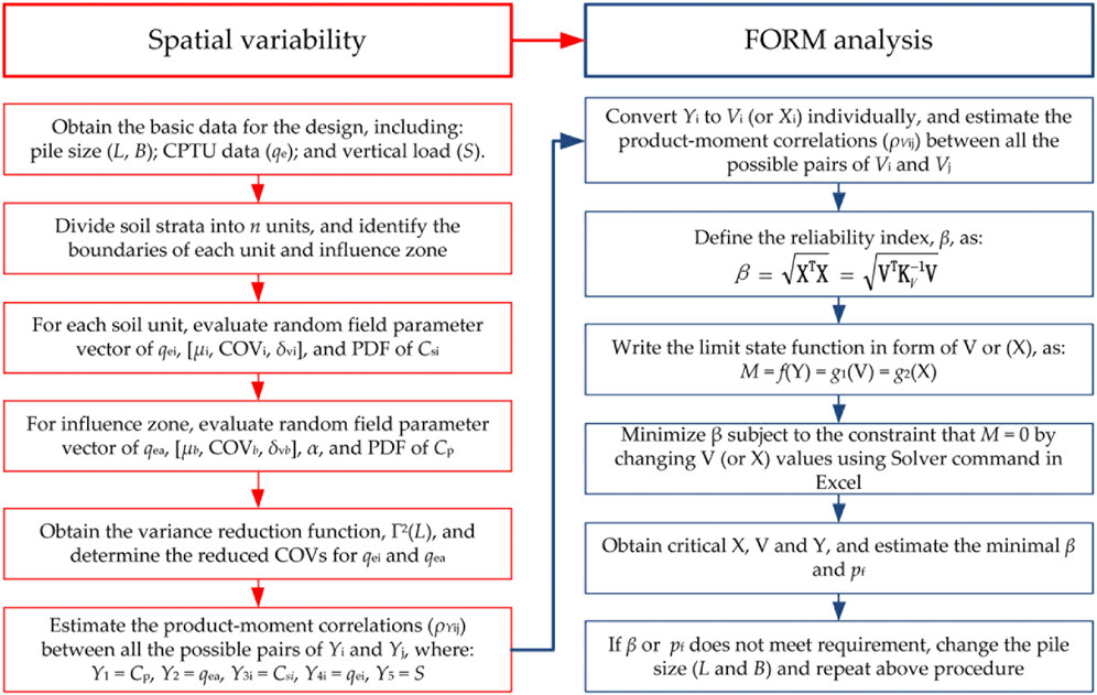
FIGURE 4. Flowchart for the uncertainty analysis of axial pile capacity in layered soils by the UniCone method.

Uncertainty Analysis of Axial Pile Capacity

The impacts of uncertainties of geotechnical parameters on the reliability design are assessed in terms of the probability of failure factor of safety (p_f–FS) curve by different interpretations of soil profiles. The FS represents the averaged influence of resistance on the load, since a large mean value of capacity with a small mean value of the load leads to a high FS. Then, the mean value of S is determined using μ_S = μ_Qu/FS. The COV of S is selected as 15% as commonly used in literature (Zhang et al., 2004; Chen and Zhang, 2013; Tang and Phoon, 2018; Bueno Aguado et al., 2021). If soil profiles are interpreted in different ways, the values of δ_v and COV should change accordingly. Deviations in β and p_f could be expected due to different values of δ_v and COV at the same FS level. Seven driven piles designed in layered soils are analyzed by the proposed framework to demonstrate the importance of identifying different soil units properly. For convenience, Type I indicates the uncertainty analysis by dealing with the soil strata as an integrated unit, while Type II indicates the uncertainty analysis by identifying different soil units from a soil profile.

Site Condition

The seven design case studies are located in Nanjing and Suqian, Jiangsu, China. Table 4 lists the dimensions and required axial capacities of the driven piles. These piles include closed-end pre-stressed high-strength concrete (PHC) pipe piles and pre-stressed concrete (PC) pile. The piles are driven into the bearing layers. The bearing layers locate in the last soil units as listed in Type II method. The pile types do not influence the estimations of bearing capacity by the UniCone method as discussed previously.

TABLE 4

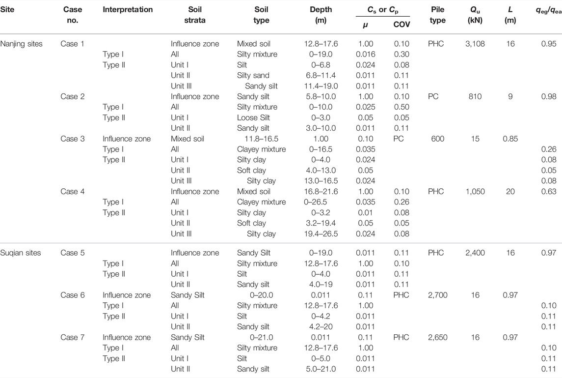
TABLE 4. Basic information of site strata and piles.

In Table 4, Case 1–Case 4 are in the Nanjing sites. In Case 1 and 2, soil strata consist of sand and silt units, while in Case 3 and 4, the soil strata consist of silty clay with soft clay. In Table 4, Case 5–Case 7 are in the Suqian sites. The soil strata in Case 5–Case 7 contain relatively loose silt over median sandy silt. Therefore, the study on Case 1 and 2 illustrates the performance of reliability-based analysis in mixed cohesionless deposits. The study on Case 3 and 4 checks the performance of reliability analysis in mixed cohesive deposits. The investigation on Case 5–7 evaluates the performance of reliability-based analysis in mixed silts. Case 1 is a representative example of q_e profile for the spatial variability analysis.

Spatial Variability Analysis

In the proposed framework, the spatial variability of q_e has been analyzed. The results of spatial analysis are concluded in Table 5. Figure 5 presents a representative example of q_e profile measured at one of the Nanjing sites in Case 1. Three soil units are identified from the CPTU profile according to the adjacent borehole data, as shown in Figure 5. The first unit is silt from the ground surface to a depth of 6.8 m. The second unit is silty sand from 6.8 to 11.4 m in depth. The last soil unit is sandy silt from 11.4 to 19.0 m in depth.

TABLE 5

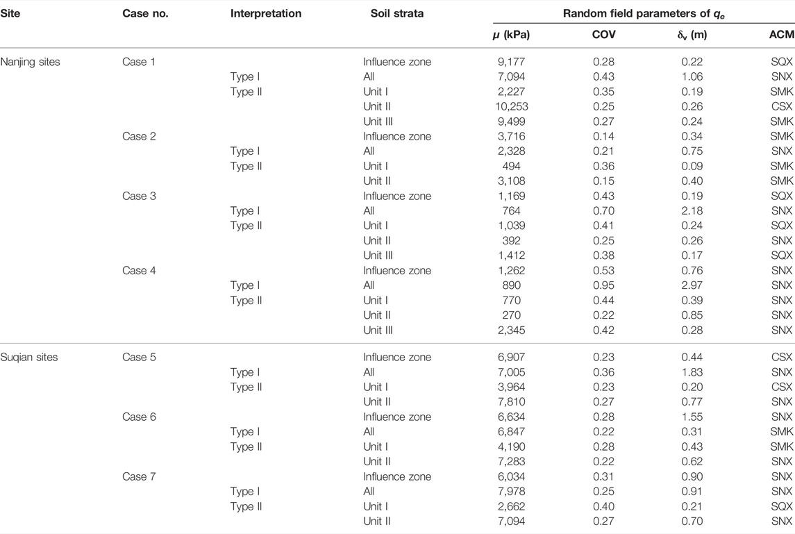
TABLE 5. The results of spatial analysis of q_e.

FIGURE 5

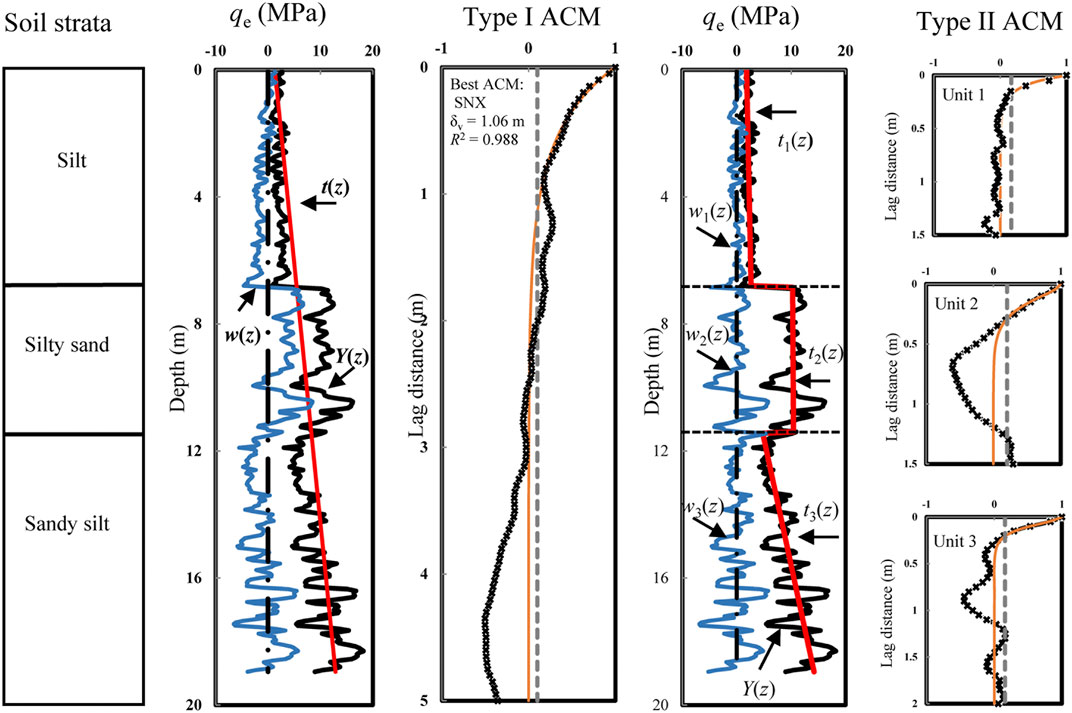
FIGURE 5. Estimation of random field parameters of the q_e profile in Case 1.

For Type I analysis, a global trend is removed and the δ_v is estimated from the corresponding fluctuation component, as shown in Figure 5. For Type II analysis, the linear trends are estimated and removed individually for three identified soil units, as shown in Figure 5. The δ_v values of three soil units are then determined by fitting ACMs respectively. The linear trend can be directly estimated using the “Trend” function in Excel. Eq. 6 indicates that under the assumption of weak stationarity, the autocorrelation coefficient at a given lag distance can be approximated by the Pearson correlation coefficient. In a soil unit, if the residuals of q_e are recorded as (w₁, w₂, … , w_n), at the jth (j = 0, 1, 2, … , n/4) lag distance, the ACF can be estimated simply using the “Pearson” function in the Excel software as “Pearson(w₁:w_n-j, w_j+1:w_n)”.

Figure 5 and Table 5 illustrate the estimated ACFs compatible with fitted ACMs for Case 1. For Type I analysis, the random field parameters of q_e along the pile shaft are μ_qe = 7,094 kPa, COV_qe1 = 0.43, δ_vqe1 = 1.06 m with the SNX model. For Type II analysis, the random field parameters of q_e of three soil units are estimated as: 1) Unit I: μ_qe1 = 2,227 kPa, COV_qe1 = 0.35, δ_vqe1 = 0.19 m with SMK model; 2) Unit II: μ_qe2 = 10,253 kPa, COV_qe2 = 0.25, δ_vqe1 = 0.26 m with CSX model; and 3) Unit III: μ_qe3 = 9,499 kPa, COV_qe3 = 0.27, δ_vqe3 = 0.24 m with the SMK model. Since the pile is 16 m in length and 0.4 m in width, the influence zone is determined ranging from 12.8 to 17.6 m in depth. The estimated ratio of q_eg to q_ea is 0.95. Assuming that the fluctuation component of q_e with a linear trend in the influence zone is stationary enough in the second-moment sense, the random field parameters of q_ea are estimated as μ_qea = 9,177 kPa and COV_qea = 0.28, δ_vqea = 0.22 m with the CSX model. The nugget effect is not observed in the curve fitting of ACM to ACF. Therefore, the random measurement errors associated with q_e measurements are neglectable in this research.

Applying the above procedure to other cases, the random field parameters of q_e can be determined for both Type I and Type II analysis, as listed in Table 5. In Type II analysis, the standard deviations (mean and COV) of q_e in different soil units are seldom similar. Hence, assuming the fluctuation component of the whole profile is stationary, perhaps over-simplified. It is reasonable to assume that q_e data from different soil units are uncorrelated because measurements in one soil unit can hardly provide information on the adjacent soil unit. The range for spatial averaging in each unit is determined as the length of the pile shaft along with the corresponding unit. Then, the reduced COVs can be obtained for all the variables and are imported to the FORM analysis.

Reliability Analysis

The Excel-based algorithm modified from Low and Tang (1997) is developed for reliability analysis to account for the variation of the correlation matrix after data transformation. Figure 6 presents the Type II analysis of Case 1. Type I analysis is similar but more simple. Basic functions for the operation of matrices are also illustrated in Figure 6. Decomposition of the correlation matrix can be achieved using the “CHOL” function in “RealStats.xlam”. “RealStats.xlam” is developed for statistical analysis using Excel and is available on the website (http://www.real-statistics.com/). The “Solver” command in Excel can be used to obtain the minimal β subjected to the constraint of limit state function by changing V or X values.

FIGURE 6

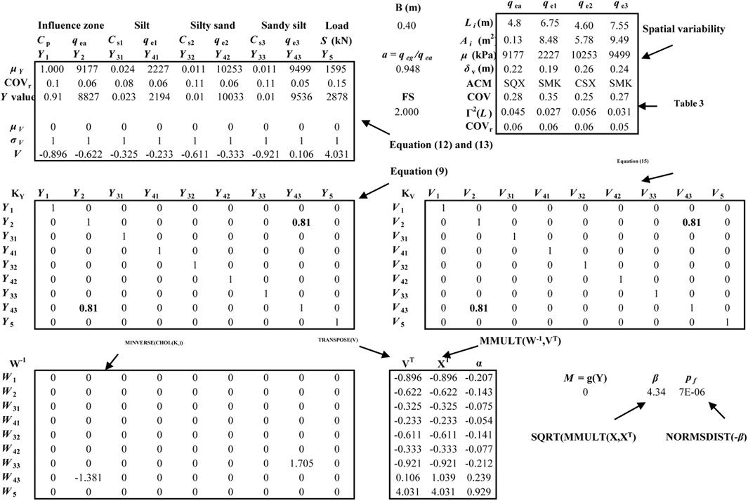
FIGURE 6. Procedure for evaluating failure probability of pile foundations (modified from Low and Tang (1997))

Discussion

For Case 1, the relationship between p_f and FS can be estimated by both Type I and Type II analysis with those parameters shown in Figure 5 and Figure 6. Similar conducts may apply to the other cases in Table 5. The results for Nanjing sites and Suqian sites are displayed in Figure 7 and Figure 8, respectively.

FIGURE 7

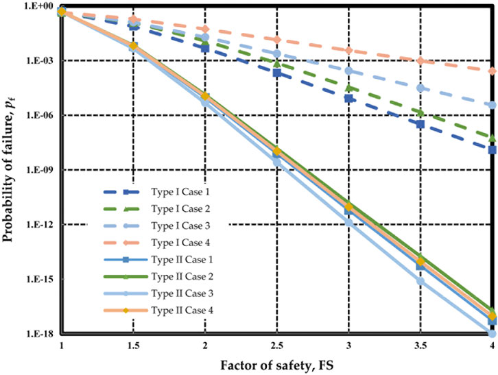
FIGURE 7. FS–P_f relationships for Nanjing sites.

FIGURE 8

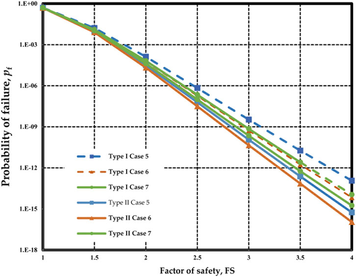
FIGURE 8. FS–P_f relationships for Suqian sites.

Effects of Spatial Variability

In Figure 7, at a small FS level, the difference between Type I and Type II is small, whereas, at a high FS level, the difference becomes conspicuous. In Case 1, when FS = 1.5, the p_f of Type I is 7.5 × 10^–2 while the p_f of Type II is 6.5 × 10^–3, the difference between the two p_f values is almost within one order of magnitude. When FS = 4.0, the p_f of Type I is 1.26 × 10⁻⁸ while the p_f of Type II is 5.3 × 10^–18. The difference between the two p_f values is about ten orders of magnitude. A similar observation is confirmed in other cases in Nanjing sites. Since all the different soil units are modeled as a homogeneous random field, the COV and δ_v can be highly overestimated. The overestimated COV and δ_v contribute to a high p_f value at the same FS level. This inference is applicable for cohesionless and cohesive soil deposits in Nanjing sites.

In Figure 8, the difference between Type I and Type II is relatively small at the same FS level. However, at a high FS level, the difference between Type I and Type II is still distinct in Case 5 to Case 7. In Case 5, when FS = 4.0, the p_f of Type I is 7.0 × 10^–12, while the p_f of Type II is 8.9 × 10^–16. However, the difference between the two p_f values is about four orders of magnitude. A similar observation is confirmed in other cases in Suqian sites.

In Case 1–Case 4, the spatial variability of geotechnical parameters in Type I is significantly different from that in Type II because the soil strata consist of different soils. In Case 5–Case 7, the means and COVs of C_s in Type I are the same as those in Type II because of the same soil strata, but the random field parameters of soils are vary greatly. In an idealized case, if the soil profile contains only one homogeneous soil unit, the reliability results of Type I and Type II are expected to be the same by the proposed framework. But even if soil strata consist of the same soil types, different interpretations of soil profiles may lead to different reliability results.

Effects of Uncertainties of Empirical Correlation Coefficients

It is of interest to investigate the impact of uncertainties of design parameters (C_p, q_ea, C_si, q_ei, S) on p_f in terms of the sensitivity factor. The design parameters are ordered according to the soil strata. Case 1 and Case 5 are studied to illustrate the influence of Type I and Type II interpretation methods on the sensitivity factors, as shown in Figure 9 and Figure 10 respectively.

FIGURE 9

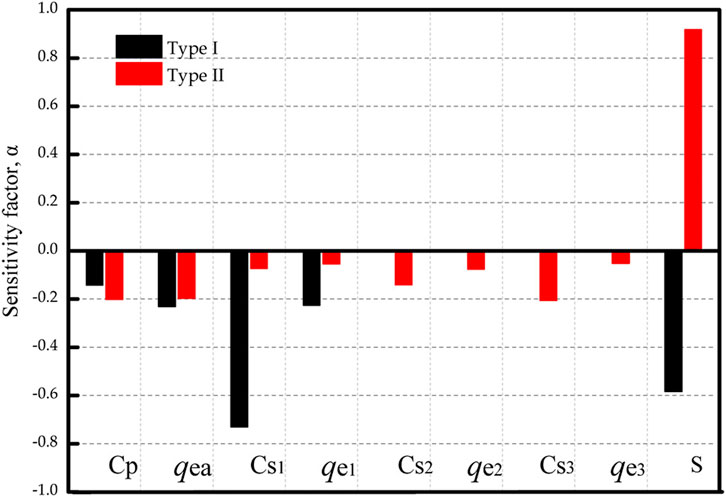
FIGURE 9. Sensitivity factors for Case 1.

FIGURE 10

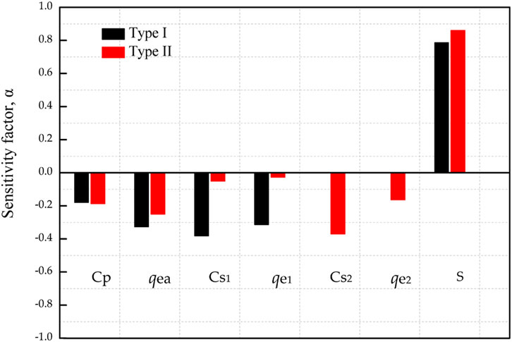
FIGURE 10. Sensitivity factors for Case 5.

For Case 1, three soil units are identified from the soil profile. In Figure 9, the p_f of Type I mainly depends on the uncertainties of the C_s and S, whereas the influences of q_ea and q_e are relatively small. During spatial averaging, the uncertainties involving q_ea and q_e are reduced, but the uncertainties of C_s are highly overestimated (COV of C_s = 0.30) in Type I. However, in Type II, the main factor influencing the failure probability is only the load, indicating that the uncertainties of the geotechnical parameters are evaluated exactly. It can be concluded that, in Type I analysis, the uncertainties of the empirical correlation coefficients will impact the failure probability significantly.

For Case 5, two soil units are identified from the whole soil profile. In Figure 10, the impact of C_s in Type I is the same as that in the Type II analysis. This can be well understood because the means and COVs of C_s are the same in Type I and Type II methods for Case 5. In Type I analysis, the absolute values of sensitivity factors of q_ea and q_e are slightly larger than those in Type II. In Type I analysis, the performance of the pile is more influenced by the uncertainties of CPTU data. This is consistent with the observation that the variability of q_e is over-estimated in Type I analysis.

A rational design can be achieved when different soil units are identified properly from the soil profile in the reliability analysis. If different soil units are not identified properly, uncertainties of CPTU data and empirical correlation coefficients should be over-estimated, the p_f may be also over-estimated, leading to a conservative design. Christian and Baecher, (2011) emphasized that over the past few decades, the failure probability of geotechnical foundations in reliability analysis is significantly overestimated, compared to the frequency of failures in practice. The failure probability of piles in layered soils can be reduced when different soil units are identified properly from a soil profile in the reliability analysis.

Conclusion

In this study, an Excel spreadsheet-based framework is developed for the uncertainty analysis of the ultimate axial bearing capacity of piles in layered soils. The uncertainty analysis is based on the UniCone direct piezocone method involving spatial variability of CPTU data and variations of empirical correlation coefficients. Proper identification of different soil units from a soil profile is crucial for estimating the failure probability of pile capacity in the reliability analysis.

The main conclusions are summarized as follows:

(1) Different interpretations of spatial variability of a soil profile may lead to different reliability results. The spatial variability of soil strata in layered soils can be evaluated accurately when different soil units are identified properly from a soil profile in the reliability analysis.

(2) For a soil profile consisting of the same soil types, the empirical correlation coefficients are the same, the spatial variability of different soil units also makes a great influence on the reliability results.

(3) As FS ranges from 1.0 to 4.0, the p_f values estimated by Type I are consistently higher than those of Type II in all cases at the same FS level, because the Type I method over-estimated uncertainties of geotechnical parameters than the Type II method.

(4) In the Type II method, uncertainties of geotechnical parameters are reduced by the proper identification of different soil units from each other in a soil profile, producing rational reliability results.

Data Availability Statement

The original contributions presented in the study are included in the article/Supplementary Material, further inquiries can be directed to the corresponding author.

Author Contributions

All authors listed have made a substantial, direct, and intellectual contribution to the work and approved it for publication.

Funding

The research was funded by the National Natural Science Foundation of China (Grant number 51908250), Program of Innovation and Entrepreneurship (Doctoral Level) of Jiangsu Province (Grant number (2020) 30537), and General University Science Research Project of Jiangsu Province (Grant number 19KJB560011).

Conflict of Interest

The authors declare that the research was conducted in the absence of any commercial or financial relationships that could be construed as a potential conflict of interest.

Publisher’s Note

All claims expressed in this article are solely those of the authors and do not necessarily represent those of their affiliated organizations, or those of the publisher, the editors, and the reviewers. Any product that may be evaluated in this article, or claim that may be made by its manufacturer, is not guaranteed or endorsed by the publisher.

References

Abu-Farsakh, M. Y., and Titi, H. H. (2004). Assessment of Direct Cone Penetration Test Methods for Predicting the Ultimate Capacity of Friction Driven Piles. J. Geotech. Geoenviron. Eng. 130 (9), 935–944. doi:10.1061/(asce)1090-0241(2004)130:9(935)

ORIGINAL RESEARCH article

Uncertainty Analysis of Axial Pile Capacity in Layered Soils by the Piezocone Penetration Test

Introduction

Uncertainties in the UniCone Method

Uncertainties of Empirical Correlation Coefficients

Uncertainties of Effective Cone Tip Resistance

The Framework of Random Field

The Scale of Fluctuation and Spatial Averaging

Coefficient of Variation

Random Field Model in Layered Soils

Correlations Among Geotechnical Parameters

Reliability Index of Pile Bearing Capacity

Reliability Analysis Theory

Data Transformation

Reliability Index

Algorithm for Reliability Index

Uncertainty Analysis of Axial Pile Capacity

Site Condition

Spatial Variability Analysis

Reliability Analysis

Discussion

Effects of Spatial Variability

Effects of Uncertainties of Empirical Correlation Coefficients

Conclusion

Data Availability Statement

Author Contributions

Funding

Conflict of Interest

Publisher’s Note

References

Glossary

This article is part of the Research Topic

People also looked at