Performance Assessment of the Cloud for Prototypical Instant Computing Approaches in Geoscientific Hazard Simulations

1 Introduction

Tsunami forecasting and hazard assessment procedures require modeling as one integral part. As an example, the accreditation of tsunami service providers in the North-East Atlantic, Mediterranean, and Connected Seas region requires model-based forecasting of tsunami hazard information (NEAMTWS, 2016).

In operational tsunami forecasting, either pre-computed scenario based hazard assessment or online simulation based approaches are common [see e.g., Behrens et al. (2010), Løvholt et al. (2019)]. Another approach—so far not operationally implemented—is statistical emulation, in which a relatively small number of true offline scenarios is used to populate a statistical interpolation (emulation) function for deriving forecasts including uncertainty values for real events (Sarri et al., 2012).

An optimal workflow for tsunami forecasting—both in near and in far field hazard forecasting—would consist of a reliable source determination followed by an integrated tsunami propagation and inundation simulation with an instant visualization and dissemination of results (Wei et al., 2013). This case would require large and scalable computing resources in case of an event for the simulation part involved in the workflow. Depending on budget and facilities, this requirement could pose unacceptable restrictions or would impose inefficient use of limited resources (since the computing resources would mostly idle, waiting for the event).

Since very flexible and large scalability is available in cloud computing environments, a straight forward strategy is to utilize the cloud for an instant computing framework for tsunami forecasting. An accepted definition for cloud computing reads (Mell and Grance, 2011):

Cloud computing is a model for enabling ubiquitous, convenient, on-demand network access to a shared pool of configurable computing resources (e.g., networks, servers, storage, applications, and services) that can be rapidly provisioned and released with minimal management effort or service provider interaction.

It is this minimal management effort and flexibility that lead scientists to explore possibilities and evaluate performance of cloud computing environments for scientific computing applications early on [e.g., Foster et al. (2009); Zhang et al. (2010); Fox (2011)].

Utilizing cloud computing environments for tsunami hazard assessment not only enables great scalability in an early warning setting, but allows for deployment of modeling capabilities to users who do not have direct access to corresponding facilities. In fact other groups have started to provide tsunami forecasting services via web services, even calling their service “cloud.” For example, the TRIDEC cloud is an online service providing simulation capabilities for tsunami forecasting (Hammitzsch, 2021). Implementing a similar workflow as the approach documented here and funded from the EU FP7 project ASTARTE, the IH-TsuSy tsunami simulation system obtains earthquake parameters from USGS, computes a tsunami wave propagation, based on corresponding sources and provides graphical information about the maximum wave height and arrival times (IH Cantabria, 2016). However, both services are strictly speaking no cloud computing efforts, since the computing devices are located at the hosting institute’s premises. A server, available to the public and capable of instantly computing tsunami scenarios, however manually triggered, is the TAT server, maintained by the Joint Research Center of the European Commission in Ispra (European Commission, 2022 Security and Migration Directorate—JRC Ispra Site). The services are provided by web interfaces and as such could be considered as a so-called platform as a service (PaaS) model. These services are not configurable and call for provider interaction to be used.

Other possible cloud computing utilization for geoscientific applications are possible and will be further discussed in the next section. This report aims at assessing performance and feasibility of cloud computing in particular for tsunami hazard modeling. The service accessed in the cloud is a so-called infrastructure as a service (IaaS) model. We document a preliminary assessment of computational performance for scientific computing on two of the major cloud computing platforms, i.e., the Amazon Web Services (AWS) and Microsoft Azure. Additionally, a prototypical implementation of an early warning modeling framework, using a Python script for controlling the workflow and utilizing Amazon Web Services (AWS) cloud computing facilities is described. The prototype demonstrates the ease of use and cost effectiveness of such cloud computing environments for online tsunami forecasting simulations. We stress, however, that the demonstrator is by far not fit for operational services, since more optimization of the tsunami model, more fine-tuning of the required data, quality control, and testing would be necessary, which is outside of the scope of this study.

2 Motivation

As described in the introduction (Section 1), one of the main motivations for an instant computing framework using cloud instances is to perform online tsunami forecast simulations efficiently and reliably in the event of a tsunamogenic earthquake. This section intends to motivate the use of such facilities in some more detail and strives to assess the strengths and weaknesses of the approach.

One of the first motivations for using the cloud for tsunami modeling in case of early warning use cases was the cost effectiveness of cloud computing. In fact, an hour of CPU time on a reasonably sized cloud device costs approximately 2.00 USD. This includes investment, energy, cooling, maintenance and administration, as well as utility costs and needs to be spent only if used. Some additional costs are to be allocated for storage and network traffic, however this is very difficult to assess, since it depends very much on the actual situation and usage. Therefore, we will compare very coarse estimates in the following. We are aware of the preliminary character of this assessment, but think it is nevertheless useful as a guiding example.

Let us compare a cloud computing approach to on-premise computing for a usual deprecation period (for computing hardware) of 3 years and let us assume a (relatively high) number of processed tsunami events of 50 per year (or roughly 1 per week). In the cloud, every event needs computing time, so we assume approx. ten aggregated CPU hours of computing time per event. An appropriate medium size general purpose Amazon EC2 instance of 32 vCPUs (virtual CPUs), 128 GB of RAM and approx. 1,000 GB SSD intermediate storage costs (e.g., m5.8xlarge¹) approx. 2.00 USD per hour or 20.00 USD per event, totaling to 3,000.00 USD over the period of 3 years. The same applies to an Azure D32 v3 instance², comprising also 32 CPUs, 128 GB of RAM, and 800 GB of local storage. We might need to add some cost for implementation and testing, but since this can be done on smaller instances, the cost should not exceed approx. 1,000.00 USD. Furthermore, we assume approx. 50.00 USD per month for storage and data transfer, amounting to a total of 1,800.00 USD over the period of 3 years.

For the on-premise cost comparison we assume a reasonable server of 64 GB main memory, similar number of cores as for the cloud instances (e.g., 4 nodes of 8 cores each), and an appropriate hard drive installation totaling an investment of approximately 10,000.00 USD. Furthermore, such device consumes approx. one kilo Watt of electrical power per hour and we assume the cost for energy with 20 cents per kWh. Furthermore, we need to provide cooling, which we have assumed of the same order as the energy costs. Maintenance can be achieved by assuming one 10th of a full time equivalent of a technician, costing approx. 7,500 USD per year. We neglect utility costs and costs for repairs for now. A summary of these estimations can be found in Table 1. All in all, the cost for on-premise computing can be estimated with 42,900.00 USD versus costs for on-demand cloud computing of 5,800.00 USD. We repeat at this point that these numbers are very preliminary and may vary substantially with location, since labor costs as well as energy costs are quite different in different parts of the world.

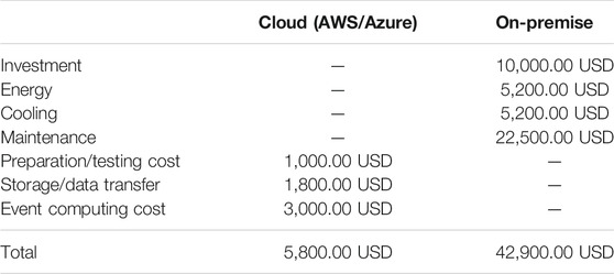
TABLE 1. Cost comparison of cloud and on-premise computing.

An important argument for keeping computing facilities on-premise is the availability. In order to have a redundant computing environment that is fail-save in case of emergency, two computing devices would be necessary and in principle, these should be maintained at different locations. With cloud computing devices, the location can be everywhere. The above mentioned Amazon EC2 instance is available in more than 20 locations worldwide on all continents (except Antarctica). The service level agreement of the Amazon EC2 guarantees 99.95% availability for one of the locations. When assuming (as stated in the agreement) a month of 30 days, the system may fail for up to 21 min. However, in this case yet another of the locations could be reached. It is hard to achieve such low failure rate with an on-premise service, in particular in less developed areas.

Of course, a communication network needs to be in place. But again, it can readily be argued that in times of abundant redundant mobile communication networks, establishing a communication to a cloud server might be more reliable than an on-premise solution. Even in case of failed local communication, ad-hoc peer-to-peer networks of mobile devices are ready to be established (ASTARTE Project, 2017b).

One particular advantage of a cloud computing solution is its accessibility from everywhere. Even in remote areas, where maintaining compute infrastructures may not be feasible, a communication (e.g., via satellite link) to a cloud computing device could be established and would allow for scalable modern computing capabilities. Additionally, the cloud instance can be accessed from mobile devices.

Since the cloud infrastructure is easily scalable, it is possible to run several computations in parallel. A common practice in numerical weather forecasting—namely ensemble forecasts—could be established in tsunami modeling for capturing the uncertainty and quantifying it by varying the source parameters (Selva et al., 2021).

Access to the cloud infrastructure works with web interfaces and secure shell access. Web interfaces are used to start, control, and stop the cloud instance, which in our demonstration cases are always stored as virtual Linux machines. While the cloud instance is not running, storage of these several tens of gigabyte large files generates costs of the order of a few dollars per month. The virtual machine is pre-configured with compiled versions of the simulation code, repositories for bathymetry and topography data, post-processing tools, and possibly visualization pipelines. In the presented prototype, the sources are computed from moment tensor solutions available by web service from the GEOFON web page (GEOFON, 2021). Bathymetry and topography data are prepared and stored in the virtual machine, but could potentially also be retrieved on demand. In our case, visualization is performed on a local personal computer, but it would also be possible to configure a second cloud instance especially dedicated for high-performance visualization such that the results can readily be obtained by mobile devices such as smart phones or public projection screens.

Looking beyond hazard computing, cloud computing enables researchers and institutions without funding for large investments access to large scale computing facilities. Since cloud computing instances can be tailored and scaled to the requirements during development and production phases on demand, cost efficiency can be achieved and large computations are accessible with low budgets. Even in research environments, where larger budgets are generally available, it may be difficult to allocate investments into large computing infrastructures. In that case cloud computing costs can be accounted to research project material expenses and do not necessitate any investments.

Another important advantage goes beyond the application of tsunami hazard assessment. The cost efficient availability of cloud computing infrastructure would allow countries without locally available large-scale computing resources to run local hazard assessments in case of, e.g., potentially severe weather events where devastating effects of such events have greater human impact than in industrial countries with advanced computing and warning infrastructure that run their own weather services.

Last but not least, large on-premise computing hardware has a significant disadvantage in countries, where energy costs are high, such as in central Europe or in very warm countries. An enormous amount of energy is required for cooling. Cloud computing hardware can be placed anywhere. As an example, in Iceland cloud computing facilities can be run and cooled using geothermal energy only. Thus the impact of running cloud computing hardware on the environment can be minimized in contrast to on-premise solutions.

3 Performance Assessment

In order to assess the feasibility of large scale geoscientific computing in cloud infrastructures, we perform benchmark tests representing numerical operations typically occurring in applications such as tsunami simulations, shown in the next section, as well as other geoscientific applications with high computational demands. We employ different sets of benchmarks in different cloud computing environments. Our tests were performed on the AWS cloud, employing a Fortran program for solving an elliptic partial differential equation by classical iteration, parallelized alternatively with OpenMP or MPI. These tests were performed in a comparison with an on-premise computer in the context of the ASTARTE project (ASTARTE Project, 2017a) and documented in an internal report. They are reported here for reference and for a better comparison and understanding.

The second set of benchmarks is performed using a mixed OpenMP-MPI parallelized C/C++ implementation of advection-diffusion type partial differential equations. These types of equations are typical for all kinds of geoscientific phenomena and are often used as a first representation for the development of numerical algorithms in this application field. Tsunamis can be represented by a non-linear generalization of such equation type. This benchmark will be tested on a number of differently sized instances of the Azure cloud computing platform.

3.1 Description of Elliptic PDE Benchmark—AWS Cloud

The elliptic partial differential equation solved in this benchmark represents a simple Poisson equation in two spatial dimensions:

We use f (x, y) = 2 (x + y − x² − y²) and g ≡ 0. $u(x,y)\in \mathbb{R}$ is an unknown potential. The domain Ω is discretized by a uniform equidistant grid (x_i, y_j) = (iΔx, jΔx), with $\mathrm{\Delta }x=\frac{1}{n}$, i, j = 0: n, of (n + 1) × (n + 1) grid points, and δΩ is the boundary of Ω. Discretizing this equation by a finite difference operator and solving by an iterative Gauß-Seidel procedure results in an inner loop operation of the form

where u (i, j) = u (x_i, y_j), and k represents the iteration count. The discrete form requires an access pattern to the nearest neighbors. When ordering the grid points in a white-black checkerboard pattern, the white and the black points can be processed in parallel and only one barrier synchronization is necessary within each iteration. The access pattern is visualized in Figure 1. The unknowns are distributed to processors in equal sized areas with full columns. Each processor has read access to one column to the left and right of its own domain, so that after each iteration these rows need to be communicated among neighbors, when local memory message passing (MPI) is employed. Computation of white nodes and black nodes is completely independent and could also be distributed in a different way. Within each iteration a synchronization is necessary, when switching from black to white nodes. A five point stencil is marked for the access pattern in Equation 1.

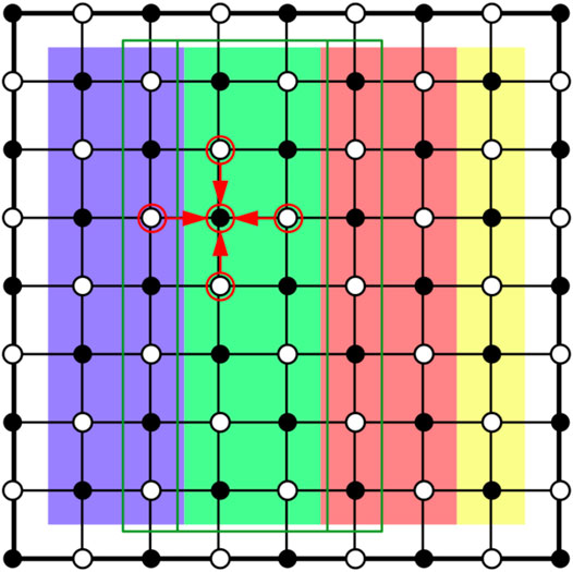
FIGURE 1. Access pattern and domain decomposition of the red-black relaxation method used in the algorithm for performance testing in Section 3.1. Underlying colors indicate the distribution to processors, only interior nodes are processed. The access stencil is indicated by arrows. Green lines indicate the region, where read access to neighboring nodes is necessary.

3.2 Description of Elliptic PDE Benchmark—Azure Cloud

The same model as in Section 3.1 is tested in Microsoft’s Azure cloud environment with a modified right hand side:

It is a modified version of an example within the Deal.II library (“step 40”). We solve the model using a computationally more demanding adaptive finite element method (FEM) in 2D on a distributed mesh with parallel linear algebra. The solver is implemented using the Deal.II library (Arndt et al., 2020).

Essentially, this is the same test case that has been conducted in Bangerth et al. (2012) on an on-site high-performance cluster to show the scalability of certain functionality within Deal.II whereas we exploit this well tested high-performance computing software to show the suitability of scalable cloud environments. Note that the right-hand side constitutes a discontinuous forcing. This causes the solution to display large gradients at the discontinuity and hence the mesh is expected to be refined there allowing us to test the performance in a sequence of refinement cycles that constitute different problem sizes. The test is conducted on two cluster settings:

3.2.1 Small Setup

This setup consists of a small sized master node that does not participate in the actual computation but serves as a load balancer running a SLURM scheduler (Yoo et al., 2003). This master node distributes the MPI-parallel computation across ten compute nodes each equipped with an Intel^® Xeon^® Platinum 8272CL, 2.1 GHz, with 2 cores and 8 GB of RAM. This is also the setup for the master node. The nodes are connected in a fast and modern Infiniband network which facilitates a high communication throughput. A shared SSD data storage of 256 GB was mounted on each of the compute nodes.

3.2.2 Large Setup

The same load balancer as in the small setup is reused with ten compute nodes each equipped with an Intel^® Xeon^® Platinum 8168, 3.4 GHz, with 32 CPU cores (16 physical and 16 virtual) and 64 GB of fast main memory.

3.3 Description of Bouyancy-Boussinesq PDE Benchmark

This test case is the basis for the large scale framework ASPECT (Bangerth et al., 2015) that serves the purpose of the simulation of convection processes inside the earth mantle. As in Section 3.2 we run it with essentially the same parameter configuration as in Bangerth et al. (2012) but yet, again, to demonstrate the feasibility of well tested high performace software for cloud computations. The model is essentially a temperature feedback driven incompressible Stokes model with an advection-diffusion equation for the temperature variable. The model equations are given by

Here, u is the velocity, T the temperature, p the pressure, ρ a density, μ is a thermal conductivity of the medium, ϵ ist the symmetric gradient (strain), g the gravitational constant, e_r the outward normal vector, $T_{\mathsf{ref}}$ and ${\rho }_{\mathsf{ref}}$ reference temperature and density, respectively. The implementation uses H¹-conformal linear finite elements for velocity and temperature and L²-conformal (discontinuous) elements for the pressure and is again a modified version of an example of the Deal.II library (“step 32”).

3.4 AWS Benchmark Results

While the elliptic test problem does not cover all different computational aspects of a tsunami simulation—in particular not with the discontinuous Galerkin approach, used in the prototypical implementation in Section 4—it is suited to give a good first impression of the computational capabilities of cloud instances in real life application scenarios. In order to assess the expected performance of a cloud instance in comparison with an on-premise compute server tests with up to 8 processors are conducted. It turns out that the test program does not scale very well, but it is not the purpose of this test to see optimal parallel performance but to be able to compare cloud vs. on-premise computing devices. Parallelization is implemented by the Message Passing Interface (MPI) parallel programming model, and no specific action is taken to optimize parallel efficiency. Note that these tests were performed some time ago and are included in this report for reference.

The tests are performed with the following configurations. The on-premise computer is a 2 node 2.67 GHz Xeon X5650 server with 12 cores, which is used with up to 16 processes (hyperthreading). It is equipped with 32 GB of main memory. The AWS EC2 cloud instances are of type c3.8xlarge, which is a Xeon E5-2680 based architecture with 32 virtual processors, 60 GB of main memory, and 10 GBit high speed networking. The performance results are shown in Figure 2. It can be seen from the figure that the local on-premise computation is a factor of 2 slower due to different processor generations, but the parallel scaling shows approximately the same behavior for the cloud as well as for the on-premise servers.

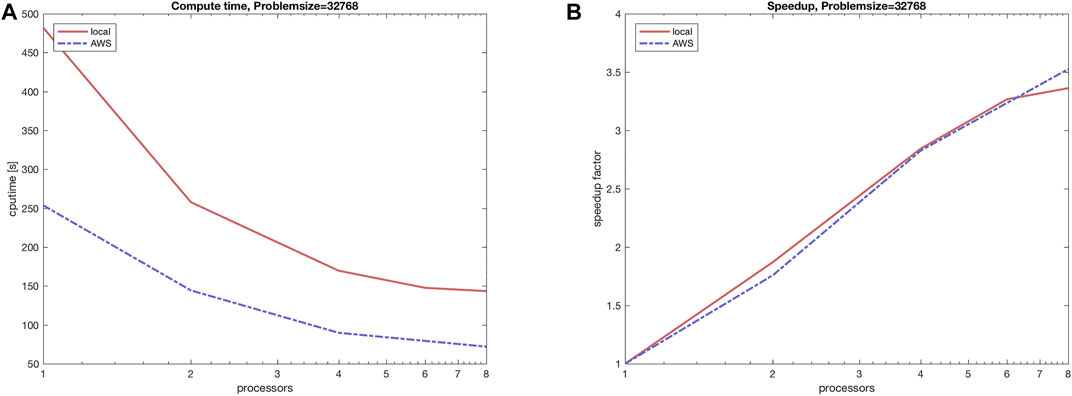
FIGURE 2. (A) Compute time comparison for parallel execution of benchmark program in Section 3.1 on an on-premise computer in comparison with AWS EC2 cloud instances. (B) The speedup (strong scaling) of the corresponding benchmark tests.

As a preliminary conclusion, it can be stated that the same kind of performance can be expected from an on-premise server as well as from a cloud instance. Performance-wise there is no specific advantage using an on-premise computer. In particular looking at the cost comparison of the previous chapter 2, the cloud instance can be regarded as the advantageous architecture.

3.5 Azure Benchmark Results

3.5.1 Elliptic PDE Benchmark

We perform weak and strong scaling tests, i.e., we take timings with fixed allocated hardware and gradually increase the problem size (weak scaling) as well as timing tests, where we fix the problem size and gradually allocate more compute resources (strong scaling). Both scaling tests are performed on the small and the large setup as described in Section 3.2. Although both our small and large setup are rather small compared to the cluster setup used in Bangerth et al. (2012), allowing only qualitative comparisons, similar (linear) scaling effects for differently sized problems are clearly visible for weak and strong scaling, see Figure 3. The scaling tests show timings of the main building blocks of adaptive FEMs which are essentially the setup of the mesh and the distribution of the degrees of freedom (dof setup), the assembly of the (sparse) system (assembly), the conjugate gradient solver preconditioned with algebraic multigrid (solver), a posteriori error estimation and adaptive coarsening and refinement of the mesh including rebalancing the mesh (coarsen/refine), and the data output (output). Figure 4 additionally shows the partitioning of the adaptive mesh among 20 MPI processes.

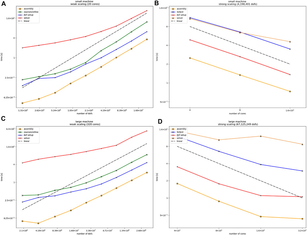
FIGURE 3. (A) Weak scaling in the small setup for the test case in Section 3.2 computed on 20 distributed CPUs with up to 17 million degrees of freedom. (B) Strong scaling for selected parts of the algorithm for the small setup with 4.2 million degrees of freedom on up to 16 distributed cores. (C) Weak scaling in the large setup for the test case in Section 3.2 computed on 320 distributed CPUs with up to 270 million degrees of freedom. (D) Strong scaling for the large setup with 67 million degrees of freedom on up to 320 distributed cores. Both weak scaling plots do not show timings for the data output since its overhead becomes dominant at around 10⁸ Dofs. Both strong scaling plots do not time coarsening and refinement since the runs are not adaptive.

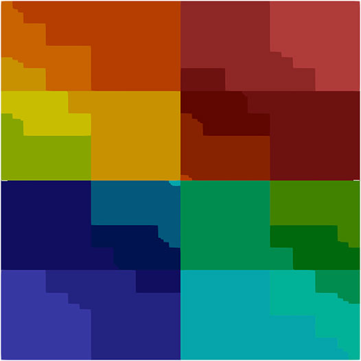
FIGURE 4. Distributed mesh (20 CPUs on 10 nodes, small setup) for the test case in Section 3.2. Each color indicates a different processor owning a part of the mesh.

Remark. We pass on timing the output in the weak scaling tests Figures 3A,C in our parallel setting since its overhead becomes very dominant for problem sizes with a number of degrees of freedom at a magnitude 10⁸ and higher and simply does not fit nicely in the plot of (Figure 3C). Also, Figures 3B,D do not show timings of refinement and coarsening, because it was disabled for the strong scaling setup since we used a fixed number of degrees of freedom and only increased the number of processors.

3.5.2 Bouyancy-Boussinesq PDE Benchmark

This is an example of a massively parallel implementation since idle cores on each node will also be used for local shared memory parallelism. Thus for a substantial test of strong scalability taking full control over local threading and carefully choosing the balance of participating compute nodes versus the number of local cores on each node and the accessibility of memory banks is necessary. We pass on this and only show weak scaling results on 160 CPU cores on all ten machines. Note that the remaining virtual cores are used for threading the assembly of the system matrices and right-hand sides. Also note that we do not scale to the same large number of DoFs as in the test of Section 3.2 since the problem is numerically much more challenging. Figure 5 shows a snapshot of the Bouyancy-Boussinesq problem applied to mantle convection applications. Figure 6 shows the weak scaling effects on 160 cores in the large setup for 100 time steps and increasing problem sizes due to adaptive mesh refinement. Note that coarsening and refinement includes re-balancing the mesh, and that the solvers scale slightly better than linearly since the solution at the preceding time step is used as an initial guess. The overall solution times for each iteration show slightly better scaling than linear, most likely because we are not in the asymptotic regime.

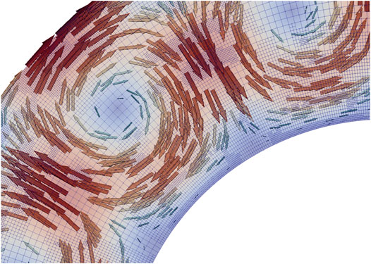
FIGURE 5. Snapshot of the solution of the Boussinesq test case of Section 3.3. A crossection of the earth’s mantle is shown with the adaptively refined mesh. Arrows indicate the flow direction and speed. Color also indicates flow speed.

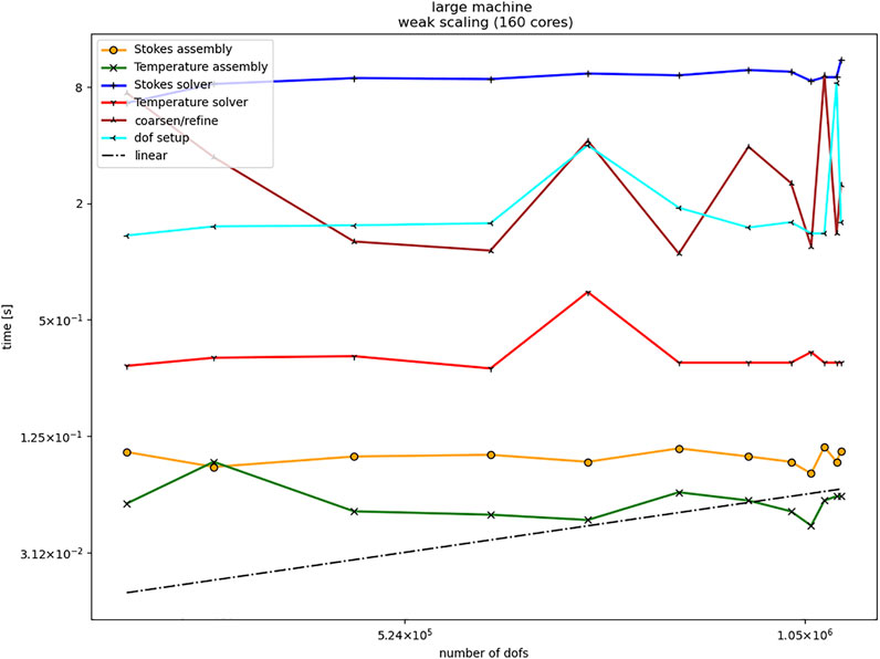
FIGURE 6. Weak scaling on 160 CPU cores with local threading on ten nodes for the test in Section 3.3 (large setup).

Overall, these scaling examples demonstrate the capacity of cloud facilities for typical numerical computation primitives. Scaling as well as absolute performance indicators are similar to on-premise computing facilities, at least for reasonably sized computers. The software environments of cloud instances are very similar to on-premise computing facilities, since the cloud instances can be configured analogously, providing Linux operating systems with the usual libraries and compilers, and even specialized libraries can be installed into the virtual machines running in the cloud environments.

4 Example Workflow for Tsunami Hazard Computing

A prototypical workflow for an instant computing scenario in tsunami early warning could be given by the following sequence:

1. Trigger: Earthquake detected through network of seismometers and suitable processing, information available via web service [e.g., GEOFON (2021)]

2. Gather Boundary Data: Bathymetry/topography data (possibly pre-) processed from online resources for the computational domain of interest.

3. Derive Initial Data: Obtain rupture parameters (Okada parameters) from earthquake parameters, e.g., through scaling laws (Mansinha and Smylie, 1971; Okada, 1985; Kanamori and Brodsky, 2004).

4. Simulation: Run tsunami forecasting simulation with initial conditions (Okada) and boundary data from previous two steps.

5. Deploy/visualize results: Visualize simulation results, and deploy additional products through web services from data, which were generated and stored in files during the simulation.

This workflow is given in Figure 7 as a flow diagram.

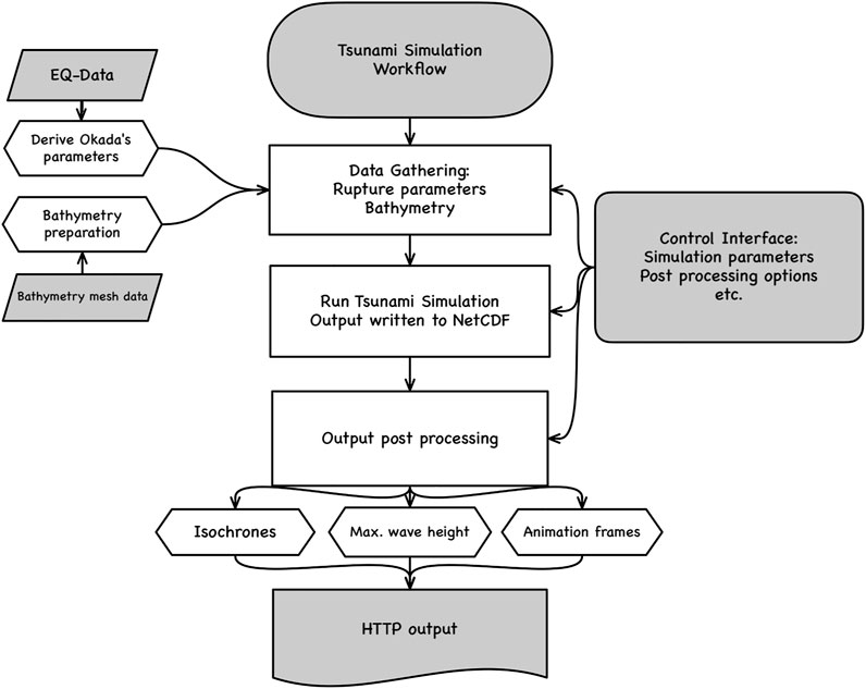
FIGURE 7. Prototypical workflow for tsunami forecasting.

In order to implement a prototypical realization of this workflow, several pre-fabricated tools were available and have been used. As a first step, however, a well configured AWS EC2 virtual machine instance needs to be generated. Since the EC2 instances are scalable, the configuration concerns in particular the connectivity of the cloud machine. In our case access to the machine is established via secure shell (SSH) on port 22, and the (secure) HTTP/HTTPS protocols via ports 80 and 443 respectively. Corresponding keys need to be generated and stored appropriately.

The workflow is implemented by a 250 line Python script. In order to be able to achieve this brevity, several pre-fabricated libraries are used. The Boto library (Amazon Web Services, 2021) helps to start and configure the EC2 instance out of the python run-time environment. To simplify the interaction with the EC2 instance via SSH the Paramico library (Forcier, 2021) is used.

The general architecture of the implementation is shown in Figure 8. The Python controller script can run either on a very small/weak cloud instance or on any computer on-premise. It uses hardly any resources and will just listen to incoming mail from the triggering earthquake alert service. When the workflow is triggered by an earthquake alert message, the controller starts the EC2 instance, which is stored as a pre-fabricated and configured virtual machine. This consists of a current Debian Linux operating system, a repository of bathymetry/topography data for the region of interest (in our case the western Mediterranean), a compiled simulation program (StormFlash2d, see below) with all necessary libraries, and post-processing tools. Once the EC2 instance is running, it provides an HTTP-interface for clients, including mobile devices, to retrieve simulation results.

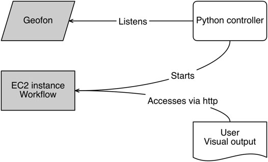
FIGURE 8. Architecture of the prototypical cloud based tsunami forecasting system.

In this prototypical implementation the trigger for activating the workflow is an email sent by the GEOFON server (GEOFON, 2021) in case of an earthquake. The alerting email contains information on the earthquake’s epicenter location, time, source parameters, and a unique event identifier. For reasonably significant earthquakes moment tensor parameters are automatically computed and can be accessed via web interfaces. The python controller parses relevant values from the text file containing the moment tensor parameters and derives the corresponding input to be used in the Okada model for tsunami sources (Okada, 1985). The empirical formulas are taken from Pranowo (2010) and are based on Kanamori and Brodsky (2004); Mansinha and Smylie (1971) and others.

Once the Okada parameters are derived, the corresponding source serves as initial condition for starting the simulation. Other boundary conditions (bathymetry/topography) are obtained from previously prepared and stored data. The propagation and inundation is computed by the simulation software StormFlash2D, an adaptive discontinuous Galerkin non-linear shallow water model (Vater et al., 2015, 2019). The output of StormFlash2D—wave height and velocity on adaptively refined triangular meshes—is stored in NetCDF files (Unidata, 2021), following the UGRID conventions (Jagers, 2018). These files are then further processed and visualized, utilizing the pyugrid Python library (Barker et al., 2021). Post-processing can then be applied to the stored files, in order to derive forecasting products, such as arrival time maps, mareograms, etc.

In this prototypical implementation that serves mainly the purpose of demonstrating feasibility, we use parameters similar to the 2003 Zemmouri-Bourmedes tsunami event at the coast of Algeria in the Mediterranean (Alasset et al., 2006). The example email triggering the workflow contains the earthquake magnitude (MW 6.8) and location data (epicenter 36.83 N, 3.65 E, and depth 8 km). Further local tensor data are assumed to be strike 54°, dip 50° and rake 90°. Applying the above mentioned empirical scaling laws to the earthquake magnitude, we set a slip of little less than 1 m, a length of the Okada plate of 30.2 km and a width of 15.1 km. A single plate is assumed.

The only product delivered to a potential user in this feasibility study is a short animation of waves propagating over the ocean area of interest (see Figure 9). This sequence is computed using standard gebco bathymetry GEBCO (2014), which is interpolated linearly to the triangular mesh. The mesh for this computation was not adapted, but used in a uniformly refined version with 16 refinement levels, corresponding to a grid of approx. 260,000 grid cells or to a resolution of approx. 1,300 m. Note that in the visualization, there are some numerical artifacts (secondary waves) caused by a somewhat sloppy implementation of the interpolation of the Okada initial conditions (computed on a rectangular mesh) to the triangular computational mesh of StormFlash2d.

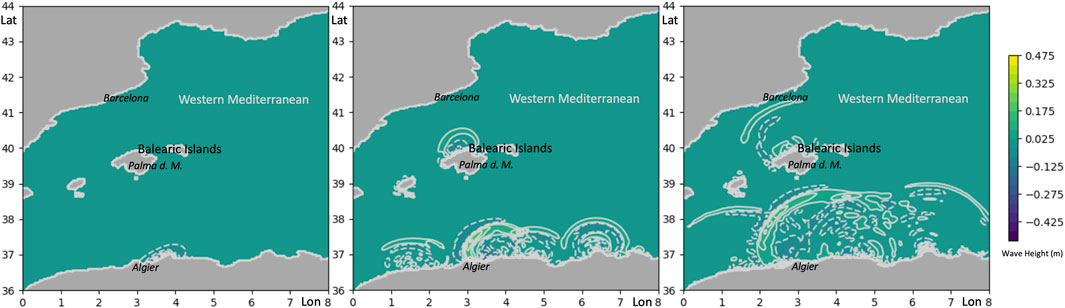
FIGURE 9. Three snapshots of an animation result from the prototypical cloud based tsunami simulation. x- and y-axis represent degrees East longitude and North latitude, colors/contour lines indicate wave amplitude in meters. This is a scenario with a synthetic source of an earthquake tsunami originating in the North Algerian subduction zone. The images cover a map area reaching from approximately Valencia/Spain in the West to Monaco in the East and from a little South of Algier/Algeria in the South to Montpellier/France in the North.

The above steps, i.e., listening to incoming email, parsing data into files controlling the execution of the tsunami model, and collecting output data, are performed by a small Python script on a local laptop or desktop computer. Starting the EC2 AWS instance takes less than 30 s. Run time for this serial computation on one node of the AWS instance takes approx. 100 s, the time for output being less than 1% of the total computing time.

While this proves the feasibility of implementing such workflow in IaaS type cloud services, it is by no means useful for real world operations. The adaptive tsunami simulation—while potentially efficient and accurate—is not applied to local resolutions of 10 s of meters for usefully precise forecast information. If this was the aim, additional resources and performance optimizations would be necessary. Additionally, a more diverse and more quality controlled post-processing pipeline would be necessary. Usually, wave arrival time maps, wave height maps, possibly inundation maps, and even flow speed assessments would be of practical interest.

5 Summary and Conclusion

In this study we assess the feasibility of on-demand cloud computing for tsunami hazard assessment as well as other demanding geophysical applications. On the one hand, we test the capacity of cloud computing environments to provide scalable high-performance computing capabilities. A number of advantages of such cloud-based computing facilities motivate us to further investigate their usability for more practical applications. Therefore, we propose a simple workflow that can be implemented in a cloud environment. While we are aware that there exist similar workflows in tsunami hazard assessment, they are all based on remotely accessible, but local on-premise computing environments.

A simplified prototypical workflow, utilizing cloud instances is implemented and demonstrates the overall feasibility of our approach. More work needs to be invested to empower this approach for operational use:

• Some manual work is required to obtain quality controlled bathymetry/topography data.

• A permanent control process needs to be instantiated in order to listen to relevant trigger data (such as earthquake portals) and compute robust and useful sources from earthquake parameters. The prototypical application is much too simple for operational purposes.

• More relevant output formats and better visualization needs to be implemented to interact with the instant computing workflow.

• The simulation software StormFlash2D needs thorough parallelization and optimization to be used in an operational environment.

• It would be desirable to also include other operational models for assessing the uncertainty in the forecast, related to the modeling technique.

• Instantiating several on-demand computations with a variation in the earthquake parameters within the data uncertainty, would create an ensemble of forecasts, allowing for probabilistic forecasts such as those proposed by Selva et al. (2021).

By conducting the scalability tests with selected benchmarks we could show that cloud computing environments are capable of providing the required performance for many geoscientific applications at reasonable costs. Therefore further exploration and development of standardized interfaces for managing and controlling the cloud computing infrastructure is worthwhile.

Data Availability Statement

The raw data supporting the conclusion of this article will be made available by the authors, without undue reservation.

Author Contributions

JB wrote main parts of the article, coordinated the project, and raised funding. AS provided and configured the necessary cloud infrastructure, and performed early benchmark tests on the AWS cloud. KS configured the software environment and ran most of the tests in the Azure cloud.

Funding

Parts of this research were conducted in the framework of the ASTARTE project with funding from the European Unions Seventh Program for research, technological development and demonstration under grant agreement No. 603839. Additional funding was obtained by the Deutsche Forschungsgemeinschaft (DFG, German Research Foundation) under Germany’s Excellence Strategy—EXC 2037 ’CLICCS—Climate, Climatic Change, and Society’—Project Number: 390683824, contribution to the Center for Earth System Research and Sustainability (CEN) of Universität Hamburg.

Conflict of Interest

Author AS was employed by the Axtrion GmbH & Co. KG.

The remaining authors declare that the research was conducted in the absence of any commercial or financial relationships that could be construed as a potential conflict of interest.

The handling Editor declared a past co-authorship with the authors JB.

Publisher’s Note

All claims expressed in this article are solely those of the authors and do not necessarily represent those of their affiliated organizations, or those of the publisher, the editors and the reviewers. Any product that may be evaluated in this article, or claim that may be made by its manufacturer, is not guaranteed or endorsed by the publisher.

Acknowledgments

The authors gratefully acknowledge the following individual contributions. Development of the tsunami demonstrator was mainly conducted by JB’s student Mathias Widok, who implemented the Python code and configured AWS instances for the demonstrator application. Stefan Vater, post-doc in JB’s research group, together with Michel Bänsch, student assistant, provided the tsunami simulation software StormFlash2D and configured it to be used in the western Mediterranean. Assistance in benchmarking and performance assessment of the benchmark AWS cloud instances was provided by the Andreas Oetken for Axtrion.

Footnotes

¹According to https://aws.amazon.com/de/ec2/pricing/on-demand/, last accessed 2022-01-21.

²According to https://azure.microsoft.com/de-de/pricing/calculator/, last accessed 2022-01-21.

References

Alasset, P.-J., Hébert, H., Maouche, S., Calbini, V., and Meghraoui, M. (2006). The Tsunami Induced by the 2003 Zemmouri Earthquake (Mw= 6.9, Algeria): Modelling and Results. Geophys. J. Int. 166, 213–226. doi:10.1111/j.1365-246x.2006.02912.x
Amazon Web Services (2021). Boto 3 Docs 1.17.53 Documentation. Available at: https://boto3.readthedocs.io/en/latest/. Accessed: 2021--04-18.
Arndt, D., Bangerth, W., Blais, B., Clevenger, T. C., Fehling, M., Grayver, A. V., et al. (2020). The deal.II Library, Version 9.2. J. Numer. Maths. 28, 131–146. doi:10.1515/jnma-2020-0043
ASTARTE Project (2017a). Assessment, Strategy and Risk Reduction for Tsunamis in Europe. Available at: https://cordis.europa.eu/project/id/603839/reporting. Accessed: 2022-02-04.
ASTARTE Project (2017b). Find platform, fundação da faculdade de ciências da universidade de lisboa. Available at: http://accessible-serv.lasige.di.fc.ul.pt/∼find/. Accessed: 2017-05-13.
Bangerth, W., Burstedde, C., Heister, T., and Kronbichler, M. (2012). Algorithms and Data Structures for Massively Parallel Generic Adaptive Finite Element Codes. ACM Trans. Math. Softw. (Toms) 38, 1–28.
Bangerth, W., Dannberg, J., Fraters, M., Gassmoeller, R., Glerum, A., Heister, T., et al. (2015). Aspect v1.5.0: Advanced Solver for Problems in Earth’s Convection. Comput. Infrastructure Geodynamics. doi:10.5281/zenodo.344623
Barker, C., Calloway, C., and Signell, R. (2021). Pyugrid 0.3.1: A Package for Working with Triangular Unstructured Grids, and the Data on Them. Available at: https://pypi.python.org/pypi/pyugrid. Accessed: 2021-06-27
Behrens, J., Androsov, A., Babeyko, A. Y., Harig, S., Klaschka, F., and Mentrup, L. (2010). A New Multi-Sensor Approach to Simulation Assisted Tsunami Early Warning. Nat. Hazards Earth Syst. Sci. 10, 1085–1100. doi:10.5194/nhess-10-1085-2010
European Commission (2022). Space, Security and Migration Directorate - JRC Ispra Site. Tsunami analysis tool (tat) Available at: https://webcritech.jrc.ec.europa.eu/TATNew_web/ (Accessed 01, 19).2022.
Forcier, J. (2021). Paramico - a python Implementation of Sshv2. Available at: http://docs.paramiko.org/en/2.1/. Accessed: 2021-06-27.
Foster, I., Zhao, Y., Raicu, I., and Lu, S. (2008). Cloud Computing and Grid Computing 360-degree Compared. IEEE Xplore. doi:10.1109/GCE.2008.4738445
Fox, A. (2011). Cloud Computing-What's in it for Me as a Scientist? Science 331, 406–407. doi:10.1126/science.1198981
GEBCO (2014). The Gebco_2014 Grid, version 20150318.Available at: https://www.gebco.net. Accessed: 2022-01-19.
GEOFON (2021). Geofon Homepage. Available at: http://geofon.gfz-potsdam.de. Accessed: 2021-06-27.
Hammitzsch, M. (2021). Tridec Cloud for Tsunamis, Gfz German Research center for Geosciences. Available at: http://trideccloud.gfz-potsdam.de/. Accessed: 2021-06-27.
Cantabria, I. H. (2016). Ih-tsunamis System (Ihtsusy) an Online Real-Time Tsunami Simulation and Notification Application. Available at: https://ihcantabria.com/en/specialized-software/ih-tsusy/. Accessed: 2021-06-27.
Jagers, B. (2018). Ugrid Conventions (v1.0). Available at: http://ugrid-conventions.github.io/ugrid-conventions/. Accessed: 2021-06-27.
Kanamori, H., and Brodsky, E. E. (2004). The Physics of Earthquakes. Rep. Prog. Phys. 67, 1429–1496. doi:10.1088/0034-4885/67/8/r03
Lovholt, F., Lorito, S., Macias, J., Volpe, M., Selva, J., and Gibbons, S. (2019). “Urgent Tsunami Computing,” in IEEE/ACM HPC for Urgent Decision Making (UrgentHPC) (Denver, CO; USA: IEEE), 45–50. doi:10.1109/UrgentHPC49580.2019.00011
Mansinha, L., and Smylie, D. E. (1971). The Displacement fields of Inclined Faults. Bull. Seismological Soc. America 61, 1433–1440. doi:10.1785/bssa0610051433
Mell, P. M., and Grance, T. (2011). The NIST Definition of Cloud ComputingSpecial Publication 800-145. Gaithersburg, MD: NIST - National Institute of Standards and Technology.
Neamtws, I. (2016). NEAMTWS Procedures for the Accreditation of TSPs. Available at: https://oceanexpert.org/document/16615. Accessed: 2022-02-04.
Okada, Y. (1985). Surface Deformation Due to Shear and Tensile Faults in a Half-Space. Bull. Seismological Soc. America 75, 1135–1154. doi:10.1785/bssa0750041135
Pranowo, W. S. (2010). Ph.D. thesis. Bremen, Germany: Universität Bremen. Available at: http://nbn-resolving.de/urn:nbn:de:gbv:46-diss000120084.Adaptive Mesh Refinement Applied to Tsunami Modeling: TsunaFLASH.
Sarri, A., Guillas, S., and Dias, F. (2012). Statistical Emulation of a Tsunami Model for Sensitivity Analysis and Uncertainty Quantification. Nat. Hazards Earth Syst. Sci. 12, 2003–2018. doi:10.5194/nhess-12-2003-2012
Selva, J., Lorito, S., Volpe, M., Romano, F., Tonini, R., Perfetti, P., et al. (2021). Probabilistic Tsunami Forecasting for Early Warning. Nat. Commun. 12, 1–14. doi:10.1038/s41467-021-25815-w
Unidata (2021). Network Common Data Form (Netcdf).Available at: https://www.unidata.ucar.edu. Accessed: 2021-04-19.
Vater, S., Beisiegel, N., and Behrens, J. (2015). A Limiter-Based Well-Balanced Discontinuous Galerkin Method for Shallow-Water Flows with Wetting and Drying: One-Dimensional Case. Adv. Water Resour. 85, 1–13. doi:10.1016/j.advwatres.2015.08.008
Vater, S., Beisiegel, N., and Behrens, J. (2019). A Limiter‐based Well‐balanced Discontinuous Galerkin Method for Shallow‐water Flows with Wetting and Drying: Triangular Grids. Int. J. Numer. Meth Fluids 91, 395–418. doi:10.1002/fld.4762
Wei, Y., Chamberlin, C., Titov, V. V., Tang, L., and Bernard, E. N. (2013). Modeling of the 2011 japan Tsunami: Lessons for Near-Field Forecast. Pure Appl. Geophys. 170, 1309–1331. doi:10.1007/s00024-012-0519-z
Yoo, A. B., Jette, M. A., and Grondona, M. (2003). “Slurm: Simple Linux Utility for Resource Management,” in Job Scheduling Strategies for Parallel Processing. Editors D. Feitelson, L. Rudolph, and U. Schwiegelshohn (Berlin, Heidelberg: Springer Berlin Heidelberg), 44–60. doi:10.1007/10968987_3
Keywords: cloud computing, natural hazard, instant computing, tsunami, parallel performance
Citation: Behrens J, Schulz A and Simon K (2022) Performance Assessment of the Cloud for Prototypical Instant Computing Approaches in Geoscientific Hazard Simulations. Front. Earth Sci. 10:762768. doi: 10.3389/feart.2022.762768
Received: 22 August 2021; Accepted: 10 February 2022;
Published: 09 March 2022.
Edited by:
Manuela Volpe, Istituto Nazionale di Geofisica e Vulcanologia (INGV), ItalyCopyright © 2022 Behrens, Schulz and Simon. This is an open-access article distributed under the terms of the Creative Commons Attribution License (CC BY). The use, distribution or reproduction in other forums is permitted, provided the original author(s) and the copyright owner(s) are credited and that the original publication in this journal is cited, in accordance with accepted academic practice. No use, distribution or reproduction is permitted which does not comply with these terms.
*Correspondence: Jörn Behrens, joern.behrens@uni-hamburg.de