Investigation of wind characteristics of typhoon boundary layer through field experiments and CFD simulations

Introduction

Typhoons are devastating natural hazards that have huge social, economic and environmental influences on the earth. An average of 43 deaths and US$ 78 million in damage every day are caused by typhoons (WMO, 2022). They include a number of different hazards, such as extreme winds, heavy precipitation, large storm surges, and their secondary disasters, and extreme winds are commonly considered as one of major hazard factors (Zhang et al., 2009; Chen et al., 2019; Li et al., 2021; Wang et al., 2022). Typhoon-induced extreme winds mainly occur in coastal and nearshore regions, which not only pose threats to agriculture, fisheries, and transportation industries, but also bring security risks to engineering facilities such as high-rise buildings, cross-sea bridges, power transmission lines, and wind farms. In recent years, the rapid development of urbanization process prompts the developments of transportation and power networks and the emergence of large-scale wind turbines and high-rise buildings. Such structures are inherently vulnerable to the hit of typhoons, and therefore wind characteristics of typhoons are of great concern and gain more and more attention.

As a complex weather system, field experiments are commonly performed to reveal wind characteristics of typhoons since they are effective and reliable. Regarding the observations of typhoon boundary layer, meteorological stations and wind towers are mostly used to measure and analyze characteristics of the wind field through instruments such as anemometers. Law et al. (2006) presented wind characteristics of Typhoon Dujuan as measured by a 50-m-high wind tower. Cao et al. (2009) reported wind characteristics of a strong typhoon (Typhoon Maemi 2003) based on measurements of nine vane and seven sonic anemometers at a height of about 15 m. Masters et al. (2010) described the mean flow and turbulence characteristics of three hurricanes from data collected at two elevations (5 and 10 m) by nine mobile instrumented towers deployed at coastal locations. Song et al. (2012) investigated wind characteristics of Typhoon Hagupit through field experiments by a 100-m-high offshore wind tower, which was equipped with an ultrasonic anemometer and a number of cup anemometers at heights between 10 and 100 m. Li et al. (2018) analyzed wind characteristics concerned in engineering applications based on field measurements by a 100-m-high wind tower in typhoon Hagupit (2008). Fang et al. (2019) discussed gust characteristics of 10 typhoons based on 14 sets of records observed by 4 meteorological stations equipped with 3-cup mechanical anemometers and the observation heights ranged from 10 m to 120 m. Zhou et al. (2022) estimated the dissipative heating in three landfalling typhoons according to wind observations from a multilevel wind tower with the heights between 56 m and 111 m. Based on previous studies, it is promising that wind towers equipped with anemometers are regarded as the most reliable and direct approach to investigate wind characteristics of typhoon boundary layer. However, almost all previous tower-based studies of wind characteristics of typhoons utilized records from towers lower than 120 m, because taller wind towers are rather rare due to high economic costs and difficult erection and maintenance. A few studies have employed the 356-m-high Shenzhen wind tower for investigation of wind characteristics of typhoons (He et al., 2020; Luo et al., 2020; He et al., 2022). However, relevant high-resolution observations above 100 m are still lacking.

More advanced remote sensing instruments have been deployed in observations of typhoon boundary layer, consisting of wind profile radar (WPR), GPS radiosonde (GPS sonde), and Doppler wind lidar (DWL). Powell et al. (2003) and Ming et al. (2014) studied mean wind speed of typhoon boundary layer based on GPS sonde data and it was found that wind speed profiles within 200 m of the near-surface layer still conform to the logarithmic law. Liao et al. (2017) analyzed radial direction and tangential wind characteristics of typhoon Usagi based on a combined usage of WPR and GPS sonde. Tsai et al. (2019) observed and analyzed mean wind speed profiles in different stages of the passage of two typhoons over Taiwan with the help of ground-based DWL up to a height of 240 m. Zhao et al. (2020) investigated turbulence characteristics of typhoon boundary layer based on atmospheric data (observation heights concentrated between 500 and 700 m) collected during six reconnaissance flights through five typhoons. Shi et al. (2021) investigated turbulent kinetic energy and typhoon boundary layer height of typhoon Lekima using joint observations from multiple DWLs. The development of remote sensing techniques and their application in meteorology enable and enrich observations of typhoon boundary layer to higher altitude, facilitating studies of wind characteristics of typhoons at comparable heights with large wind turbines or high-rise buildings (over 200 m).

Besides field experiments, numerical simulations provide an alternative way to investigate typhoon boundary layer. For example, the commonly used Computational Fluid Dynamics (CFD) approach in the field of aerodynamics has been increasingly applied to the meteorological modelling in recent years. Nakayama et al. (2012) conducted building-resolving large eddy simulations (LESs) of boundary layer flows over urban areas under typhoon conditions, and LES successfully represented the observed wind fluctuations and significant decelerations of wind speeds within the urban canopy layer. Li et al. (2014) simulated a fine-scale three-dimensional wind field over mountains during the landfall of Typhoon Molave. It is claimed that CFD simulations could reasonably describe the three-dimensional wind structure over complex terrain under strong wind conditions and describe the terrain effects on the wind field. Li et al. (2019, 2020) reproduced the strong wind field around an engineering structure induced by tornadoes using LES, and the flow structures of different types of tornadoes could be regenerated with high fidelity. Yang et al. (2022) performed CFD simulations of small-scale wind fields with complex terrain to establish wind speed and terrain correction algorithm for modelling large-scale wind field of typhoons, and it was found that the accuracy improved by 17% compared to the model that ignored the influence of terrain conditions. From previous studies, CFD simulation is advantageous in characterizing complex geometric shapes (Blocken et al., 2015), and therefore it is capable and suitable to simulate realistic fine-scale wind fields of typhoon boundary layer under complex terrain conditions.

Although continuous efforts and great achievements have been made from previous studies, high-resolution observations and further understanding of wind characteristics of typhoon boundary layer at comparable heights with large wind turbines or high-rise buildings (over 200 m) are still limited. To address this issue, on top of traditional wind tower observations, the remote sensing instrument of DWL is adopted in current study to provide observational data above 100 m. CFD simulation is also conducted to aid the investigation of wind characteristics of typhoon boundary layer considering complex terrain conditions. The main goal of current study is to further understand wind characteristics of typhoon boundary layer, especially between 0 and 300 m, facilitating the wind-resistant design of tall civil structures in typhoon-prone regions, and providing references for boundary layer parameterization schemes used in numerical models of typhoons. The remainder of this paper is organized as follows. Field Experiments of Super Typhoon Lekima (2019) Section introduces super typhoon Lekima (2019) and associated field experiments, including wind tower and DWL observations. Experimental Results and Discussion Section performs observational analysis and discusses the mean and turbulent wind characteristics of Lekima between 0 and 300 m. CFD simulations and discussion Section describes CFD simulations and further discusses wind characteristics of typhoon boundary layer. Conclusion Section summarizes main findings and makes concluding remarks.

Field experiments of super typhoon Lekima (2019)

Overview of super typhoon Lekima

Super typhoon Lekima is the ninth named tropical cyclone of the 2019 Pacific typhoon season. It was named on August 4, intensified to typhoon at 05:00 CST (China Standard Time: CST = UTC +08:00) on the 7^th, and then peaked as a super typhoon at 23:00 CST the same day. Lekima made landfall on the coast of Chengnan of Zhejiang Province (China) at 01:45 CST on August 10. At the time of landing, maximum wind speed near center was 52 m/s (wind force was 16 on the Beaufort Wind Scale), and the minimum central pressure was 930 hPa. After making landfall, Lekima began to weaken rapidly and moved to the north. Then, Lekima traveled through Zhejiang and Jiangsu provinces and moved into the western waters of the Yellow Sea. At 20:50 CST on the 11th, Lekima landed again on the coast of Huangdao District, Qingdao City, Shandong Province (China), with the maximum wind force of 9 (23 m/s), and the minimum pressure of 980 hPa. Then it passed through the Shandong Peninsula and moved into the Bohai Sea. It weakened subsequently and was declared to have dissipated on the 13th. Figures 1, 2 present the best track of Lekima, as well as the evolution of intensity and central pressure over time. The data are obtained from best-track database officially released by the China Meteorological Administration (Ying et al., 2014; Lu et al., 2021). Lekima reached the maximum wind speed and lowest central pressure at around 20:00 CST on August 8. After that, the wind speed decreased and the pressure increased significantly as the typhoon landed.

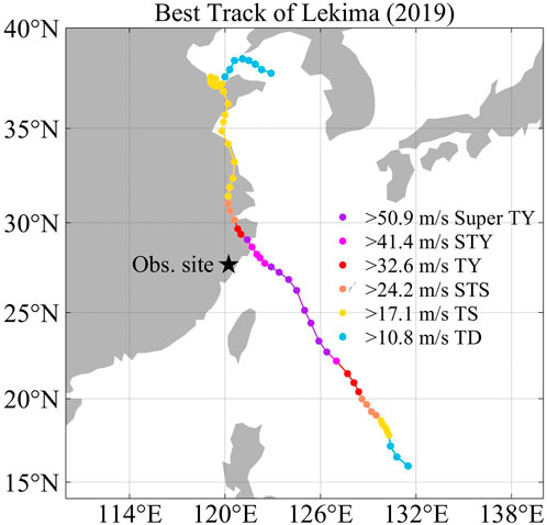
FIGURE 1. Best track of Super typhoon Lekima (2019). Different colors represent different intensities. Super TY: super typhoon, STY: severe typhoon, TY: typhoon, STS: severe tropical storm, TS: tropical storm, and TD: tropical depression. Black star indicates the location of the field experiment.

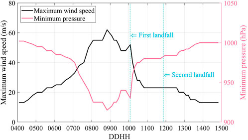
FIGURE 2. Time evolution of the intensity and central pressure of Lekima. Horizontal axis is time in the format of day and hour in August. Vertical axis on the left represents maximum wind speed (unit: m/s), and vertical axis on the right represents minimum pressure (unit: hPa).

Field experiments

To further investigate and understand wind characteristics of typhoon boundary layer, field experiments were performed at East China Typhoon Field Science Experiment Base (Figure 3), which is located in Sansha of Fujian Province as indicated by the black star in Figure 1 (STI, 2022). The closest distance between the observational site and the typhoon center is 181 km based on the best-track data, which is much larger than the radius of maximum wind obtained from Joint Typhoon Warning Center (JTWC, 2022). Therefore, characteristics of wind field outside of the typhoon eyewall are represented by the observations.

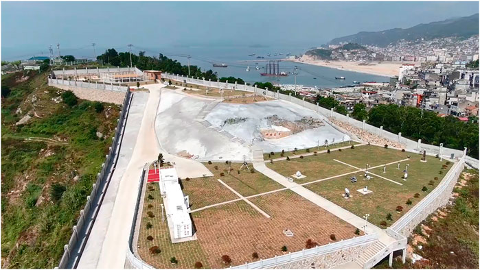
FIGURE 3. East China Typhoon Field Science Experiment Base located in Sansha of Fujian Province as indicated by the black star in Figure 1.

The field experiments include wind tower test equipped with ultrasonic anemometers and DWL test, and their relative positions are shown in Figure 4. The wind tower observation site is located in the north of the DWL observation site, and the distance between these two is 620 m. As shown in Figure 5A, the wind tower is located on a vegetated hillside at an altitude of 44 m. The south and east sides of the tower are close to the sea, and it is 170 m and 100 m away from the coastline on the south and east sides, respectively. The tower is surrounded by hills to the north and west. The tower is equipped with ultrasonic anemometers at four different heights, i.e., 10 m, 30 m, 50 m, and 70 m. The ultrasonic anemometer is WindMaster PRO manufactured by British Gill Company (Figure 6A), which is a precision anemometer offering three-axis wind measurement data and widely used in boundary layer turbulence observation and wind engineering measurements. Operating temperature of this instrument is −40°C to +70°C, the requirement of humidity is <5% to 100%RH, and the allowed precipitation is up to 300 mm/h. The instrument monitors wind speeds of 0–65 m/s with the resolution of 0.01 m/s. It also provides wind direction measurements of 0–360° with the resolution of 0.1°, as well as sonic temperature of −40°C to +70°C with the resolution of 0.01°C. The observation test was conducted from 00:00 on August 9 to 00:00 on August 11, with data output rate of 20 Hz.

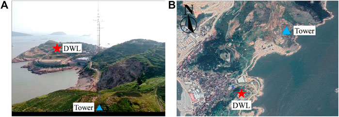
FIGURE 4. Relative positions of wind tower and DWL: (A) Photo of observation sites; (B) Top view of observation sites from map.

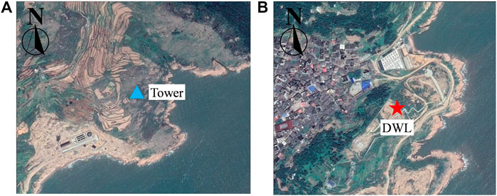
FIGURE 5. Terrain conditions at observation sites: (A) Wind tower; (B) DWL.

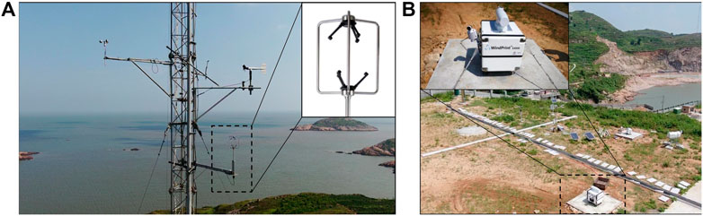
FIGURE 6. Measurement instruments: (A) Ultrasonic anemometer deployed on the wind tower; (B) WindPrint S4000 3D scanning DWL.

Figure 5B shows that the DWL is deployed on a relatively flat site, and the surface is covered with sparse and low grass and shrubs. The altitude of the DWL is 33 m. Its northern and southern sides are close to the sea, and the closest distance to the coastline is 50 m. The deployed DWL is a WindPrint S4000 3D scanning lidar (Figure 6B), which is manufactured by Qingdao Huahang Environmental Technology Co., Ltd. Its scanning cone angle is 60° in DBS (Doppler beam swing) five-beam mode, and its maximum detection distance can reach 4 km. The measurement range of wind speed is 0–75 m/s with the resolution of 0.1 m/s, and the measurement range of wind direction is 0–360° with the resolution of less than 3°. The observation period of the DWL is the same as that of the wind tower, but it has lower internal sampling rate (data output interval: 4 s).

Experimental results and discussion

Before analyzing the experimental results, abnormal data are removed by checking spikes, dropouts, and absolute limits (Hojstrup, 1993; Vickers and Mahrt, 1997; Tang et al., 2022). Signal-to-noise ratio is also checked for DWL data (Tang et al., 2020; Tang et al., 2022). Both wind tower and DWL data are divided into 10-min datasets for data analysis. Therefore, each dataset of wind tower contains 12,000 data points and 150 for DWL data.

Mean wind speed and direction

Figure 7 presents time evolution of 10-min mean wind speed and direction obtained from wind tower measurements and those from DWL measurements. The tower data include four layers of readings from 10 m to 70 m. The maximum measurement height of the DWL can reach 4 km, which is more than enough to cover the height of interest (77.9 m–402.7 m). From Figure 7A, the mean wind speed generally increases as the height increases, and the wind speed gradient is relatively larger before landing than that after landing. Wind speed weakens at the time of landing, and then increases again, reaching a peak at around 06:00 CST on the 10th. The peak wind speed is due to the speed-up effects of the local mountainous terrain. Specifically, after 05:00 CST on the 10th, the center of Lekima passes through a northeast-southwest ridge with an altitude of up to 1.0 km, resulting in compressed wind on the windward side of the hill and hence increased wind speed. After reaching peak speed at 06:00 CST, the mean wind speed gradually decreases. From Figure 7B, the wind blows from the north to the south before landing, and changes to west wind at around 18:00 CST on the 9th. Then, the wind becomes southwesterly and southerly at the time of landing, which is kept unchanged even after the landing. Along the vertical direction, wind directions at 30–70 m are close to each other, while the wind direction at 10 m shifts 20° counterclockwise. Compared to the wind direction at 10 m, wind directions above 70 m shift a little counterclockwise before landing and are close to that at 10 m after landing.

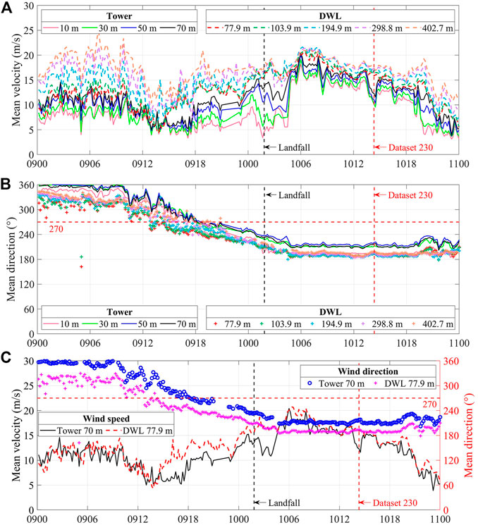
FIGURE 7. Time evolution of 10-min mean: (A) Wind speed (unit: m/s); (B) Wind direction (unit: °); (C) Comparison between wind tower (70 m) and DWL (77.9 m), with vertical axis on the left representing wind speed (unit: m/s) and that on the right representing wind direction (unit: °).

Wind tower data at the height of 70 m and DWL data at 77.9 m are compared in Figure 7C to examine the agreement between these two measurements. Since the tower base is around 10 m higher than that of the DWL, it can be considered that the two observations are performed at the same height. From Figure 7C, general trend and magnitude of wind speeds measured by both instruments are almost the same except for the time period before and after the landing of typhoon, during which wind tower measured wind speed is lower. At that time, prevailing winds start to blow from the west and southwest, and upstream terrain conditions of the wind tower is hilly with an altitude of more than 100 m, while it is residential areas and gentle slopes for the DWL with an altitude of about 40 m. Since hilly terrain with higher altitude exerts stronger shielding effects on the wind field, the associated downstream wind speed is much lower. Therefore, the wind speed measured by the wind tower is lower. Regarding to the wind direction, although the trends of wind tower and DWL data are consistent, the wind direction monitored by the DWL shifts around 30° counterclockwise due to local terrains.

Turbulence intensity

Besides the mean wind, unsteady random motions are also encountered in air flow of typhoon boundary layer, which is referred to as turbulence. Turbulence can be visualized as consisting of eddies (irregular swirls of air motion), which are of many different sizes superimposed onto each other (Stull, 1988). Turbulence intensity is commonly used to characterize turbulence level of the air flow. It is defined as the ratio of standard deviation of the turbulent velocity fluctuations to the mean wind velocity.

Figure 8 presents the time evolution of turbulence intensity at different heights. Time histories of three components of wind velocity are provided for wind tower data, and three-axis turbulence intensities are thus calculated. For DWL data, only horizontal total wind speed is provided, and therefore the total horizontal turbulence intensity is calculated. Although components of wind speed can be back calculated by total wind speed and wind direction, the time resolution of data is found to be degraded. Therefore, original data is used for the calculation of turbulence intensity to guarantee its time resolution. From Figures 8A–C, turbulence intensity generally decreases with the increase of height. At the time of landfall, turbulence intensity tends to increase due to wind speed reduction, which is more obvious at the heights of 10 m and 70 m. After the landfall, the development of turbulence intensity is relatively stable. Figures 8A,B indicate that the magnitudes of turbulence intensity in the along-wind direction and across-wind direction are equivalent before landfall, and the along-wind turbulence intensity becomes higher after landfall; both are higher than the vertical turbulence intensity.

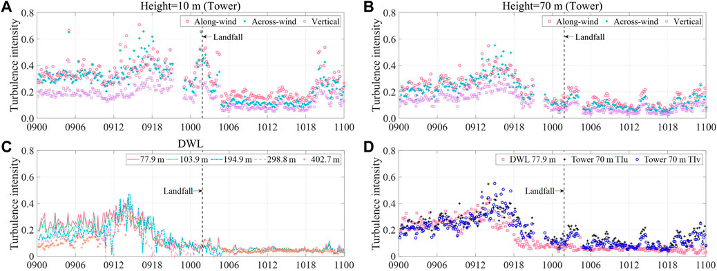
FIGURE 8. Time evolution of turbulence intensity: (A) Tower data at the height of 10 m; (B) Tower data at the height of 70 m; (C) DWL data at five heights (77.9 m, 103.9 m, 194.9 m, 298.8 m, and 402.7 m); (D) Comparison between wind tower (70 m) and DWL (77.9 m).

Figure 8D shows the comparison of turbulence intensity between wind tower data at the height of 70 m and DWL data at 77.9 m. From 00:00 to 15:00 CST on August 9, turbulence intensities measured by both instruments are comparable. Then, turbulence intensity begins to decrease and DWL measured data are lower than wind tower data. This phenomenon is consistent with the time evolution of wind speed as illustrated in Figure 7C, because lower wind speed is mainly associated with higher turbulence intensity due to their inversely proportional relationship. On the other hand, the 100-m-high hill may cause boundary layer separation and vortex shedding on its leeward side, leading to increased wind fluctuations in its wake region where the wind tower is located and therefore higher turbulence intensity is observed.

Profiles of wind speed and turbulence intensity

Since the maximum measurement height of the wind tower is limited to 70 m, DWL data are used to investigate profiles of wind speed and turbulence intensity below the height of 300 m. The power law as given in Eq. 1 is employed to fit the wind speed and turbulence intensity profiles.

where $u\left(z\right)$ and $I\left(z\right)$ are the wind speed and turbulence intensity at the elevation $z$; $z$ is the elevation above the ground; $u_{10}$ and $I_{10}$ are the wind speed and turbulence intensity at the height of 10 m; and $\alpha$ is the power exponent of wind speed profile, and the same $\alpha$ is applied for turbulence intensity profile (GB50009, 2012).

Because $u_{10}$ and $I_{10}$ are not available from DWL measurements, they are first back calculated from recorded data. Then, Eq. 1a is applied to fit the wind speed profile and the power exponent $\alpha$ is determined. A total of five time instants are selected for the investigation of wind speed profiles, which are illustrated in Figures 9A,B. The final fitted power-law profiles are presented in Figures 9C,D.

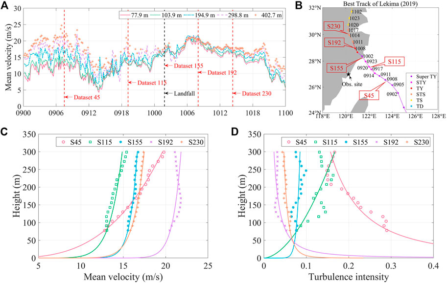
FIGURE 9. Wind speed profile determined based on DWL data: (A) Indication of selected time instants for wind speed profile extraction, with horizontal axis representing time in the format of day and hour and vertical axis representing mean wind speed (unit: m/s); (B) Indication of selected time instants on Lekima’s best track; (C) Power-law fit for wind speed profile; (D) Power-law fit for turbulence intensity profile.

Dataset S45 represents the 10-min period from 07:20 to 07:30 CST on August 9, during which Lekima is categorized as a super typhoon that has not made landfall. The center of Lekima is 331 km away from the DWL. The gradient of mean wind speed is relatively large, and the speed increases by about 7 m/s within the range between 77.9–298.8 m. The power law is used to match with the observations and fit the wind speed profile, with the power exponent $\alpha$ of 0.317 and the coefficient of determination $R^2$ of 0.99. Dataset S115 belongs to the 10-min period from 19:00 to 19:10 CST on the 9^th, during which Lekima degrades to a severe typhoon and is about to make landfall. The typhoon center is 190 km away from the DWL. The exponent of fitted power law is 0.097, and $R^2$ is 0.81. Although a small local reverse of wind speed profile occurs at the height of 120 m, the power law can basically depict the wind speed profile well. Dataset S155 is associated with the time instant of Lekima landfall as a super typhoon. The DWL is 191 km away from the typhoon center. The power exponent is 0.051 and $R^2$ is 0.93 for the fitted power-law profile. Wind speed gradient is relatively small, and the speed only increases by 1–2 m/s within the range between 77.9–298.8 m. The fitted power law agrees with DWL data fairly well. Dataset S192 is from the time instant at 08:00 CST on the 10th after Lekima landfall, with the intensity of typhoon. The DWL is 227 km away from the typhoon center. The $R^2$ of the fitted power law is -0.45 due to the presence of a low-level jet. Peak velocity is reached at the height of 160 m. The power law is not able to match with the DWL data. Dataset S230 indicates the 10-min period from 14:10 to 14:20 on the 10th, which is after Lekima landfall when it is degraded to severe tropical storm. The DWL is 335 km away from the typhoon center. The $R^2$ of the fitted power-law profile of mean wind speed is 0.96, and the power exponent is 0.072, implying that the power law can well describe the mean wind speed profile.

Eq. 1b is applied to fit the profile of turbulence intensity, and the comparison between fitted curve and observations is given in Figure 9D. Datasets S45, S192, and S230 follow the trend that turbulence intensity decreases with height. However, turbulence intensities of datasets S115 and S155 increase as the height increases. Typically, one or more local reverses are observed for turbulence intensity profiles. Turbulence intensities of datasets S115 and S155 experience much larger fluctuations than the remaining, when the typhoon approaches and passes. Also, their $R^2$ for power-law fit are the lowest (smaller than 0.3). Therefore, the power law is incapable of characterizing the shape of turbulence intensity profiles.

CFD simulations and discussion

On top of observational analysis, CFD approach is deployed to simulate the boundary layer of Lekima at Sansha observatory. This section first introduces the setup of CFD simulation of the wind field related to Lekima, then numerical results are validated against wind tower data, and analysis of wind characteristics below 300 m is finally given.

Setup of CFD simulations

Simulated time period and numerical model

Although Lekima lasted for several days, only a certain time period is numerically simulated, which is selected based on two aspects. First, it is assumed that only horizontal wind speed is applied as the velocity input of the CFD simulation for simplification. Therefore, the computational domain is determined according to the wind direction, in order to make flow direction of the domain follow the horizontal wind direction. Figure 10A presents time evolution of mean wind direction below 400 m. Because the wind tower is located at the north of the DWL, the wind direction is required to be in the range between 190° and 270°, so that the wind tower is positioned downstream of the DWL in the computational domain, which can then be served as the benchmark for the validation of CFD simulation. The optimum wind direction is 215° where the wind tower is directly in the downstream of the DWL. Second, the maximum height associated with the data quality ratio exceeding 90% is required to be greater than 400 m to ensure reasonable and reliable observations for the establishment of velocity input. Based on the above considerations, the dataset 230, representing the 10-min period from 14:10 to 14:20 CST on August 10, is selected for CFD simulation. In this dataset, the mean wind direction below 400 m is 195.7°, and the maximum height corresponding to data quality ratio exceeding 90% is 883.3 m.

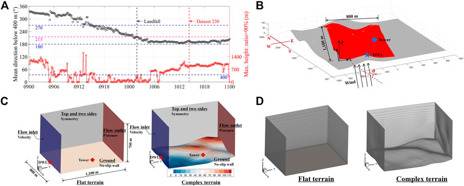
FIGURE 10. Setup of CFD simulation: (A) Time evolution of mean wind direction below 400 m (vertical axis on the left) and the maximum height associated with data quality ratio exceeding 90% (vertical axis on the right); (B) Schematic diagram of computational domain, and the grey color represents the larger region of 2 km × 2 km territory with grids along latitude and longitude, and the red color represents the determined computational domain; (C) Schematic diagram of numerical models with boundary conditions for both flat and complex terrains; (D) Schematic diagram of numerical grids for the two models.

According to the wind direction of 195.7°, the determined computational domain is presented in red in Figure 10B. Flow direction of the computational domain (positive direction of Y-axis) is along the wind direction. The width and length of the computation domain are 800 m and 1,100 m, respectively. To determine the computational domain, a much larger region of 2 km × 2 km is first introduced with grids along latitude and longitude, which is illustrated in grey of Figure 10B. Digital elevation data are derived from NASADEM (2020). Then, the computational domain is determined based on coordinate transformation according to the wind direction of 195.7°, which is the angle $\theta$ in Figure 10B.

On top of the computational domain, the final CFD simulation model is established as shown in Figure 10C, with the height of 700 m in Z direction. The numerical model with a flat terrain is used to validate the boundary conditions at flow inlet, and that with a complex terrain is used to simulate the wind field of typhoon boundary layer. For both numerical models, the same boundary conditions are applied. Velocity inlet and pressure outlet boundary conditions are applied at flow inlet and outlet. The input at the velocity inlet is determined according to DWL measurements. Symmetry-type wall boundary conditions are applied to the top and two sides of the numerical model where a zero flux of all quantities is assumed. No-slip wall boundary condition is applied to the ground where the fluid sticks to the wall. For turbulence modelling with complex terrain, LES as a scale-resolving simulation model is applied. LES directly resolves large scales of motion, and the smaller scales are ignored by filtering the Navier-Stokes equations. The governing equations for LES is given in Eq. 2.

where $\rho$ is the density of air; $t$ is time; $\nu$ is the kinematic viscosity; ${\overline{u}}_i$ and ${\overline{u}}_j$ are filtered velocities, $i$ =1, 2, and 3, and $j$ =1, 2, and 3; $x_i$ and $x_j$ are the Cartesian coordinates in three dimensions; $\overline{p}$ is filtered pressure. ${\overline{\tau }}_{ij}$ is referred to as the subgrid-scale stresses, which are unknown and require additional modelling. Dynamic Smagorinsky-Lilly model is selected as the subgrid-scale model in current study. To solve the governing equations, the segregated solver, semi-implicit method for pressure linked equation-consistent (SIMPLEC), is selected. Second order discretization is used for pressure, bounded central differencing discretization scheme is used for momentum equations, and bounded second order implicit for transient formulation is used.

Numerical models with both flat and complex terrains are discretized into structured mesh (Figure 10D). The grids near the ground are refined in order to accurately capture large velocity gradient. Grid height of the first layer is 0.02 m. Taking the wind speed at the height of 10 m as the reference wind speed and 10 m as the characteristic length, the Reynolds number is estimated to be in the order of ${10}^6$, and Y+ value is estimated to be 350. The total number of numerical grids for both models is 2.35 million.

Determination of velocity input

As mentioned in Simulated Time Period and Numerical Model Section, the velocity input at flow inlet is determined based on DWL data. The time history of DWL measured wind speed associated with dataset 230 is presented in Figure 11A. Because the sampling rate of the DWL is low (about 4 s), time histories of wind speed and direction only exhibit minor fluctuations. In general, wind speed fluctuates between 14 m/s and 20 m/s, and wind direction varies between 185° and 205° below the height of 400 m. To maintain the equilibrium of wind field from inlet to outlet, the equilibrium inflow boundary condition (EIBC) based on Reynolds-averaged Navier-Stokes (RANS) equations (Yang et al., 2009; Zheng et al., 2012) is applied before the running of LES. RANS is another approach to analyze turbulent flows, in which Navier-Stokes equations are averaged over all scales of motion, and only the mean flow is resolved. EIBC is favorable because it considers the applied turbulent kinetic energy to vary with height, which is conventionally assumed to be a constant along height (Richards and Hoxey, 1993). Eq. 3 shows the equations used in EIBC.

where $u\left(z\right)$ is wind speed profile; $\epsilon \left(z\right)$ is the profile of turbulent dissipation rate; $k\left(z\right)$ is the profile of turbulent kinetic energy; $\omega \left(z\right)$ is the profile of specific dissipation rate, which is also used to represent the dissipation of turbulent kinetic energy and similar to turbulent dissipation rate; $u_{*}$ is fiction velocity; $z_0$ is surface roughness length; $\kappa$ is von Kármán’s constant, taken as 0.4; $C_{\mu }$ is model constant, taken as 0.09; $C_1$ and $C_2$ are constants.

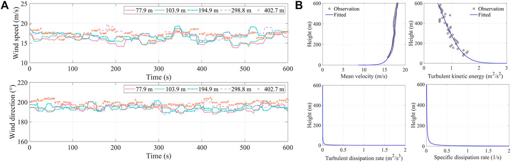
FIGURE 11. (A) Time histories of wind speed (unit: m/s) and wind direction (unit: °) from dataset 230 measured by DWL at five heights, and the horizontal axis is time in seconds; (B) Velocity input at flow inlet in CFD simulations, including mean speed profile (unit: m/s), turbulent kinetic energy profile (unit: m²/s²), turbulent dissipation rate profile (unit: m²/s³), and specific dissipation rate (unit: 1/s).

Equations 3a,c are used to fit profiles of mean wind speed and turbulent kinetic energy from dataset 230 in order to obtain the velocity input. The finalized input for flow inlet is presented in Figure 11B along with observations, and the associated equations are:

Verification of CFD simulations

The EIBC is first validated through numerical simulation associated with the flat terrain (Figure 10C) through RANS. It should be noted that only RANS simulation is conducted for this validation, since it is derived on the basis of RANS. In order to reduce the effects of terrain on the wind field, flat terrain is utilized in the numerical model. As shown in Figure 12A, a total of twenty-one wind speed profiles are extracted from the numerical simulation, and they are very close to each other. In comparison to the velocity input at flow inlet (Eq. 4), the maximum mean error is 0.9 m/s and the maximum root-mean-square error is 0.06 m/s. Therefore, EIBC is effective and valid, and the profile of mean wind speed can be maintained from inlet to outlet.

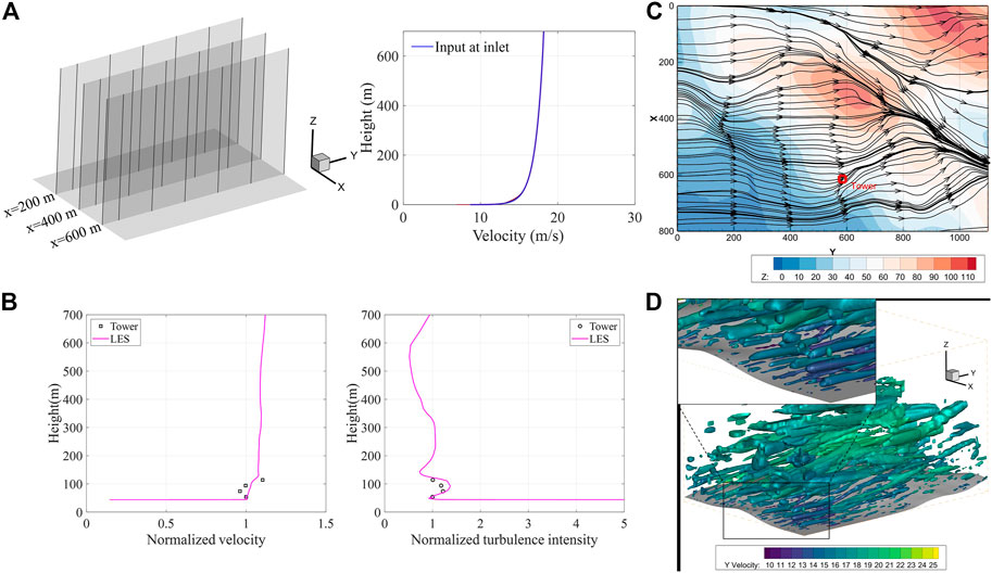
FIGURE 12. Verification of CFD simulations: (A) Equilibrium inflow boundary conditions: (B) Comparison of wind speed and turbulence intensity between numerical results (LES) and wind tower measurements; (C) Mean surface streamline of the wind field and ground elevation (shaded, unit: m), and vertical axis (X) represents across-wind direction in meters, and horizontal axis (Y) represents flow direction in meters; (D) Instantaneous vortex structure of the wind field colored by Y velocity (unit: m/s).

Secondly, LES is validated using the numerical model with complex terrain (Figure 10C), and wind tower data are used as the benchmark. Figure 12B presents the comparison of wind speed profile and turbulence intensity profile between numerical results and wind tower data (dataset 230).

Wind speed profile associated with LES generally increases with height. However, its gradient is smaller than that of observations, and the local reverse occurring in observations is not captured. The reason is that wind direction changes a lot among different heights for wind tower measurements, e.g., wind direction difference between the heights of 10 m and 30 m is up to 20°. Such large variation of wind direction leads to the reverse of wind speed profile at the height of 30 m and large wind speed gradient. However, in the numerical simulation, constant wind direction along height is assumed at flow inlet, ignoring its variation in the vertical direction. Therefore, the simulated wind speed profile differs from the observations regarding the wind speed gradient and the local reverse. The simulated turbulence intensity profile is generally consistent with wind tower data, but with slightly larger magnitude, which corresponds to smaller magnitude of simulated wind speed.

Figure 12C shows the mean surface streamline of the wind field and the ground elevation. According to the shaded ground elevation, there is a small hill with an altitude of 105 m in the middle upper region. West winds prevail on the windward side of the hill and northwesterly winds are formed on the leeward side. At the location where the wind tower stands (red square in Figure 12C), the simulated mean wind direction is about 225°. The mean wind direction determined based on dataset 230 from wind tower data varies in the range of 197°–221°, indicating an error of 1.8%–14.2%.

The simulated instantaneous vortex structure colored by Y velocity is illustrated in Figure 12D. Vortices mainly develop along the flow direction. The scale of vortex near the ground is small due to the influence of terrain and surface friction. Away from the ground, the vortex grows with the height. In summary, the results associated with LES are reasonably consistent with wind tower data and the wind field of typhoon boundary layer can be reproduced by LES. Then, the numerical results are adopted to further understand wind characteristics of typhoon boundary layer below 300 m.

Analysis of wind characteristics

By averaging the instantaneous results from LES, mean wind speed profiles are obtained and presented in Figure 13A in absolute coordinates. Since the apex of the hill in the upper middle region (Figure 12C) is located at X=320 m and Y=620 m, Figure 13A mainly illustrates wind speed profiles on the vertical Y-Z plane where X=320 m to investigate the effects of hilly terrain on wind speed profiles. For uphill winds, six wind speed profiles located at Y=100, 200, 300, 400, 500, and 620 m are extracted. For downhill winds, another six wind speed profiles located at Y=620, 700, 800, 900, 1000, and 1100 m are extracted. For wind speed profiles in the uphill direction, wind speed increases gradually as the ground elevation increases. Along vertical direction, all wind speed profiles obey the law that wind speed increases with height except for the wind speed profile at the apex of the hill (Y=620 m) where a completely reversed and almost monotonically decreasing profile is observed. In the downhill direction, wind speed gradually decreases with the decrease of ground elevation. The reversed wind speed profile is also observed at Y=700 m. Due to local terrain and surface friction, gradient of wind speed is much larger below the height of 300 m while it tends to be stable above 300 m. The same numerical model is also simulated by RANS approach for comparison. Since RANS approach only resolves mean flow, the obtained wind speed profiles are smoother and more consistent with the ideal power law. Because turbulent characteristics of wind field are generated by LES through directly solving large scales of motion, local fluctuations of wind speed profile are observed for LES results, especially below 300 m.

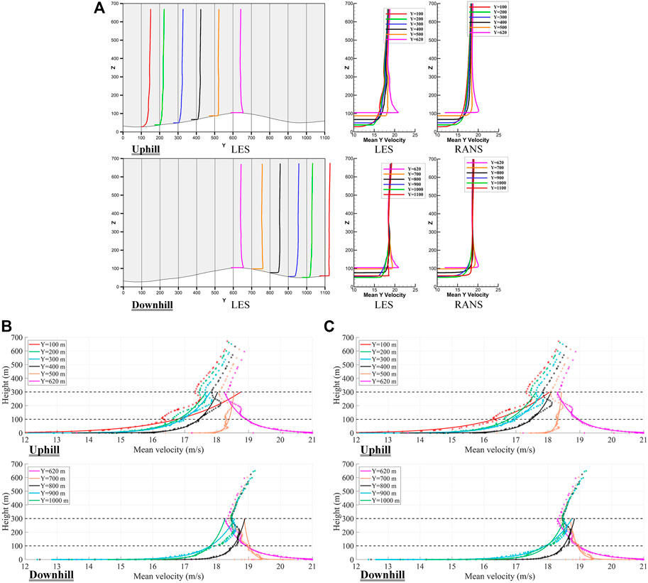
FIGURE 13. Mean wind speed profiles when X=320 m and Y=100–620 m (uphill) or Y=620–1100 m (downhill): (A) Numerical results with absolute coordinates. For subfigures on the left, vertical axis (Z) represents height in meters, and horizontal axis (Y) represents flow direction in meters. For the four subfigures on the right, vertical axis (Z) represents height in meters, and horizontal axis represents mean wind speed; (B) Numerical results (dotted star curves) and fitted power-law profiles (solid curves) between 0 and 100 m with coordinates relative to ground; (C) Numerical results (dotted star curves) and fitted power-law profiles (solid curves) between 0 and 300 m with coordinates relative to ground.

The power law as listed in Eq. 1 is applied to fit the wind speed profiles from LES. Wind speeds below the height of 100 m are first fitted. Comparison between the fitted curve and numerical results is shown in Figure 13B. It should be noted coordinates relative to ground are used for the regression of the power law. From Figure 13B, except for the wind speed profiles at Y=500 m and 700 m, wind speed profiles obtained from LES generally conform to the power-law profile, and fitted curves match the measured data well; the $R^2$ of fitted curves are all greater than 0.96, the maximum mean error is 0.19 m/s and the maximum root-mean-square error is 0.23 m/s. The errors of fitted power-law profile for wind speeds at Y=500 m and 700 m are relatively larger, because both regions are located in the transition zone where the wind speed profile changes from monotonically increasing to monotonically decreasing. Therefore, wind speed profile is more oscillating and fluctuating, which cannot be characterized by the power law that leads to larger deviations. In general, wind speed profiles below the height of 100 m in the uphill and downhill directions obey the law that wind speed increases with height, which can be well depicted by the power law. At the apex of the hill, reverse wind speed profile is observed and the power law with negative exponent can be applied. For the transition zone close to the apex of the hill, the power law can only characterize the development trend of the wind speed profile, neglecting local fluctuations.

The power-law fit for wind speed profiles above 100 m is presented in Figure 13C. Here, wind speeds between 0 and 300 m are used for the power-law fit. From Figure 13C, wind speed profiles no longer follow the monotonically increasing or decreasing law. Local reverses occur at the heights between 110 and 130 m and low-level jets occur at 180–250 m in the uphill direction and at the apex. In the downhill direction, low-level jet normally occurs at the height of 220 m. If the absolute coordinates are applied (Figure 13A), the height where reverse and low-level jet occur is more consistent. Generally, reverse occurs at the height of 125 m, and low-level jet occurs at the height of 290 m in the uphill direction and at the apex. The low-level jet occurs at the height of 270 m in the downhill direction. Due to the above-mentioned inversion and jet, the power law cannot describe mean wind speed profiles above 100 m well. Comparing to parameters from power-law fit based on wind speed data below 100 m, the $R^2$ decreases by 0.11, the mean error increases by 0.08 m/s, and the root-mean-square error increases by 0.07 m/s.

Power exponents of the fitted wind speed profiles between 0–100 m and 0–300 m are correlated to the ground elevation, and linear relation is found, which are calibrated and presented in Eq. 5 and Figure 14.

where $z_g$ is the ground elevation (m); ${\alpha }_{100\mathrm{m}}$ is the power exponent of the fitted wind speed profile below the height of 100 m; and ${\alpha }_{300\mathrm{m}}$ is the power exponent of the fitted wind speed profile below the height of 300 m.

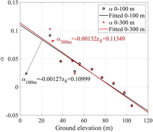
FIGURE 14. Linear relation between power exponents (vertical axis) and ground elevation (horizontal axis). Black solid line represents the fitted relation curve for power exponents obtained from power-law profiles between 0 and 100 m, and black circle represents associated power exponents. Red solid line represents the fitted relation curve for power exponents obtained from power-law profiles between 0 and 300 m, and red plus sign represents associated power exponents.

From Figure 14, power exponents decrease with the increase of ground elevation and even become negative, which corresponds to completely reversed or partially reversed wind speed profiles. Power exponents ${\alpha }_{100\mathrm{m}}$ and ${\alpha }_{300\mathrm{m}}$ slightly differ from each other. Specifically, ${\alpha }_{300\mathrm{m}}$ is larger than ${\alpha }_{100\mathrm{m}}$ when the ground elevation is lower than 80 m. ${\alpha }_{300\mathrm{m}}$ is smaller than ${\alpha }_{100\mathrm{m}}$ when the ground elevation is greater than 80 m.

Figure 15 presents simulated profiles of turbulence intensity. Large variations are observed below the height of 300 m, while the profiles remain almost unchanged above 300 m. For all profiles of turbulence intensity, two local reverses are exhibited, while one is more obvious than the other. In the uphill direction, the dominant local reverse normally occurs at around 120 m and it occurs at around 160 m for the downhill case. Besides, local reverse of turbulence intensity profile typically becomes more significant when ground elevation decreases.

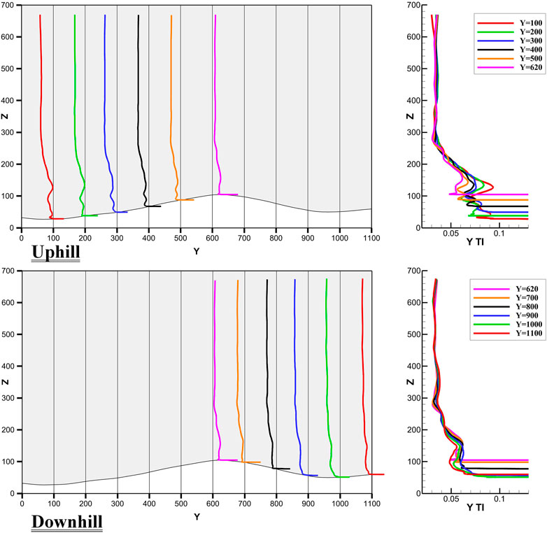
FIGURE 15. Simulated turbulence intensity profiles when X=320 m and Y=100–620 m (uphill) or Y=620–1100 m (downhill). For subfigures on the left, vertical axis (Z) represents height in meters, and horizontal axis (Y) represents flow direction in meters. For subfigures on the right, vertical axis (Z) represents height in meters, and horizontal axis represents turbulence intensity.

Conclusion

This study investigates wind characteristics of atmospheric boundary layer during super typhoon Lekima (2019) by the combination of observational analysis (wind tower equipped with ultrasonic anemometers and DWL) and CFD simulations. The research focuses on the exploration of mean wind speed and turbulence intensity profiles within 300 m (special attention is paid to the height between 100 and 300 m) under the condition of complex terrain. Main conclusions are summarized as follows:

Measurements by wind tower and DWL are compared, and both data are generally consistent with each other. However, due to change of wind direction caused by the approaching of typhoon, upstream conditions of both instruments gradually differ from each other. The measured wind characteristics start to deviate. Therefore, it is necessary to consider wind direction and upstream terrain conditions when analyzing wind characteristics of typhoon boundary layer.

DWL measurements show that mean wind speed profile in the range of 100–300 m cannot be fully described by the power law at different typhoon stages. When typhoon center is far away from the DWL (around 330 km), the power law can well describe the wind speed profile with $R^2$ greater than 0.96. When typhoon is close to the DWL, local reverse and low-level jet are observed for wind speed profile, which cannot be characterized by the power law. Turbulence intensity does not completely decrease with height. When the wind field of typhoon passes the DWL, turbulence intensity increases with height and experiences larger fluctuations.

Based on CFD simulations, mean wind speed below 100 m is fitted for uphill, downhill, hill apex, and transition zone. Power law is able to describe uphill and downhill cases with positive exponent and apex case with negative exponent, while it is less effective for transition zone with local fluctuations. When the height is increased to 100–300 m, local reverse or low-level jet are observed. The $R^2$ of power-law fitted curve is thus reduced by 0.11 compared to that of the power-law fit below 100 m. Simulated turbulence intensity profiles experience local reverses, and degree of reverse is decreased with terrain elevation.

Ground elevation and power exponents of fitted wind speed profiles are successfully correlated with linear relation: power exponents decrease with the increase of ground elevation. However, power exponent becomes negative when ground elevation is greater than 90 m, which corresponds to the apex of the hill.

The above findings are useful to better understand wind characteristics of typhoon boundary layer concentrated between 100 and 300 m. In the future, it is suggested to apply wind direction varying with height in the CFD simulation in order to generate more realistic wind field of typhoons. Also, it is suggested to provide suitable analytical profiles to fit wind speed and turbulence intensity profiles, facilitating wind-resistant design of civil structures in typhoon-prone regions and numerical modelling of typhoons.

Data availability statement

The raw data supporting the conclusion of this article will be made available by the authors, without undue reservation.

Author contributions

TL and ST conducted the study and wrote the manuscript. HQ performed the data analysis and manuscript reviewing and editing. JT, JY, and LL conducted the experimental tests and reviewed the manuscript. YL and YY provided critical feedback on the research.

Funding

This work was supported by the National Key R&D Program of China (No. 2018YFB1501104); National Natural Science Foundation of China (Nos. 42005144, U2142206, 52008316, 41805088); China Postdoctoral Science Foundation (No. 2020M681443); Shanghai Post-doctoral Excellence Program (No. 2020518); Basic Research Fund of Shanghai Typhoon Institute (No. 2022JB01); and Fujian Key Laboratory of Severe Weather Open Foundation (2021TFS02).

Conflict of interest

The authors declare that the research was conducted in the absence of any commercial or financial relationships that could be construed as a potential conflict of interest.

The handling editor (LW) declared a past co-authorship with the author (LL).

Publisher’s note

All claims expressed in this article are solely those of the authors and do not necessarily represent those of their affiliated organizations, or those of the publisher, the editors and the reviewers. Any product that may be evaluated in this article, or claim that may be made by its manufacturer, is not guaranteed or endorsed by the publisher.

References

Blocken, B., van der Hout, A., Dekker, J., and Weiler, O. (2015). CFD simulation of wind flow over natural complex terrain: Case study with validation by field measurements for Ria de Ferrol, Galicia, Spain. J. Wind Eng. Ind. Aerodyn. 147, 43–57. doi:10.1016/j.jweia.2015.09.007
Cao, S., Tamura, Y., Kikuchi, N., Saito, M., Nakayama, I., and Matsuzaki, Y. (2009). Wind characteristics of a strong typhoon. J. Wind Eng. Ind. Aerodyn. 97 (1), 11–21. doi:10.1016/j.jweia.2008.10.002
Chen, P., Yu, H., Xu, M., Lei, X., and Zeng, F. (2019). A simplified index to assess the combined impact of tropical cyclone precipitation and wind on China. Front. Earth Sci. 13 (4), 672–681. doi:10.1007/s11707-019-0793-5
Fang, G., Zhao, L., Cao, S., Ge, Y., and Li, K. (2019). Gust characteristics of near-ground typhoon winds. J. Wind Eng. Ind. Aerodyn. 188, 323–337. doi:10.1016/j.jweia.2019.03.008
GB50009 (2012). Lode code for the design of building structures. Beijing: China Architecture Publishing & Media Co., Ltd.
He, J. Y., He, Y. C., Li, Q. S., Chan, P. W., Zhang, L., Yang, H. L., et al. (2020). Observational study of wind characteristics, wind speed and turbulence profiles during Super Typhoon Mangkhut. J. Wind Eng. Ind. Aerodyn. 206, 104362. doi:10.1016/j.jweia.2020.104362
He, J. Y., Chan, P. W., Li, Q. S., Li, L., Zhang, L., and Yang, H. L. (2022). Observations of wind and turbulence structures of Super Typhoons Hato and Mangkhut over land from a 356 m high meteorological tower. Atmos. Res. 265, 105910. doi:10.1016/j.atmosres.2021.105910
Hojstrup, J. (1993). A statistical data screening procedure. Meas. Sci. Technol. 4 (2), 153–157. doi:10.1088/0957-0233/4/2/003
JTWC (Joint Typhoon Warning Center) (2022). Best track archive. Available at: https://www.metoc.navy.mil/jtwc/jtwc.html?best-tracks (Accessed September 1, 2022).
Law, S. S., Bu, J. Q., Zhu, X. Q., and Chan, S. L. (2006). Wind characteristics of Typhoon Dujuan as measured at a 50m guyed mast. Wind Struct. 9 (5), 387–396. doi:10.12989/was.2006.9.5.387
Li, L., Chan, P. W., Hu, F., Zhang, L. J., and Liu, Y. X. (2014). Numerical simulation on the wind field structure of a mountainous area beside South China Sea during the landfall of typhoon Molave. J. Trop. Meteorol. 20 (1), 66–73.
Li, L., Xiao, Y., Zhou, H., Xing, F., and Song, L. (2018). Turbulent wind characteristics in typhoon Hagupit based on field measurements. Int. J. Distrib. Sens. Netw. 14 (10), 155014771880593. doi:10.1177/1550147718805934
Li, T., Yan, G., Yuan, F., and Chen, G. (2019). Dynamic structural responses of long-span dome structures induced by tornadoes. J. Wind Eng. Ind. Aerodyn. 190, 293–308. doi:10.1016/j.jweia.2019.05.010
Li, T., Yan, G., Feng, R., and Mao, X. (2020). Investigation of the flow structure of single-and dual-celled tornadoes and their wind effects on a dome structure. Eng. Struct. 209, 109999. doi:10.1016/j.engstruct.2019.109999
Li, Y., Zhao, S., and Wang, G. (2021). Spatiotemporal variations in meteorological disasters and vulnerability in China during 2001-2020. Front. Earth Sci. 9, 1194. doi:10.3389/feart.2021.789523
Liao, F., Deng, H., Gao, Z., and Chan, P. W. (2017). The research on boundary layer evolution characteristics of Typhoon Usagi based on observations by wind profilers. Acta Oceanol. Sin. 36 (9), 39–44. doi:10.1007/s13131-017-1109-9
Lu, X., Yu, H., Ying, M., Zhao, B., Zhang, S., Lin, L., et al. (2021). Western north pacific tropical cyclone database created by the China meteorological administration. Adv. Atmos. Sci. 38 (4), 690–699. doi:10.1007/s00376-020-0211-7
Luo, Y. P., Fu, J. Y., Li, Q. S., Chan, P. W., and He, Y. C. (2020). Observation of Typhoon Hato based on the 356-m high meteorological gradient tower at Shenzhen. J. Wind Eng. Ind. Aerodyn. 207, 104408. doi:10.1016/j.jweia.2020.104408
Masters, F. J., Tieleman, H. W., and Balderrama, J. A. (2010). Surface wind measurements in three Gulf Coast hurricanes of 2005. J. Wind Eng. Ind. Aerodyn. 98 (10-11), 533–547. doi:10.1016/j.jweia.2010.04.003
Ming, J., Zhang, J. A., Rogers, R. F., Marks, F. D., Wang, Y., and Cai, N. (2014). Multiplatform observations of boundary layer structure in the outer rainbands of landfalling typhoons. J. Geophys. Res. Atmos. 119 (13), 7799–7814. doi:10.1002/2014jd021637
Nakayama, H., Takemi, T., and Nagai, H. (2012). Large-eddy simulation of urban boundary-layer flows by generating turbulent inflows from mesoscale meteorological simulations. Atmos. Sci. Lett. 13, 180–186. doi:10.1002/asl.377
NASADEM (2020). Release of NASADEM data products. Available at: https://lpdaac.usgs.gov/news/release-nasadem-data-products/(Accessed September 1, 2022).
Powell, M. D., Vickery, P. J., and Reinhold, T. A. (2003). Reduced drag coefficient for high wind speeds in tropical cyclones. Nature 422 (6929), 279–283. doi:10.1038/nature01481
Richards, P. J., and Hoxey, R. P. (1993). Appropriate boundary conditions for computational wind engineering models using the k-ϵ turbulence model. J. Wind Eng. Ind. Aerodyn. 46, 145–153. doi:10.1016/0167-6105(93)90124-7
Shi, W., Tang, J., Chen, Y., Chen, N., Liu, Q., and Liu, T. (2021). Study of the boundary layer structure of a landfalling typhoon based on the observation from multiple ground-based Doppler wind lidars. Remote Sens. (Basel). 13, 4810. doi:10.3390/rs13234810
Song, L., Li, Q. S., Chen, W., Qin, P., Huang, H., and He, Y. C. (2012). Wind characteristics of a strong typhoon in marine surface boundary layer. Wind Struct. Int. J. 15 (1), 1–15. doi:10.12989/was.2012.15.1.001
STI (Shanghai Typhoon Institute) (2022). Opening ceremony of east China typhoon field science experiment base of China meteorological administration. (in Chinese). Available at: https://www.sti.org.cn/gongzuodongtai/2071.html (Accessed September 1, 2022).
Stull, R. B. (1988). An introduction to boundary layer meteorology. Berlin: Springer Science & Business Media.
Tang, S., Guo, Y., Wang, X., Tang, J., Li, T., Zhao, B., et al. (2020). Validation of Doppler wind lidar during super typhoon Lekima (2019). Front. Earth Sci. 16, 75–89. doi:10.1007/s11707-020-0838-9
Tang, S., Li, T., Guo, Y., Zhu, R., and Qu, H. (2022). Correction of various environmental influences on Doppler wind lidar based on multiple linear regression model. Renew. Energy 184, 933–947. doi:10.1016/j.renene.2021.12.018
Tsai, Y. S., Miau, J. J., Yu, C. M., and Chang, W. T. (2019). Lidar observations of the typhoon boundary layer within the outer rainbands. Bound. Layer. Meteorol. 171 (2), 237–255. doi:10.1007/s10546-019-00427-6
Vickers, D., and Mahrt, L. (1997). Quality control and flux sampling problems for tower and aircraft data. J. Atmos. Ocean. Technol. 14 (3), 512–526. doi:10.1175/1520-0426(1997)014<0512:qcafsp>2.0.co;2
Wang, Y., Yin, Y., and Song, L. (2022). Risk assessment of typhoon disaster chains in the guangdong-Hong Kong-Macau greater bay area, China. Front. Earth Sci. 10, 839733. doi:10.3389/feart.2022.839733
WMO (World Meteorological Organization) (2022). Tropical cyclones. Available at: https://public.wmo.int/en/our-mandate/focus-areas/natural-hazards-and-disaster-risk-reduction/tropical-cyclones (Accessed September 1, 2022).
Yang, Y., Gu, M., Chen, S., and Jin, X. (2009). New inflow boundary conditions for modelling the neutral equilibrium atmospheric boundary layer in computational wind engineering. J. Wind Eng. Ind. Aerodyn. 97 (2), 88–95. doi:10.1016/j.jweia.2008.12.001
Yang, Y., Dong, L., Li, J., Li, W., Sheng, D., and Zhang, H. (2022). A refined model of a typhoon near-surface wind field based on CFD. Nat. Hazards 114, 389–404. doi:10.1007/s11069-022-05394-9
Ying, M., Zhang, W., Yu, H., Lu, X., Feng, J., Fan, Y., et al. (2014). An overview of the China Meteorological Administration tropical cyclone database. J. Atmos. Ocean. Technol. 31 (2), 287–301. doi:10.1175/jtech-d-12-00119.1
Zhang, Q., Wu, L., and Liu, Q. (2009). Tropical cyclone damages in China 1983–2006. Bull. Am. Meteorol. Soc. 90 (4), 489–496. doi:10.1175/2008bams2631.1
Zhao, Z., Chan, P. W., Wu, N., Zhang, J. A., and Hon, K. K. (2020). Aircraft observations of turbulence characteristics in the tropical cyclone boundary layer. Bound. Layer. Meteorol. 174 (3), 493–511. doi:10.1007/s10546-019-00487-8
Zheng, D. Q., Zhang, A. S., and Gu, M. (2012). Improvement of inflow boundary condition in large eddy simulation of flow around tall building. Eng. Appl. Comput. Fluid Mech. 6 (4), 633–647. doi:10.1080/19942060.2012.11015448
Keywords: Boundary layer, wind characteristics, computational fluid dynamics, field experiment, typhoon, complex terrain
Citation: Li T, Qu H, Tang S, Tang J, Yan J, Lin L, Li Y and Yang Y (2023) Investigation of wind characteristics of typhoon boundary layer through field experiments and CFD simulations. Front. Earth Sci. 10:1058734. doi: 10.3389/feart.2022.1058734
Received: 30 September 2022; Accepted: 31 October 2022;
Published: 17 January 2023.
Edited by:
Liguang Wu, Fudan University, ChinaReviewed by:
Qingyuan Liu, Chinese Academy of Meteorological Sciences, ChinaJia Liang, Nanjing University of Information Science and Technology, China
Copyright © 2023 Li, Qu, Tang, Tang, Yan, Lin, Li and Yang. This is an open-access article distributed under the terms of the Creative Commons Attribution License (CC BY). The use, distribution or reproduction in other forums is permitted, provided the original author(s) and the copyright owner(s) are credited and that the original publication in this journal is cited, in accordance with accepted academic practice. No use, distribution or reproduction is permitted which does not comply with these terms.
*Correspondence: Shengming Tang, tangsm@typhoon.org.cn