Self-adaptive seismic data reconstruction and denoising using dictionary learning based on morphological component analysis

1 Introduction

The data required for seismic exploration are large and complex, and limited by terrain conditions and the economic cost, seismic data are often irregularly sampled, which may be caused by the complex terrain constraints, including buildings, lakes and forbidden areas for land acquisition (Sun et al., 2021). The inadequate excitation of the artificial source may also result in bad traces, thereby leading to irregular, incomplete and alias frequency of seismic data (Zhang et al., 2019). In order to meet the higher requirements for seismic data quality in subsequent processing, the most direct and effective method is to supplement acquisition and encryption of missing seismic traces (Huo et al., 2013; Zhang et al., 2017). However, restricted by economic cost, it is difficult to re-collect data. Therefore, it is necessary to use effective seismic data reconstruction methods to reconstruct the missing seismic traces in the later period. On the other hand, with the development of seismic exploration to more complex areas and deeper layers, the high elevation difference of topographic relief or the lateral change of near-surface velocity lead to shot excitation and poor receiver conditions, and the random noise interference in the collected single shot records is very strong. If these noises cannot be effectively removed, the migration imaging quality and reservoir prediction accuracy will be affected.

There are four main types of seismic data reconstruction methods. One is the filter-based method (Zhang and Tong, 2003), which using interpolation filtering. However, it usually treats the non-uniform grid sampling data as regular data, which leads to large errors. The second is wave field continuation method (Naghizadeh, 2010), which makes full use of underground information. However, the unknown prior information such as underground structure limits the application of this method. Third, the fast rank reduction method (Gao et al., 2013; Ma et al., 2013), which regards interpolation as an image filling problem, has fast calculation speed and simple parameter setting, but it still has limitations in the reconstruction of irregular missing channels under non-uniform grid sampling and its anti-aliasing ability. The fourth method is the Compressed Sensing (CS) method, which can reconstruct regular and irregular missing seismic traces without any prior information such as underground structures, and has high calculation speed and accuracy. Compressed sensing theory is considered a key method for dealing with the problem of data loss, and the three key factors of CS data recovery are data sparsity, random sampling and optimal reconstruction algorithm (Jiang et al., 2019). Since seismic data are not sparse, it is vital to find suitable sparse dictionaries, so that the coefficients of the signal in the dictionary can remain sparse. Indeed, there are many mathematical transformations used for CS, such as Radon transform (Xue et al., 2014; Tang et al., 2020), Fourier transform (Luo et al., 2015; Wen et al., 2018), Wavelet transform (Cui et al., 2003), Curvelet transform (Zhang et al., 2013; Han et al., 2018; Wang et al., 2018), Seislet transform (Liu et al.,. 2013), etc. (Wang et al., 2021). Seismic data are usually composed of different waves and cannot be fully and effectively represented by a single transformation (Wang et al., 2021). Li et al. proposed the application of Morphological Component Analysis (MCA) to seismic data reconstruction, which separates signals mainly by virtue of the difference between components of different signals (Li et al., 2012). MCA was first proposed to image denoising or restoration and achieved good results. At present, it is widely used in signal denoising, reconstruction, separation, repair and fusion and other fields. Zhou et al. quantitatively evaluated the data reconstruction effect of different sparse dictionary combinations under the framework of MCA, and found that the combination of discrete cosine transform (DCT) and curvelet dictionary is provided with the highest reconstruction accuracy (Zhou et al., 2015). Zhang et al. proposed the combination of the Shearlet and DCT dictionary that can represent seismic data more fully and guarantee more accurate reconstruction data (Zhang et al., 2019). In addition to MCA, many more advanced algorithms have been applied to seismic data processing. In 2014, the Variational Mode Decomposition (VMD) algorithm was first proposed and made a significant achievement in the field of signal decomposition. The VMD is an iterative search for the optimal solution of the variational model to determine what we know about the modes and their corresponding center frequencies and bandwidths. Each mode is a finite bandwidth with a central frequency, and the sum of all modes is the source signal (Dragomiretskiy and Zosso, 2014). Subsequently, many experts and scholars have applied the other decomposition methods to seismic data processing. In 2019, Liu et al. proposed an improved EWT (IEWT) to decompose a non-stationary seismic signal into several IMFs and describe its frequency features. Finally, an adaptive spectrum segmentation using detected boundaries based on the SSR is obtained (Liu et al., 2019). They also first identify the major components of the ground roll adopting the multichannel variational mode decomposition (MVMD), which shows significant improvements compared to the conventional single-channel VMD. Next, separating ground roll and reflections on the selected low-frequency IMFs through a curvelet based blockcoordinate relaxation method (Liu et al., 2021). However, the limitations of the mathematical dictionary remain unchanged. Dictionary learning (DL) is a new representative of interdisciplinary research field, which integrates the theoretical ideas of sparse representation, machine learning, image application and compressed sensing, and is mainly used to solve the problem of dictionary design of sparse representation model. Dictionary learning trains the dictionary according to the characteristics of the processed data, and can get the most adequate dictionary (Wang et al., 2021). K-means algorithm, also known as the clustering algorithm, is considered the simplest dictionary learning method, and detects clusters in the sense of least square error by continuously classifying and updating center points. The K-SVD algorithm (SVD: Singluar Value Decomposition) is an extension of the K-means algorithm, which is also carried out by continuously updating the base and classification (Aharon, 2006). Compared with fixed basis functions, dictionary learning is self-adaptive and can achieve better reconstruction and denoising quality, but its application demands huge time cost and hardware requirements. Yu et al. has made important contributions to the development of dictionary learning, and has successively proposed learning by tight frame, Monte Carlo data driven tight frame, fast rank reduction algorithm, etc., which has improved the efficiency and effect of dictionary learning (Yu et al., 2015; Jia et al., 2016; Yu et al., 2016; Yu et al., 2018). In addition to compressed sensing, machine learning has also been well applied to seismic data reconstruction. SegNet network enables first-arrival picking at the same time as seismic data reconstruction, and forges a solid foundation for the development of data reconstruction and first-arrival picking (Yuan et al., 2022). Liu et al. propose propose a wavelet-based residual DL (WRDL) network to reconstruct the incomplete seismic data. It considers not only features in the time domain but also frequency features of seismic data, which obtains good reconstruction results in real data (Liu et al., 2022).

Compressive sensing usually transforms seismic data into sparse domain by some mathematical transformation method, and then designs a filter in the sparse domain for threshold processing, and then performs mathematical inverse transformation, and finally achieves the purpose of effectively removing noise in seismic data. In the case of the denoising method of seismic data, various theoretical methods have been academically proposed to filter out different types of noise. For regular noise, multiple waves can be removed by Radon transform (Shan et al., 2009), side waves by K-L filtering, and surface waves by least square filtering (Vaidyanathan, 1987). The theoretical basis of these methods is the difference between the effective signal and the regular noise in the characteristics such as frequency and propagation direction. Meanwhile, commonly used algorithms for random noise include frequency domain filtering based on Fourier transform, f-x domain prediction denoising (Spitz, 2012), wavelet transform (Jin et al., 2005), etc. Filtering based on Fourier transform can only filter out the random noise of the lowest and the highest frequency band at both ends; the noise will also be enhanced when the effective signal is enhanced in f-x domain prediction denoising (Spitz, 2012); the wavelet transform performs poorly in expressing the edge information of the curve, and is subject to certain limitations in expressing the hyperbolic features. Liu et al. proposed an EWT-based denoising method in 2020 and effectively suppressed noise. Synthetic data and 3D feld data examples also prove the validity and efectiveness of the TFPF-EWT for both attenuating random noise and preserving valid seismic amplitude (Liu et al., 2020). In this case, as with reconstruction, MCA and dictionary learning are also well applied to the field of denoising. Olshausenp et al. proposed the concept of learned dictionary in 1997, and applied overcomplete dictionary to image denoising. As an advanced and effective signal decomposition method, VMD is also well applied to seismic data denoising. Zhang et al. proposed a multi-channel scheme which is referred as the multi-channel variational mode decomposition (MVMD) based on multi-channel singular spectrum analysis (MSSA), to efficiently and effectively separate and attenuate seismic random noises. This method leverage the MSSA for each decomposed IMF to separate and attenuate random noises (Zhang et al., 2021). Lian et al. took the matching pursuit method as a continuation technique of sparse representation method, and obtained good progress (Lian et al., 2015). Subsequently, Chen proposed the basis tracing method to solve the sparse optimization problem (Chen et al.,. 2001), and Olshausen et al. proposed the self-adaptive learning complete dictionary (Olshausen et al., 2000). Tang et al. first applied the learning complete dictionary to the seismic data denoising. After many times of learning and training of the input signal, the dictionary was updated and the sparse representation coefficient was obtained, which achieved better denoising effect than the traditional method. However, the complexity of the seismic data led to long operation time (Tang et al., 2012). Xu proposed to replace MOD algorithm in K-SVD algorithm with StOMP (Stagewise Orthogonal Matching Pursuit) algorithm, which not only overcomes the over-matching phenomenon caused by orthogonal matching pursuit (OMP) algorithm, but also significantly improves the convergence speed (Xu et al., 2016). With the development of learning methods, Artificial Intelligence (AI) has been gradually applied to seismic data denoising. Zhang et al. proposed a full convolution denoising network based on residual learning, which can remove various noises at the same time (Zhang et al., 2017). Mao et al. proposed a full convolution network, which uses convolution layer to encode to extract features, and deconvolution layer to decode to recover clean data. In recent years, DCNNs has also achieved good results in suppressing random noise (Sang, 2021).

Aiming at the limitations of dictionary combination and the inefficiency of dictionary learning, this paper comes up with a new dictionary library (K-SVD+DCT) and realizes the self-adaptive reconstruction and denoising of seismic data under the MCA framework. In addition, we can also simultaneously reconstruct and denoise to process missing noisy data. Tests of real data have proved the effectiveness and applicability of the proposed method.

2 Theory

2.1 Morphological component analysis (MCA)

Morphological Component Analysis (MCA) uses the individual matching of sparse dictionaries to signal features to achieve signal decomposition. A signal $Y$ consists of $K$ morphological components $x_n$:

where, ${\alpha }_k$ is the sparse coefficient; $D_k$ represents the sparse dictionary. Due to the incoherence between the various morphological components, the solution can be solved by Eq. 2:

Feature selection on data using multiple dictionaries:

To facilitate the solution, we convert Eq. 3 as Eq. 4:

Considering the purpose of decomposing the signal, the vector $\left\{{\alpha }_1,...,{\alpha }_k\right\}$ is transformed into $\left\{X_1,...,X_k\right\}$, representing that the signal contains $K$ morphological components, and each component of the signal is obtained by solving Eq. 5:

2.2 The theory of reconstruction based on MCA

MCA believes that a combined dictionary has the sum of the sparse representation capabilities of its combined components. For example, the combined dictionary of Fourier and Wavelet can well describe signals that contain both stationary and localized features. This is more conducive to the full expression of the data and the improvement of the reconstruction quality. The compressed sensing reconstruction process based on MCA is as follows:

A 2D signal $X$ contains $K$ components of different shapes, which is as Eq. 1. The reconstruction of seismic data can be expressed as follows:

where, $X$ stands for ideal complete seismic data; $Y$ represents the collected data with missing traces; $R$ represents the sampling matrix. In the MCA framework, Eq. 1 can be expressed as:

Above is reformulated as an unconstrained optimization problem:

Where, $\lambda$ is the Lagrange multiplier is used to measure the proportion of ℓ1 norm and ℓ2 norm.

The reconstruction algorithm^’s solution, combined with the BCR (Block Coordinate Relaxation, BCR) algorithm, offered the following solution method based on the morphological component. The solution process is:

Input: sample matrix $R$, the dictionary combination $D=\left[D_1,\cdots ,D_k\right]$, missing seismic data $Y$, the total number of iterations $N$; Output: reconstructed seismic data $X^{\prime }$; Initialize: each morphological component $X_i^{\left(0\right)}=0,i=1,\cdots ,K$.

1) for: $n=1:N$;

2) residual $r^{\left(n\right)}=Y-R\cdot \mathit{sum}\left(X_1,\dots ,X_k\right)$;

3) for: $k=1:K$;

4) ${{\alpha }_k}^{\left(n\right)}=D_k\left({X_k}^{\left(n\right)},\dots ,r^{\left(n\right)}\right)$;

5) ${X_k}^{\left(n\right)}={D_k}^{-1}{T}_{\lambda }\left({{\alpha }_k}^{\left(n\right)}\right)$;

6) the threshold model is applied to reduce $\lambda$;

7) $X^{\prime }=\mathit{sum}\left(X_1,\cdots ,X_K\right)$.

Besides the threshold $\lambda$, we have another independent parameter $p$, which can be flexibly chosen to achieve better performance. Based on the Taylor series, it is valuable to point out that the exponential shrinkage can be considered a smooth ℓ₀ constraint. For $\left|x\right|\ge \lambda$, it is a good approximation of the p-thresholding operator and does not suffer the bias when $p\ne 1$. It reduces to Stein thresholding operator for $p=0$ and soft thresholding for $p=1$. In solving the algorithm, it is necessary to adjust the Lagrange multiplier to get the optimal solution. The steps are as follows: First, a larger transform domain coefficient is selected as the threshold value to obtain the sparse approximate solution. Second, the value is continuously reduced to include more transform domain coefficients, and the optimal solution is approximated by continuous iteration. The threshold selection strategy is called a threshold model, which impacts the algorithm^’s speed and accuracy. Standard threshold models include linear models, exponential models, and data-driven models. In this paper, the exponential model is used, which has the form as:

where, ${\lambda }_{\max }$ and ${\lambda }_{\min }$ stand for the chosen maximum and minimum regularization parameters, respectively. $q_{\max }$ and $q_{\min }$ are user-defined percentages. $N$ is the number of iterations.

2.3 The theory of denoising based on MCA

CS uses the structural differences between the useful signal and random noise in the sparse domain to denoising. A noisy seismic record $y$ and its sparse representation can be expressed as:

where, $\epsilon$ represents random noise; $D$ is a sparse dictionary; $\alpha$ is a sparse coefficient; $x$ is the original signal. Equation 11 can be expressed in the form of MCA as:

To obtain sparse $\alpha$, the following optimization problem is solved using the same method as in 2.2:

3 Dictionary selection

The selection of $D$ is the core problem of the MCA Method. Different dictionaries have a significant influence on the effect of sparse representation. We mainly focus on the overall and local characteristics of seismic data. DFT (Direct Fourier Transformer) and DCT (Discrete Cosine Transform) can be used to transform the overall trend of the data. We take x [n] and y [n] in Figure 1 as an example to illustrate the advantages of DCT. We start by considering the sequence y [n]=x [n]+x [2N-1-n] and this just consists of adding a mirrored version of x [n] to itself. When transform is DFT, we work with extension of x [n], when transform is DCT, we work with extension of y [n]. From Figure 1, it can be seen DFT case the extension introduces discontinuities but this does not happen for the DCT, due to the symmetry of y [n]. The elimination of this artificial discontinuity, which contains a lot of high frequencies, which is the reason why the DCT is much more efficient.

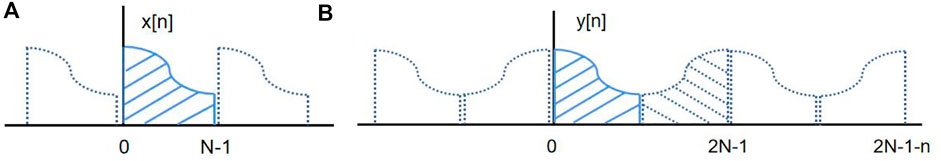
FIGURE 1. Schematic diagram of DFT and DCT. (A)DCT; (B) DCT.

A single mathematical dictionary cannot adequately sparse the representation of seismic data, resulting in loss of information and bad reconstruction data, dictionary learning has been well applied to this problem. Therefor, for the local characteristics of the data, we consider the K-SVD dictionary learning algorithm. We divide the seismic data into two distinct components, so $K=2$. Shearlet transform gets $D_1$ for $k=1$, DCT transform gets $D_2$ for $k=2$. The specific steps for training the dictionary are as follows:

Assuming that there is a training database ${\left\{y_i\right\}}_{i=1}^M$, which can determine the generated model dictionary $A$. Suppose the training error is $\in$, and the goal is to find $A$. Create the following training model:

where, each signal $y_i$ can be expressed as the sparsest representation $A$ on the dictionary $x_i$ to be obtained.

If a dictionary $A$ is obtained whose coefficients are sparse when representing the data, a usable model $R$ can be obtained. Predecessors have proved that when $\in =0$ and all elements in the training database can be represented by $k_0$ ($k_0$ <spark ($A_0$)/2) atoms, there is a unique sparse dictionary $A_0$. Therefore, sparsity can also be used as a constraint, and the goal is to obtain the best fit of the signal, as shown in Eq. 15:

The vectors in the database are combined into a matrix $Y$ by column, and the corresponding sparse representation forms the matrix $X$. The problem of obtaining a dictionary is equivalent to the problem of decomposing matrix $Y$ into $AX$, where the sizes of $A$ and $X$ are fixed and $X$ has sparse columns. The inner layer of Eq. 15 is the sparse problem of representing vector $x_i$ when $A$ is known, and the outer layer is the minimization problem. In the k^th iteration, each element $y_i$ in the database is solved with the dictionary $A_{\left(k-1\right)}$ (the dictionary obtained by the k-1st iteration) to obtain the matrix $X_{\left(k\right)}$, and finally, the Least-Squares is used to solve $A_{\left(k-1\right)}$:

Where, $x_j^T$ represents the j^th row of X. The items in parentheses are used as the known error matrix, which is recorded as Eq. 18:

The optimal $a_{j_0}$ and $x_j^T$ are approximations of $E_{j_0}$ and their rank must be 1. Solving with the SVD algorithm will generate a dense vector $x_j^T$, which increases the number of non-zero items in the $X$ representation. To minimize the known error matrix while keeping all expressed potentials unchanged. We take a subset of the columns in $E_{j_0}$ (the columns in this subset correspond to the signal using the j₀^th atom in the sample set), and the items in the row $x_j^T$ of these columns are non-zero. In this way, only the non-zero coefficient in $x_j^T$ changes, and the potential remains unchanged. The detailed K-SVD dictionary learning algorithm is as follows:

Goal: Obtain the sparse dictionary $A$ by solving the approximate solution of Eq. 15;

Initialize: $k=0$ and:

1) Initialize the dictionary: form $A_{\left(0\right)}\in R^{n\times m}$ (random elements or m randomly selected samples).

2) Normalization: Normalize the columns of $A_{\left(0\right)}$

Main iteration: $k=k+1$, and perform the following steps:

3) Approximate solution using tracking algorithm, get sparse representation $x_i^{\prime }\left(1\le i\le M\right)$, they form the matrix $x_{\left(k\right)}$.

4) K-SVD dictionary update stage: use the following steps to update the columns of the dictionary and obtain $A_{\left(k\right)}$ (repeat $j_0=\mathrm{1,2},\dots ,m$).

1) Define the sample set ${\Omega }_{j_0}=\left\{i|1\le i\le M,X\left(K\right)\left[j_0,j\right]\ne 0\right\}$ that using the atom $a_{j_0}$;

2) Calculate the error ${\mathrm{E}}_{{\mathrm{j}}_0}=\mathrm{Y}-{\displaystyle \sum }_{\mathrm{j}\ne {\mathrm{j}}_0}{\mathrm{a}}_{\mathrm{j}}{\mathrm{x}}_{\mathrm{j}}^{\mathrm{T}}$, where $x_i$ is the j-th row of the matrix $x_{\left(k\right)}$;

3) Limit ${\mathrm{E}}_{{\mathrm{j}}_0}$ by selecting only the column corresponding to ${\mathrm{\Omega }}_{{\mathrm{j}}_0}$ to get ${\mathrm{E}}_{{\mathrm{j}}_0}^{\mathrm{R}}$;

4) Apply SVD to decompose ${\mathrm{E}}_{{\mathrm{j}}_0}^{\mathrm{R}}=\mathrm{U}\Delta {\mathrm{V}}^{\mathrm{T}}$, update the dictionary atom ${\mathrm{a}}_{{\mathrm{j}}_0}={\mathrm{u}}_1$ and the representation ${\mathrm{x}}_{{\mathrm{j}}_0}^{\mathrm{R}}=\Delta \left[\mathrm{1,1}\right]\cdot {\mathrm{V}}_1$.

5) Stop condition: If the change of ${‖\mathrm{Y}-\mathrm{A}{\mathrm{X}}_{\left(\mathrm{k}\right)}‖}_{\mathrm{F}}^2$ is small enough, stop the iteration; otherwise, continue the iteration.

Output: get the result $A_{\left(K\right)}$.

Figures 2,3 show the update process of the K-SVD dictionary. We select a piece of seismic image for the test. We observe that out of a seismic data, less than half were ‘active’ (i.e., non-flat). We randomly choose 100 “active” patches for the dictionary training. The image and examples of ‘active’ patches extracted from it are shown in Figure 2. Figure 3 shows the change of the dictionary after every 5 iterations (from 5th to 40th). As the iterations proceed, the dictionary contains more and more basic features. At the 5^th iteration, the dictionary $A_{\left(5\right)}$ contains only some point features, which are insufficient to express the events. At the 40th iteration, the dictionary $A_{\left(40\right)}$ contains many linear features, and the linear basis functions of various forms are sufficient to achieve the best sparse representation of the seismic data. $E$ is the error of each dictionary and the value is found by Eq. 18. Figure 4 shows the workflow of the method.

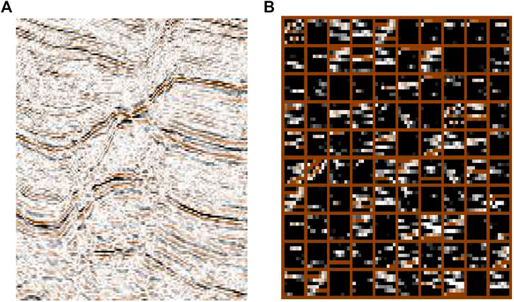
FIGURE 2. Training Set. (A) A seismic image; (B) Examples of non-flat patches.

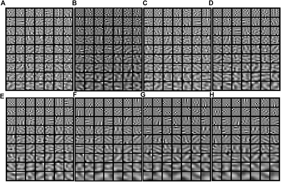
FIGURE 3. Partial dictionary images in different iterations. (A) Partial dictionary images in 5th iterations ($E=17.57$); (B) Partial dictionary images in 10th iterations ($E=15.85$); (C) Partial dictionary image in 15th iterations ($E=14.16$); (D) Partial dictionary images in 20th iterations ($E=10.23$); (E) Partial dictionary images in 25th iterations ($E=6.89$); (F) Partial dictionary images in 30th iterations ($E=3.82$); (G) Partial dictionary images in 35th iterations ($E=1.22$); (H) Partial dictionary images in 40th iterations ($E=0.53$).

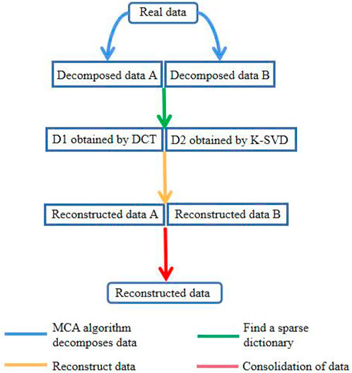
FIGURE 4. Workflow of the proposed method.

4 Test

4.1 Evaluation parameters

To quantitatively describe the reconstruction results, this paper introduces two evaluation parameters, which are defined as follows:

1) Signal Noise Ratio $R_{S/N}$

Where, $X$ represents complete seismic data; $X^{\prime }$ represents a seismic data reconstruction.

2) Peak Signal Noise Ratio $R_{S/N}^P$

Among them, $M_{SE}$ represents mean square error, and its calculation formula is as follows.

4.2 Reconstruction of real data

This paper first verifies the effectiveness of the proposed method for the reconstruction of randomly sampled seismic data by comparing four sets of experimental data. Figure 5A shows a partial image of an offset profile, and Figure 5B depicts the image obtained by randomly sampling 50% of the traces.

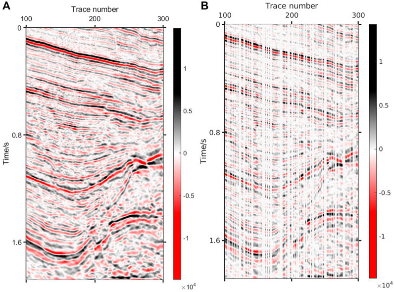
FIGURE 5. Original image and sampled image. (A) Original image; (B) 50% missing data (SNR=3.03 dB PSNR=19.38 dB).

The proposed method can effectively reconstruct the underground medium image in the case of a low sampling rate. It can be seen from Figure 6 that the proposed method can not only reconstruct the shallow reflection images, but the deep weak reflection images are also well reconstructed. Figure 6A presents the reconstruction result of DCT+K-SVD; Figure 6B describes the reconstructed error, which represents reconstructed quality without noise. Figures 6C,D show the reconstruction components of K-SVD and DCT. It can be seen that the reconstruction amount of K-SVD for small structures is rich, and most structures that cannot be accurately reconstructed by fixed dictionaries are well restored by K-SVD. The simple structures, such as smooth events and strong low-frequency signal, can be easily reconstructed by DCT, which greatly reduces the calculation amount of dictionary learning and improves the efficiency. Figure 7 shows the reconstruction results of K-SVD. Due to the optimal expression of dictionary learning algorithm, K-SVD can reconstruct seismic data with very high accuracy. However, it will take a lot of time, which is particularly obvious when processing huge real data. Figure 8 shows the reconstruction result of Curvelet+DCT. Figure 8A reveals that although this method can recover all the missing information, the reconstructed data have insufficient energy, the details are clearly depicted, and the microstructure cannot be distinguished, while Figure 8B suggests the existence of errors at various locations in the reconstructed data. It can be seen from Figures 8C,D that the two dictionaries (Curvelet and DCT) have limited recovery ability for small structures. Curvelet transform is applicable to signals with curve characteristics, but DCT cannot perfectly reconstruct the remaining signals. In contrast, the Shearlet method is provided with a stronger reconstruction ability, which combines multi-scale geometric analysis through synthetic wavelet theory and affine system, and generates the basis function by stretching, translating, and rotating a base function. However, its lack of global sparse representation ability gives rise to reconstruction noise caused by undersampling in the reconstruction data, as shown in Figure 9A. Figure 10 indicates that the DCT method can completely supplement the missing data, but its detail-describing ability is poor, and the image cannot be reconstructed with a high resolution. To further compare the reconstruction effects of the four methods, the 221th trace is taken for a separate comparison, and the results are shown in Figure 11. It can be seen from the curves that the results obtained by the proposed method have the best fit with the original signal. The Shearlet+DCT and Shearlet method is seriously inconsistent in some areas (For example, 0.6 s–0.7 s and 1.4 s–1.5 s). The curve of the signal obtained by the DCT and shearlet method poorly fits the original signal. Table 1 shows the quantitative evaluation parameters of the five methods, of which the proposed method has the highest improvement in SNR and takes less time than K-SVD.

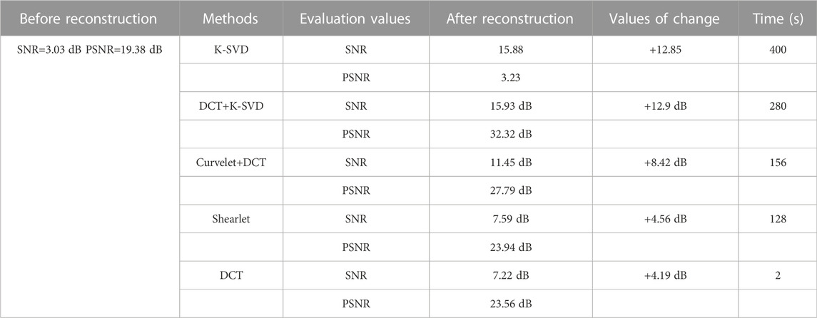
TABLE 1. Evaluation values for different methods.

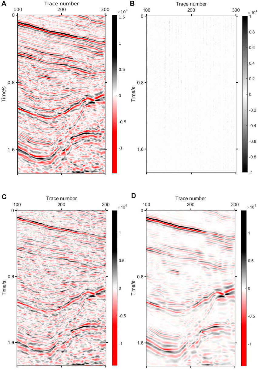
FIGURE 6. Result via DCT+K-SVD. (A) Result via DCT+K-SVD (SNR=12.1 dB PSNR=28.45 dB); (B) Absolute error via DCT+K-SVD; (C) Reconstruction component via K-SVD; (D) Reconstruction component via DCT.

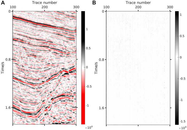
FIGURE 7. Result via K-SVD. (A) Result via K-SVD (SNR=15.88 dB PSNR=33.23 dB); (B) Absolute error via K-SVD.

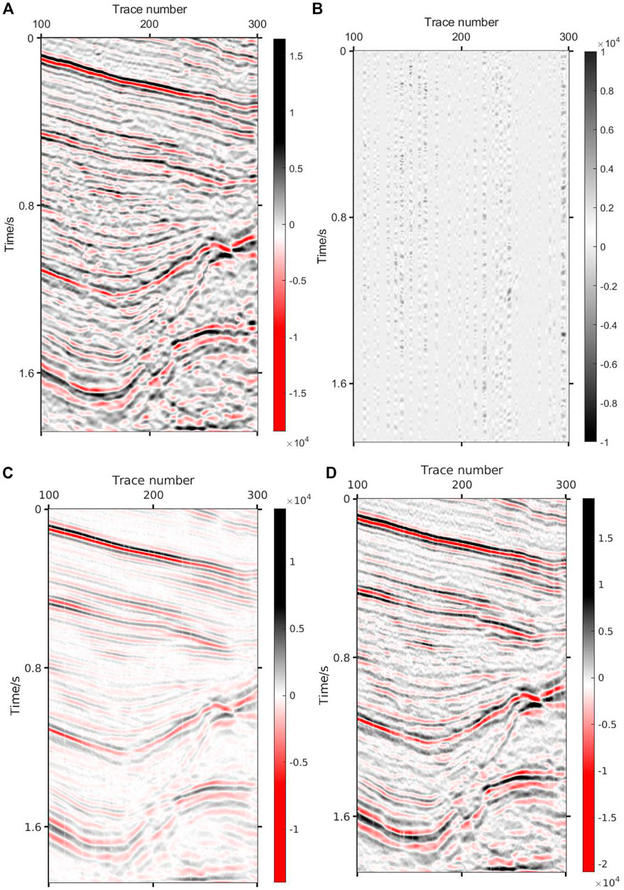
FIGURE 8. Result via Curvelet+DCT. (A) Result via Curvelet+DCT (SNR=11.45 dB PSNR=27.79 dB); (B) Absolute error via Curvelet+DCT; (C) Reconstruction component via Curvelet; (D) Reconstruction component via DCT.

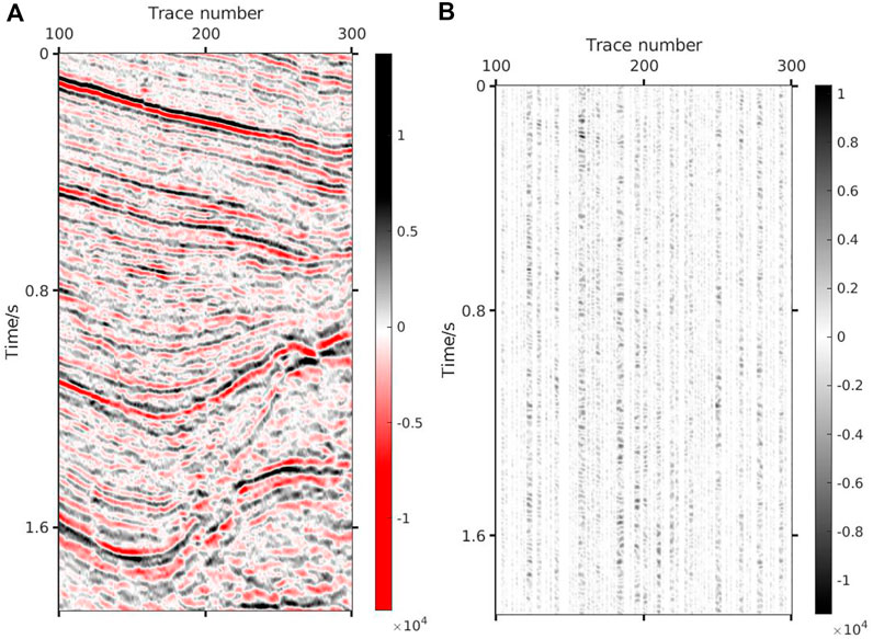
FIGURE 9. Result via Shearlet. (A) Result via Shearlet (SNR=7.59 dB PSNR=23.94 dB). (B) Absolute error via Shearlet.

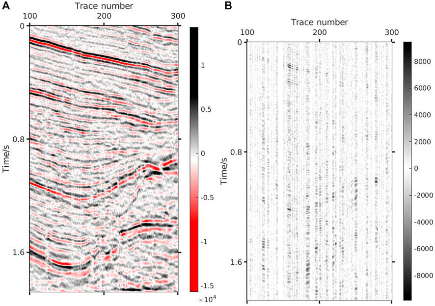
FIGURE 10. Result via DCT. (A) Result via DCT (SNR=3.03 dB PSNR=23.56 dB). (B) Absolute error via DCT.

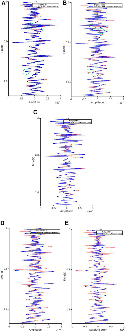
FIGURE 11. Reconstructed single trace result (Red: Original data 221th trace; Blue: Reconstructed data 221th trace). (A) Single trace result via DCT+K-SVD; (B) Single trace result via Curvelet+DCT; (C) Single trace result via K-SVD; (D) Single trace result via Shearlet; (E) Single trace result via DCT.

The following conclusions can thus be drawn from numerical experiments: 1) DCT+K-SVD, Shearlet and DCT reconstruction methods based on CS can complement the missing data at lower sampling rates, while it is difficult for the Curvelet+DCT method to complete the reconstruction. This is because the Curvelet will recognize it as a boundary in the large vacancy position, and the Curvelet is equipped with good boundary protection properties, making it impossible to reconstruct the large missing location; 2) Sparse transformation is the key to the reconstruction algorithm, with sparser coefficients obtained after transformation indicating a better reconstruction effect. This group of experiments shows that Shearlet presents better reconstruction results than DCT because of the multi-directional and multi-scale characteristics of Shearlet transform, representing the signal more sparsely; 3. The hereby proposed reconstruction method based on the DCT+K-SVD sparse transformation can well reconstruct the underground medium. Overall, the difference from original images is the smallest, while that from SNR and PSNR are the biggest. The weak reflection image at the bottom is also endowed with a better reconstruction effect in terms of local details.

In order to explore the reconstruction ability of the proposed method, data are reconstructed with different degrees of random missing, including 20%, 40%, 60%, and 80%. The missing data with four missing levels, the reconstruction results and the errors are presented in Figure 12, where it can be noticed that the reconstruction effect gradually decreases with the increase of the number of deletions. However, it can be guaranteed that the proposed method can maintain satisfactory results in the case of less than 60% missing. When 80% of the data are missing, although some small features cannot be perfectly reconstructed, the information of the reconstructed data is complete, the event axis is continuous, and the SNR is improved. However, it can be seen from Figures 13D,H that other dictionary combination methods (Curvelet+DCT) are difficult to completely reconstruct a large number of missing data, and their reconstructed data have discontinuous events and low SNR ratio. Table 2 shows the parameters of K-SVD+DCT before and after reconstruction of data with different missing degrees.

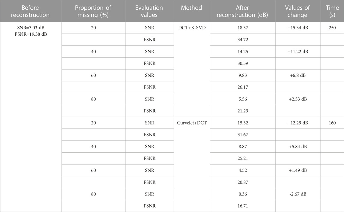
TABLE 2. Evaluation values for different missing.

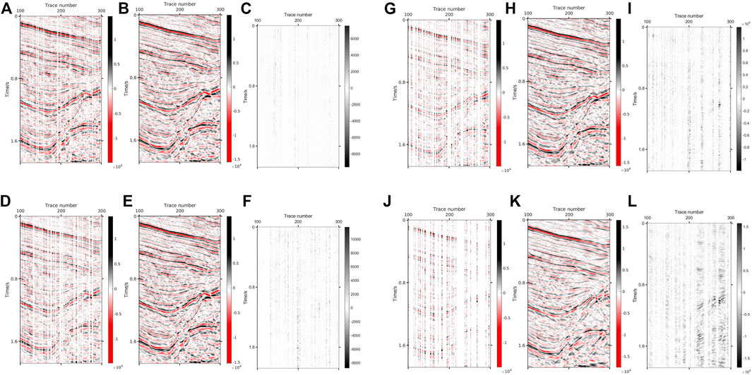
FIGURE 12. DCT+K-SVD results via missing in different proportions. (A) 20% missing image. (B) Reconstructed result via 20% missing (SNR=18.37 dB PSNR=34.72 dB). (C) Absolute error via 20% missing; (D) 40% missing image. (E) Reconstructed result via 40% missing (SNR=14.25 dB PSNR=30.59 dB). (F) Absolute error via 40% missing. (G) 60% missing image. (H) Reconstructed result via 60% missing (SNR=9.83 dB PSNR=26.17 dB). (I) Absolute error via 60% missing; (J) 80% missing image. (K) Reconstructed result via 80% missing (SNR=0.5 dB PSNR=21.29 dB). (L) Absolute error via 80% missing.

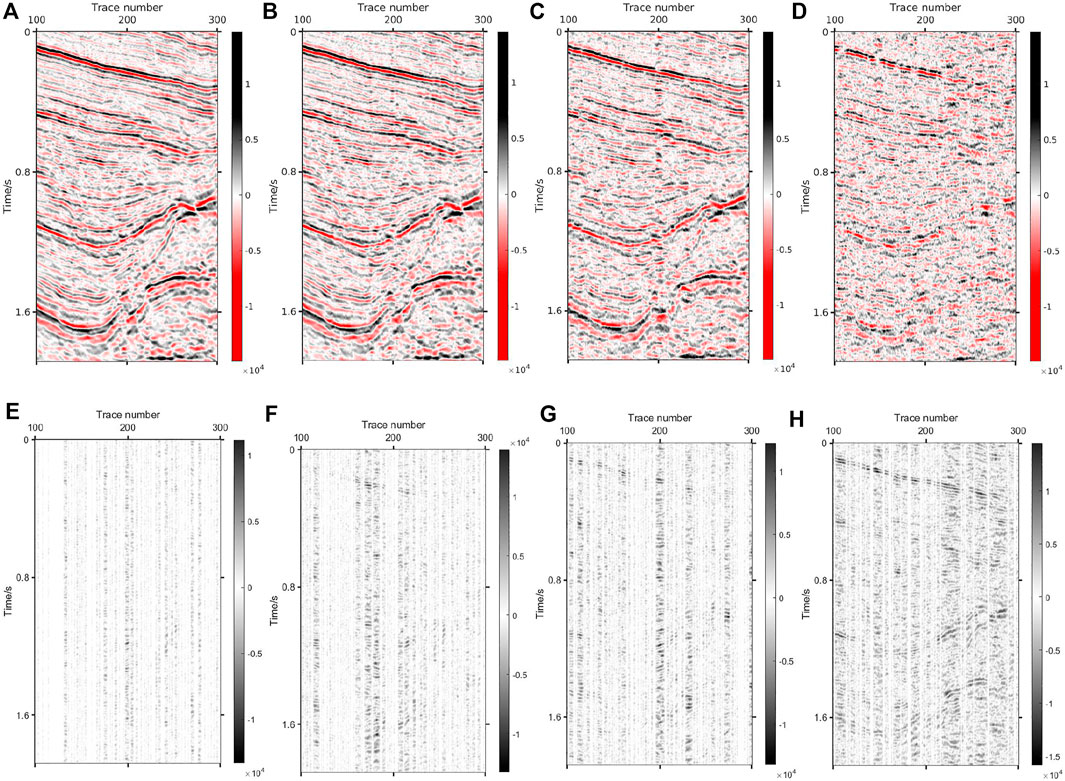
FIGURE 13. Curvelat+DCT results via missing in different proportions. (A) Reconstructed result via 20% missing (SNR=15.32dBdB PSNR=31.67 dB). (B) Reconstructed result via 40% missing (SNR=8.87 dB PSNR=25.21 dB). (C) Reconstructed result via 60% missing (SNR=4.52 dB PSNR=20.87 dB). (D) Reconstructed result via 80% missing (SNR=0.36 dB PSNR=16.71 dB). (E) Absolute error via 20% missing; (F) Absolute error via 40% missing. (G) Absolute error via 60% missing; (H) Absolute error via 80% missing.

The real seismic data of a certain work area are used to test the applicability of the method. The humid climate caused water accumulation in the ground, and multiple receivers on the survey line are damaged, resulting in incomplete acquisition data. Figure 14 is a partial display of the original data. Multiple breaks can be observed in the events, which will be further reconstructed to get complete data and smooth events. Figure 14B shows the reconstruction result, and all the missing data are found to have been recovered. In addition, the events of the reconstructed data are smooth and continuous, and the SNR of the data is also improved.

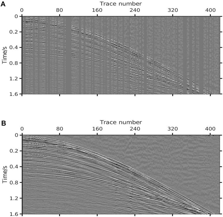
FIGURE 14. Regularized reconstruction of real data. (A) Original data (SNR=2.16 dB PSNR=11.2 dB). (B) Reconstructed data (SNR=23.89 dB PSNR=32.92 dB).

4.3 Denoising of real data

The proposed method is hereby applied to Compressed Sensing denoising that uses the differences between useful signal and random noise in sparse domain for denoising. In order to verify the effectiveness of the method, a part of the offset profile is selected for the experiment. The data have a total of 350 traces and 800 sampling points, as shown in Figure 15. Figure 15B describes the data with noise, the main frequency of which is 40 Hz. DCT+K-SVD is hereby compared with DCT and Shearlet+DCT to prove its superiority. Figures 16–18 are the denoising result and the removed noise of the three methods. Figure 16 depicts the denoising result of the proposed method, and suggests that the method can efficiently extract useful signals of the deep and shallow layers. Additionally, this method does not cause any information loss and better retains the original data characteristics. Figure 17 shows that the denoising ability of the DCT method is weak and fails to effectively suppress random noise. In contrast, the Shearlet method has a stronger denoising ability and can basically suppress all the noise. However, due to the lack of self-adaptation, this method is still subject to the problem that the useful signals are suppressed, and the removed useful signals can be seen from Figure 18. Table 3 shows the noise reduction evaluation parameters of the three methods. The denoising ability of the proposed method is tested under different degrees of random noise, including 20Hz, 35Hz, 50Hz, and 65 Hz. Figure 19 shows the noisy data with four levels, the denoising results and the removed noise, and it can be observed from Figure 19J that even under the interference of strong noise, the effective signal is covered by a large area, making it still possible to extract useful signals and obtain satisfactory denoising results. Table 4 shows the relevant parameters.

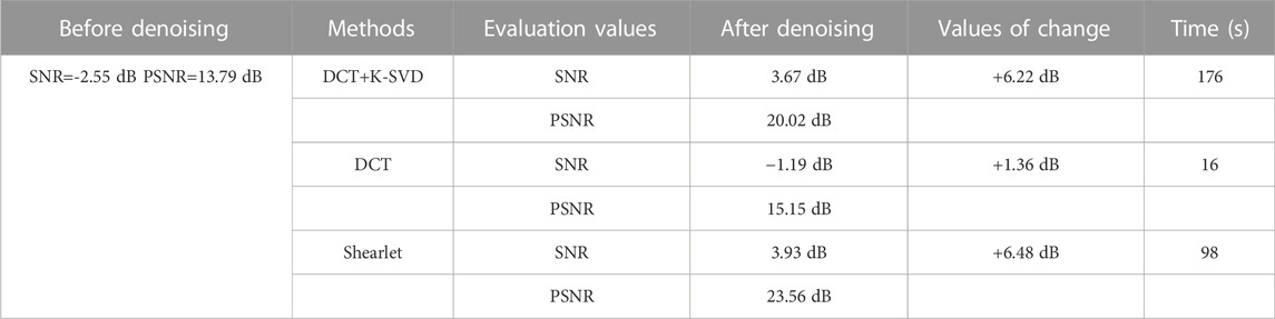
TABLE 3. Evaluation values for different methods.

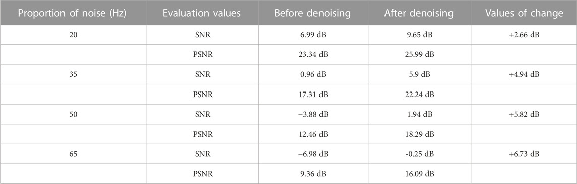
TABLE 4. Evaluation values for different noise.

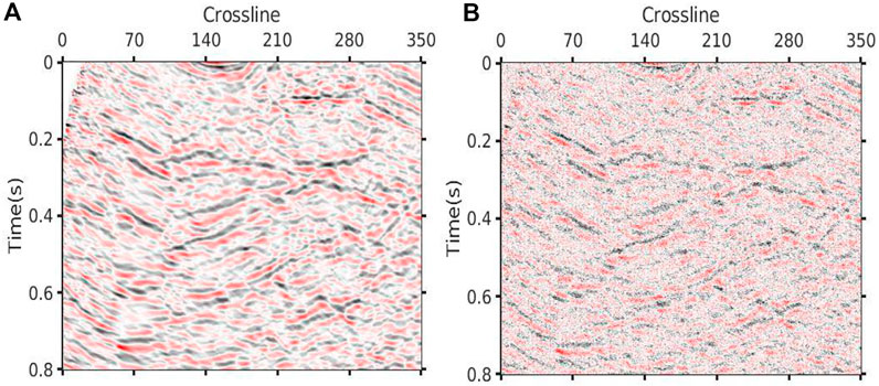
FIGURE 15. Original image and noisy image. (A) Original image. (B) Noisy image (SNR=−2.55 dB PSNR=13.79 dB).

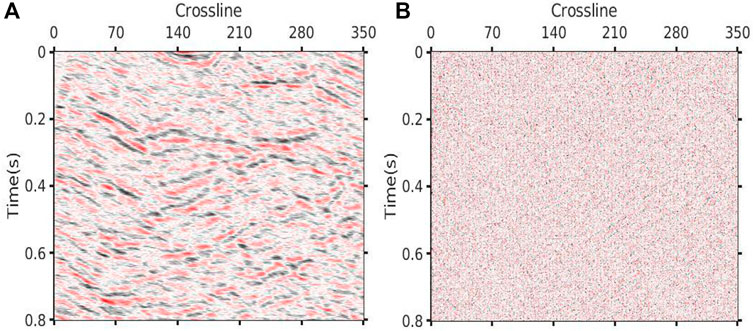
FIGURE 16. Denoising result via DCT+K-SVD. (A) Denoised data (SNR=3.67 dB PSNR=20.02 dB). (B) Removed noise.

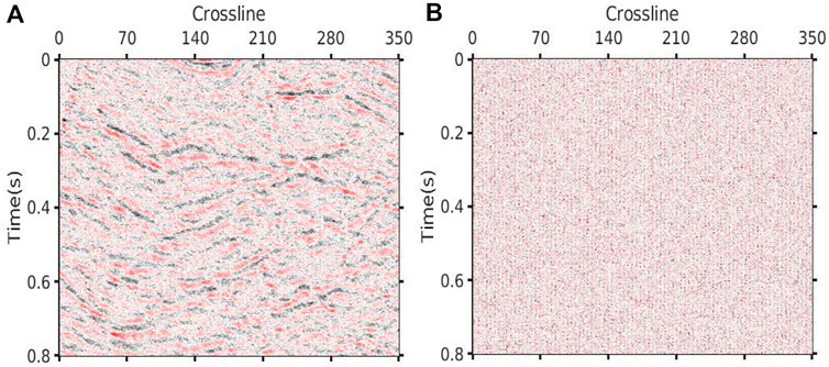
FIGURE 17. Denoising result via DCT. (A) Denoised data (SNR=−1.19 dB PSNR=15.15 dB). (B) Removed noise.

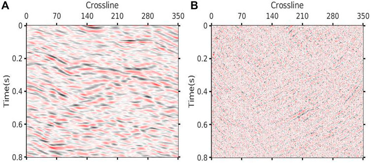
FIGURE 18. Denoising result via Shearlet. (A) Denoised data (SNR=3.93 dB PSNR=20.28 dB). (B) Removed noise.

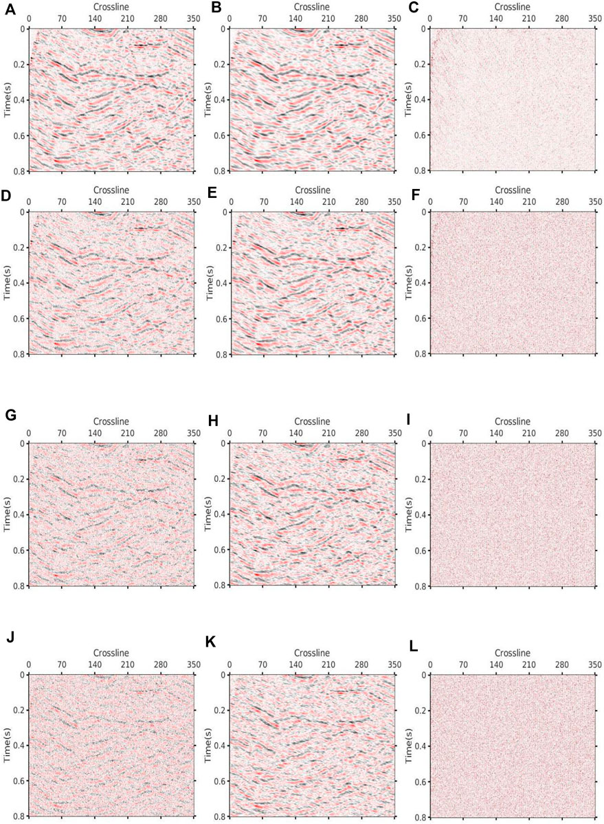
FIGURE 19. DCT+K-SVD denoising results via different levels of noise. (A) Image with 20 Hz noise (SNR=6.99 dB PSNR=23.34 dB). (B) Denoised data via 20 Hz noise (SNR=9.65 dB PSNR=25.99 dB). (C) Removed noise via 20 Hz noise. (D) Image with 35 Hz noise (SNR=0.96 dB PSNR=17.31 dB). (E) Denoised data via 35 Hz noise (SNR=5.9 dB PSNR=22.24 dB). (F) Removed noise via 35 Hz noise. (G) Image with 50 Hz noise (SNR=−3.88 dB PSNR=12.46 dB). (H) Denoised data via 50 Hz noise (SNR=1.94 dB PSNR=18.29 dB). (I)Removed noise via 50 Hz noise. (J) Image with 65 Hz noise (SNR=−6.98 dB PSNR=9.36 dB). (K) Denoised data via 65 Hz noise (SNR=−0.25 dB PSNR=16.09 dB). (L) Removed noise via 65 Hz noise.

To verify the applicability of this denoising method, the real data, a single shot record of a work area in western China, with a total of 800 traces and a sampling time of 2.5s, are further processed. Figure 19A reveals that the data contain a lot of noise. The existence of random noise and linear line noise makes the SNR of the shot set data low, and the continuity of the event is poor. Figure 20B shows the denoising result of DCT+K-SVD, indicating that most of the random noise is effectively suppressed, and that the event between 1.25 m and 1.5 m is clearer. The SNR of the data has been significantly improved, and forged a good foundation for subsequent processing. Figure 19C depicts the removed noise, and reveals that not only random noise is removed, but some linear noise and surface waves are also suppressed to a certain extent. The reason is that the dictionary learning algorithm self-adaptively learns the characteristics of the useful signal that can effectively distinguish the useful signal from other signals.

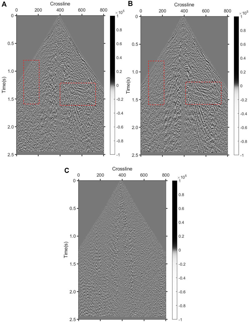
FIGURE 20. Real data denoising. (A) Original data (SNR=1.69 dB PSNR=26.79 dB). (B) Denoised data (SNR=5.93 dB PSNR=31.02 dB). (C) Removed noise.

4.4 Process of real missing noisy data

This section presents the comprehensive application of the proposed method, based on which, the reconstruction and denoising of missing noisy data are implemented. Original data and processed data are shown in Figure 21. Figure 21A describes the original data, where partial missing and random noise can be observed. Figure 21B reveals that all the missing information is accurately recovered, and that the SNR is also significantly improved.

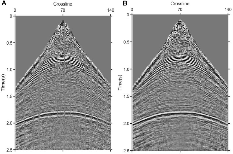
FIGURE 21. Real data processing. (A) Original data (SNR=13.61B PSNR=37.91 dB). (B) Reconstruct the denoised data (SNR=22.19 dB PSNR=46.49 dB).

5 Conclusion

Problems such as missing tracks and bad tracks generally give rise to the incompletion of the seismic data. From the inversion perspective, incomplete image reconstruction is an ill-posed inverse problem, and seismic signals are inevitably affected by noise during the propagation process, which reduces the quality of seismic data and brings difficulties to subsequent interpretation work. However, compressed sensing reconstructs the data using the sparsity of the signal, and is well applied in the fields of regular reconstruction and denoising.

A new dictionary combination, i.e., K-SVD+DCT, is hereby proposed under the MCA framework, which overcomes the limitation of fixed base functions by training dictionaries fully suitable for processed data. DCT is a global type transformation used to reconstruct a smooth event. Therefore, the coefficients of the signal obtained using K-SVD+DCT are sparser, and have a good reconstruction and denoising effect on both pre-stack and post-stack data. Considerable experiments show that the hereby proposed method can reconstruct the image well, that the relative error of the reconstruction result is limited, and that the local details and the deep weak reflection signal can also be well reconstructed. Besides, even under the interference of strong noise, the effective signal is covered by a large area, and it is still possible to extract useful signals and obtain satisfactory denoising results. Indeed, this method retains both the fast operation of mathematical transformations and the high precision of dictionary learning. However, only the training time of dictionary learning is reduced by reducing the training data. To this end, the focus of future work will be placed on improving the dictionary learning time and developing efficient dictionary learning algorithms.

Data availability statement

The raw data supporting the conclusions of this article will be made available by the authors, without undue reservation.

Author contributions

The first author DW is the first owner of the research results, responsible for algorithm research and article writing, XX and HZ are in charge of auxiliary research.

Funding

This study was supported by the Research on Full-Frequency Processing Method of Thin Reservoir and Research on Target Fine Characterization Technology Research (2022KT1503) and Research and realization of seismic pre-stack imaging in the western segment of Kedong structural belt in southwestern Tarim Basin in 2022 (2022KT0506).

Conflict of interest

The authors DW, XRX, HZ, JS and XX were employed by PetroChina. The author YZ was employed by Wuhua Energy Technology Co., Ltd.

Publisher’s note

All claims expressed in this article are solely those of the authors and do not necessarily represent those of their affiliated organizations, or those of the publisher, the editors and the reviewers. Any product that may be evaluated in this article, or claim that may be made by its manufacturer, is not guaranteed or endorsed by the publisher.

References

Aharon, M., Elad, M., and Bruckstein, A. K. S. V. D. (2006). $rm K$-SVD: An algorithm for designing overcomplete dictionaries for sparse representation. IEEE Trans. Signal Process. 54 (11), 4311–4322. doi:10.1109/TSP.2006.881199
Chen, S. S., Donoho, D. L., and Saunders, M. A. (2001). Atomic decomposition by basis pursuit. SIAM Rev. Soc. Ind. Appl. Math. 43 (1), 129–159. doi:10.1137/s003614450037906x
Cuifuqi, X. D., and Zhang, G. (2003). Seismic traces interpolation using wavelet transform[J]. Oil Geophys. Prospect. 38 (S1), 93–97.
Dragomiretskiy, K., and Zosso, D. (2014). Variational mode decomposition. IEEE Trans. Signal Process. 62 (3), 531–544. doi:10.1109/tsp.2013.2288675
Gao, J. J., Sacchi, M. D., and Chen, X. H. (2013). A fast re-duced-rank interpolation method for prestack seismic volumes that dependon four spatial dimensions. Geophysics 78 (1), V21–V30. doi:10.1190/geo2012-0038.1
Hanliang, L. (2018). The study on seismic data reconstruction method based on curvelet transform. : China University of Petroleum (EastChina), Qing-dao, Shandong
Huo, Z., Deng, X., and Zhang, J. (2013). The over view of seismic data reconstruction methods. Prog. Geophys. 28 (4), 1749–1756.
Jia, Y., Yu, S., Liu, L., and Ma, J. (2016). A fast rank-reduction algorithm for three-dimensional seismic data interpolation. J. Appl. Geophys. 132, 137–145. doi:10.1016/j.jappgeo.2016.06.010
Jiang, P., Zhang, K., Zhang, Y. K., and Tian, X. (2019). Noisy seismic data reconstruction method based on morphological component analysis framework. Prog. Geophys. 34 (2), 573–580.
Jin, Y., Angelini, E., and Laine, A. (2005). Wavelets in medical image processing: De-noising, segmentation, and registration[J]. Behav. Process. 45 (1-3), 33–57. doi:10.1007/0-306-48551-6_6
Li, H., Wu, G., and Yin, X. (2012). Morphological component analysis in seismic data reconstruction[J]. Oil Geophys. Prospect. 47 (2), 236–243.
Lian, Q. S., Shi, B. S., and Chen, S. Z. (2015). Research advances on dictionary learning models, algorithms and applications. Acta Autom. Sin. 41 (2), 240–260. (in Chinese).
Liu, N., Li, F., Wang, D., Gao, J., and Xu, Z. (2021). Ground-roll separation and attenuation using curvelet-based multichannel variational mode decomposition. IEEE Trans. Geosci. Remote Sens. 60, 1–14. doi:10.1109/tgrs.2021.3054749
Liu, C., Li, P., Liu, Y., Wang, D., and Liu, D.-M. (2013). Iterative data interpolation beyond aliasing using seislet transform. Chin. J. Geophys. 56 (5), 1619–1627.
Liu, N., Li, Z., Sun, F., Wang, Q., and Gao, J. (2019). The improved empirical wavelet transform and applications to seismic reflection data. IEEE Geosci. Remote Sens. Lett. 16 (12), 1939–1943. doi:10.1109/lgrs.2019.2911092
Liu, N., Wu, L., Wang, J., Wu, H., Gao, J., and Wang, D. (2022). Seismic data reconstruction via wavelet-based residual deep learning. IEEE Trans. Geosci. Remote Sens. 60, 1–13. doi:10.1109/tgrs.2022.3152984
Liu, N., Yang, Y., Li, Z., Gao, J., Jiang, X., and Pan, S. (2020). Seismic signal de-noising using time–frequency peak filtering based on empirical wavelet transform. Acta Geophys. 68, 425–434. doi:10.1007/s11600-020-00413-4
Luo, T. (2015). Study on the reconstruction of seismic data based on compressive sensing theory[D]. Changchun, Jilin: Jilin University.
Ma, J. W. (2013). Three-dimensional irregular seismic data Reconstruction via low-rank matrix completion. Geophysics 78 (5), V181–V192. doi:10.1190/geo2012-0465.1
Naghizadeh, M., and Sacchim, D. (2010). Beyond alias hie-rarchical scale curvelet inter polation of regularly and Irregularly sampled seismic data. Geophysics 75 (6), WB189–WB202. doi:10.1190/1.3509468
Olshausen, B. A., and Millman, K. J. (2000). Learning sparse overcomplete image representations//wavelet applications in signal and image processing VIII. Int. Soc. Opt. Photonics 4119, 445–452.
Sang, W. J., Yuan, S. Y., Yong, X. S., Jiao, X. Q., and Wang, S. X. (2021). DCNNs-based denoising with a novel data generation for multidimensional geological structures learning. IEEE Geosci. Remote Sens. Lett. 18 (10), 1861–1865. doi:10.1109/LGRS.2020.3007819
Shan, H., Ma, J., and Yang, H. (2009). Comparisons of wavelets, contourlets and curvelets in seismic denoising. J. Appl. Geophys. 69 (2), 103–115. doi:10.1016/j.jappgeo.2009.08.002
Spitz, S. (2012). Seismic trace interpolation in the F-X domain. Geophysics 56 (6), 785–794. doi:10.1190/1.1443096
Sun, M., Li, Z., Liu, Y., Wang, J., and Su, Y. (2021). Low-frequency expansion approach for seismic data based on compressed sensing in low SNR. Appl. Sci. 11 (11), 5028. doi:10.3390/app11115028
Tang, G., Ma, J. W., and Yang, H. Z. (2012). Seismic data denoising based on learning-type overcomplete dictionaries. Appl. Geophys. 9 (1), 27–32. doi:10.1007/s11770-012-0310-z
Tang, H., Mao, W., and Zhang, Y. (2020). Recon-struction of 3D irregular seismic data with amplitude preserved by high-order parabolic Radon transform. Chin. J. Geophys. 63 (9), 3452–3464.
Vaidyanathan, P., and Nguyen, T. (1987). Eigenfilters: A new approach to least-squares fir filter design and applications including nyquist filters[J]. Circuits Syst. IEEE Trans. 34 (1), 11–23. doi:10.1109/TCS.1987.1086033
Wang, B., Lu, W., Chen, X., and Wang, Z., (2018). Efficient seismic data interpolation using three-dimen-sional Curvelet transform in the frequency domain[J]. Geophys. Prospect. Petroleum 57 (1), 65–71.
Wang, D., Zhang, K., Li, Z., Xu, X., Liu, Q., Zhang, Y., et al. (2021a). Application of greedy deep dictionary learning. Proceedings of the SEG 2021 Workshop: 4th International Workshop on Mathematical Geophysics: Traditional & Learning. virtual : 13–16. doi:10.1190/iwmg2021-04.1
Wang, D., Zhang, K., Li, Z., Xu, X., and Zhang, Y. Seismic data reconstruction using Shearlet and DCT dictionary combination[A]. First International Meeting for Applied Geoscience & Energy Expanded Abstracts SEG Technical Program Expanded Abstracts[C].Caofeidian area, Bohai Bay Basin, 2021b: 2615–2619. doi:10.1190/segam2021-3581920.1
Wen, R., Liu, G., and Yang, R. (2018). Three key factors in seismic data reconstruction based on com- pressive sensing[J]. Oil Geophys. Prospect. 53 (4), 682–693.
Xu, D. X. (2016). Research on seismic denoising based on the sparse representation and dictionary learning. Changchun: Jilin University. (in Chinese).
Xue, Y., Tang, H., and Chen, X., (2014). Seismic data Reconstruction based on high order high resolution Radon transform. Oil Geophys. Prospect. 49 (1), 95–100+131.
Yu, S., and Ma, J. (2018). Complex variational mode decomposition for slop-preserving denoising. IEEE Trans. Geosci. Remote Sens. 56 (1), 586–597. doi:10.1109/tgrs.2017.2751642
Yu, S., Ma, J., and Osher, S. (2016). Monte Carlo data-driven tight frame for seismic data recovery. Geophysics 81 (4), V327–V340. doi:10.1190/geo2015-0343.1
Yu, S., Ma, J., Zhang, X., and Sacchi, M. (2015). Interpolation and denoising of high-dimensional seismic data by learning a tight frame. Geophysics 80 (5), V119–V132. doi:10.1190/geo2014-0396.1
Yuan, S. Y., Zhao, Y., Xie, T., Qi, J., and Wang, S. X. (2022). SegNet-based first-break picking via seismic waveform classification directly from shot gathers with sparsely distributed traces. Pet. Sci. 19 (1), 162–179. doi:10.1016/j.petsci.2021.10.010
Zhang, H., and Chen, X. (2013). Seismic data reconstruction based on jittered sampling and curvelet transform. Chin. J. Geophys. 56 (5), 1637–1649.
Zhang, H., and Chen, X. (2017). Theory and method of seismic data reconstruction. Beijing: SciencePress.
Zhang, J., and Tong, Z., (2003). 3-D seismic trace interpolation in f-k domain[J]. Oil Geophys. Prospect. 38 (1), 27–30.
Zhang, K., Zuo, W., Chen, Y., Meng, D., and Zhang, L. (2017). Beyond a Gaussian denoiser: Residual learning of deep cnn for image denoising. IEEE Trans. Image Process. 26 (7), 3142–3155. doi:10.1109/tip.2017.2662206
Zhang, K., Zhang, Y., Li, Z., Tian, X., Ouyang, Y., and Chen, J. (2019). Seismic data reconstruction method combined with discrete cosine transform and shearlet dictionary under morphological component analysis framework. Cnkisunsydq 54 (5), 1005
Zhang, Y., Zhang, H., Yang, Y., Liu, N., and Gao, J. (2021). Seismic random noise separation and attenuation based on MVMD and MSSA. IEEE Trans. Geosci. Remote Sens. 60, 1–16. doi:10.1109/tgrs.2021.3131655
Keywords: compressed sensing, dictionary learning, morphological component analysis, seismic data reconstruction, seismic data denoising
Citation: Wang D-Y, Xu X-R, Zeng H-H, Sun J-Q, Xu X and Zhang Y-K (2023) Self-adaptive seismic data reconstruction and denoising using dictionary learning based on morphological component analysis. Front. Earth Sci. 10:1037877. doi: 10.3389/feart.2022.1037877
Received: 06 September 2022; Accepted: 25 November 2022;
Published: 25 January 2023.
Edited by:
Sanyi Yuan, China University of Petroleum, Beijing, ChinaReviewed by:
Naihao Liu, Xi’an Jiaotong University, ChinaLihua Fu, China University of Geosciences, Wuhan, China
Copyright © 2023 Wang, Xu, Zeng, Sun, Xu and Zhang. This is an open-access article distributed under the terms of the Creative Commons Attribution License (CC BY). The use, distribution or reproduction in other forums is permitted, provided the original author(s) and the copyright owner(s) are credited and that the original publication in this journal is cited, in accordance with accepted academic practice. No use, distribution or reproduction is permitted which does not comply with these terms.
*Correspondence: Xing-Rong Xu, xu_xr@petrochina.com.cn