ML-misfit: A neural network formulation of the misfit function for full-waveform inversion

1 Introduction

Full-waveform inversion (FWI) is an advanced seismic imaging method. In contrast to conventional ray-based methods (Woodward et al., 2008), by taking into account travel times, amplitude, and phase information together, FWI, in principle, can deliver a model of the subsurface with resolution up to half of the propagated wavelength (Bleistein et al., 2013). This feature makes FWI an essential tool for velocity model building in areas with complex geology.

FWI is generally described as a local non-linear data-fitting procedure, and it is usually solved using gradient-descent based algorithms. Given an initial model with reasonable accuracy, FWI improves the initial estimation by minimizing the mismatch between the predicted (simulated) and the measured seismography. The predicted data are simulated using a wave equation solver based on an assumed physical model of the Earth. The gradient, often forming the main component for updating the model, is calculated by zero-lag cross-correlating the source-generated forward-propagated wavefield and the backward-propagated wavefield from receiver sides with the data residuals as excitation sources. This adjoint-state based update was initially proposed by Lailly (1983) and Tarantola (1984);subsequently, many variations of FWI formulations and implementations have appeared, such as frequency-domain FWI (Pratt, 1999; Sirgue & Pratt, 2004), Laplace-domain FWI, and Laplace-Fourier-domain FWI (Shin & Cha, 2008; Shin & Cha, 2009).

FWI is a highly nonlinear optimization problem common in any non-linear optimization problem, and thus it is prone to converge to a local minimum of the optimization rather than a global one. In particular, as FWI is trying to fit oscillating seismic signals, such a local minimum issue becomes more severe when the initial model is far from accurate, or there is limited low-frequency content in the signal. In FWI, we refer to this phenomenon as the cycle-skipping problem. A typical solution for mitigating the cycle-skipping in FWI is to build a more accurate initial velocity model or acquire an ultra-low frequency dataset. Current velocity model building technology relies heavily on ray-based methods; however, in complex regions, such as salt bodies and the near-surface with topography, ray-based methods can hardly recover an accurate velocity model for further FWI processing. A cost-effective solution for reducing cycle-skipping is to design a robust misfit function to allow the model to converge to the global minimum gradually, from a far-away cycle-skipped initial model.

Conventional L2-norm misfit functions and their variations with trace energy normalizations are widely used for their simplicity, high resolution potential, and robustness with respect to noise (Tape et al., 2009, Zhu et al., 2015, Chen et al., 2015, Fichtner & Villaseñor, 2015). However, their inherent local sample-by-sample comparison makes them highly sensitive to the initial model and severely prone to the cycle-skipping problem. Thus, designing a robust misfit for FWI is the key to a successful application of FWI. This subject has drawn a number of investigations. Recently, a series of more advanced misfit functions have been proposed, including, but not limited to, the matching-filter based misfit (Warner & Guasch, 2016; Sun & Alkhalifah, 2019b) and the optimal transport approach (Engquist & Froese, 2014; Métivier et al., 2016; Sun & Alkhalifah, 2019a). Specially, the optimal transport of the matching filter (OTMF) misfit (Sun & Alkhalifah, 2019a) was introduced by combing the matching filter and the optimal transport methods.

All the above-mentioned misfit functions are hand-crafted. In principle, they try to compare the seismic data in a more global way to avoid the cycle-skipping issue. Such global comparisons are achieved by incorporating deconvolution and/or the Wasserstein distance. Though these methods have been applied successfully, their form is fixed, and they may fail for specific datasets. Improvement of their performance tends to be difficult as it requires an in-depth understanding of such algorithms, as well as the data. In this paper, we seek to learn a misfit function, entitled the ML-misfit, for FWI using machine learning (ML) that can provide robust updates of the Earth model, and avoid cycle-skipping.

Using ML to build the subsurface velocity model is not new. Roethe and Tarantola (1991) trained a neural network with a Monte-Carlo optimization technique to infer the depth of a seismic interface and the layer velocity from recorded arrival-times. Röth and Tarantola (1994) utilized a neural network to accept a synthetic common shot gather to compute the corresponding one-dimensional velocity model. Langer et al. (1996) used one station of seismographs as input to the neural network, and inverted for the parameters of the source, the layer thicknesses, the seismic velocities, and the attenuation along the path. Macías et al. (1998) trained a neural network to map the common midpoint (CMP) gathers to interval velocities by minimizing a loss function defined in terms of the NMO (normal moveout)-corrected data. Nath et al. (1999) performed travel-time tomography using neural networks combined with a genetic algorithm and evolutionary programming techniques. Baronian et al. (2009) tried to invert for a dipping layered model from picked travel times using a neural network. These early studies were promising, but the use of supervised learning with shallow, fully connected neural networks limited their performance and their ability to scale up in size for real seismic data and applications.

Recently, Araya-Polo et al. (2018) showed the potential of mapping the semblance of the record data to gridded velocity models with a deep neural network. Inspired by the information flow in semblance analysis, Fabien-Ouellet and Sarkar (2020) further replaced the semblance analysis with a deep convolutional neural network (CNN), and the velocity analysis was performed with a recurrent neural network (RNN). Park and Sacchi (2020) used the entire semblance as well as its subfigure in a specific range as inputs to a deep CNN that allows the trained model to focus on a specific time as well as considering the overall trend of the semblance. Wu et al. (2018) considered multi-shot seismic records as multi-channels for the input to the CNN to invert for the velocity model directly. In order to fulfill the requirement of a large dataset for training, Araya-Polo et al. (2019) used generative adversarial networks (GANs) to generate a geologic representation from a finite number of model examples.

The aforementioned ML-based velocity inversion algorithms try to find the inverse function to transform the data to the model directly. We refer to this category of methods as direct velocity inversion methods by ML. Another category, which we refer to as indirect methods, tries to improve or replace part of the velocity analysis or FWI steps using ML. For example, Ovcharenko et al. (2019) performed low frequency extrapolation in the frequency domain using common shot records as input. In their approach, the high and low passed record pairs were used to train a CNN to map high frequencies to low ones. After training, and still within the framework of FWI, they replaced the adjoint source with ML-learned low-frequency signals, and as a result they injected crucial low wavenumber components into the model. Sun and Demanet (2018) and Sun and Demanet (2019) proposed a similar CNN-based low-frequency extrapolation, but in the time domain. Jin et al. (2018) and Hu et al. (2019) guided the CNN training using a beat-tone generated dataset together with the raw waveform dataset. All these approaches try to use ML to modify the adjoint source to help in mitigating the cycle-skipping in FWI by extrapolation to the low frequencies.

Although a neural network is considered to be a universal approximator (Cybenko, 1989), the ill-posedness of the non-convex optimization problem for training a deep neural network makes it hard to find the mapping from the data to the model directly (Maass, 2019). Also, the increasingly large amount of seismic datasets makes the direct ML approach infeasible in practical applications. Thus, the aforementioned indirect, ML-aided FWI is more promising. Our work follows this logic and proposes replacing the hand-crafted misfit function in FWI by a machine-learned one. In our approach, we utilize the meta-learning techniques in ML to fulfill this goal. Meta-learning is a kind of semi-supervised ML technology (Schmidhuber, 1987; Vilalta & Drissi, 2002). It is flexible in solving learning problems and tries to improve the performance of existing learning algorithms or to learn (extract) the learning algorithms themselves. This is also referred to as “learning to learn.” During meta-learning, an outer (or upper meta) algorithm updates the inner learning algorithm, such that the model learned by the inner learning algorithm improves an outer objective. For instance, this objective can be the generalization performance or learning speed of the inner algorithm. Based on the concept of meta-learning, we can optimize the architecture of the neural network (Zoph & Le, 2016), find the optimal initial value for the neural network (Finn et al., 2017), learn an optimization algorithm (Andrychowicz et al., 2016), or learn a better loss for efficient training (Chebotar et al., 2019). Previously, using meta-learning, we proposed learning an optimization algorithm, such as those mimicking the L-BFGS algorithm, for the fast convergence of FWI (Sun & Alkhalifah, 2020).

In this work, we further expand the application of the meta-learning methodology in FWI and try to learn a robust misfit function (distance, metric). In computation science (CS), metric (distance) learning is a branch of ML that aims to learn distances from data. The metric learning method developed in CS can be used to improve data classification and reduction (Suárez et al., 2019). Thus, the methodology proposed differs from the classic metric learning problem by learning a misfit to improve the convergence of an optimization problem, specifically for FWI. Similar attempts along this line can be found in the arXiv preprint website (Andrychowicz et al., 2016), using meta-learning to learn a loss for better training of the classification and reinforcement of the learning problem. In their approach, the learned loss is a black-box represented by a neural network and might not be a metric defined in mathematics (needing to comply with several rules, such as the triangle inequality). Moreover, inspired by the hand-crafted misfit, the neural network architecture for our misfit function is designed to be of a specific form. A specifically designed architecture leads to the resulting misfit function having some critical properties for a metric, including the global comparison features for a cycle-skipping-free objective.

In summary, the ML-misfit proposed in this article is specific to FWI and has the following features:

• Uniform framework: We formulate the general meta-learning framework for learning a misfit in FWI.

• Unique neural network architecture: Rather than formulate the misfit function as a fully black-box neural network, we design a specific neural network architecture for the ML-misfit, which in principle mimics the OTMF approach (Sun & Alkhalifah, 2019a) to achieve a global comparison of predicted and measured data.

When compared to direct ML-based inversion methods, our proposed approach introduces the following novel components:

• Meta-learning rather than supervised learning: Naive application of ML for velocity inversion attempts to replace the entire velocity inversion flow with a supervised learned function. In contrast, the proposed method learns an algorithm, i.e., the misfit function, in an unsupervised manner.

• Domain-knowledge-guided neural network design: We design the architecture of the misfit function neural network in a special form based both on physical intuition (focusing a matching filter) and mathematical justification (in a pseudo-metric form).

• Alleviating the need for multi-dimensional data: The ML-misfit, as a normal misfit function such as the L2 norm, takes as input single one-dimensional traces, which alleviates the data requirement significantly; conventional ML-based velocity inversion methods are expensive both in terms of training and inference considering the need for high-dimensional seismic data gathers.

In Section 2, we describe the meta-learning framework for learning the ML-misfit for FWI, and detail the neural network architecture and the training procedure of the meta-learning. In Section 3, we demonstrate the success of learning a convex misfit for time-shifted signals, and subsequently present the results of training the neural network on a 2D layered model and its inversion result for the Marmousi model. These results are further discussed in Section 4, and conclusions are presented in Section 5.

2 Methods

2.1 The neural network architecture of the ML-misfit

In the ML-misfit, we parametrize the misfit function with a neural network. We can consider the neural network as a black box and do not assign any specific form to the network. For example, we can define the neural network as having the predicted and measured data as input and a scalar value as output to represent the misfit. Though such a design is simple and straightforward, a black-box approach is not optimal as the neural network has to rely on the training step to learn everything needed to become a proper misfit, which makes the training complicated.

Thus, to better constrain the function space and stabilize the training of the neural network, we suggest the following neural network architecture for the ML-misfit Φ(p, d; θ):

where ϕ(p, d; θ) represents a neural network with inputs given by the predicted data p and measured data d in vector form (single trace), and its output is also a vector. Here, θ represents the neural network parameters, which we will train later. The form of the ML-misfit in Eq. 1 is inspired by the OTMF misfit function (Sun & Alkhalifah, 2019a). In the Supplementary Text S1, we include a brief review of the OTMF methodology and discuss the inspiration for Eq. 1.

The misfit function of Eq. 1 consists of two terms. Let us focus on the first term: ${\mathrm{\Phi }}_1=\Vert \varphi (p,d;\theta )-\varphi (d,d;\theta ){\Vert }_2^2$ (Figure 1), as the second term ${\mathrm{\Phi }}_2=\Vert \varphi (d,p;\theta )-\varphi (p,p;\theta ){\Vert }_2^2$ is introduced to guarantee symmetry of the misfit function with respect to the inputs [in the second term, d and p are switchable for the ML-misfit, i.e., Φ(p, d; θ) = Φ(d, p; θ)]. The network ϕ with parameters θ takes two traces of data as input (p, d) or (d, d), and their outputs are given as vectors, which characterize the properties of the input (which are expected through intuition to be similar to the mean and variance in the OTMF approach). The (squared) L2 norm of the difference between ϕ(p, d; θ) and ϕ(d, d; θ) will measure the departure of the predicted data p from the measured data d, and this operation mimics the Wasserstein distance computation step in the OTMF approach. Refer to support information Supplementary Text S1 for a detailed analysis of the connections between the ML-misfit of Eq. 1 and the OTMF misfit.

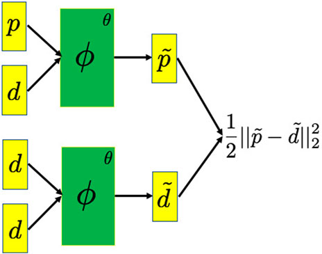
FIGURE 1. Schematic plot of the neural network architecture of the ML-misfit. The predicted data p and measured data d correspond to a single trace of the seismic data in vector form. They are packed to form two inputs, i.e., (p, d) and (d, d). These inputs go through the neural network ϕ with parameters θ, and outputs $\tilde{p}$ and $\tilde{d}$, respectively. The resulting misfit function is defined to be the L2 norm of the difference between the outputs of $\tilde{p}$ and $\tilde{d}$. See Section 2.1 for more information.

Using the form we introduced in Eq. 1, we can verify that the ML-misfit satisfies the following rules for a pseudo-metric:

where p, d, f, q are arbitrary input vectors and, from this point on, we omit the ML-misfit dependency on the neural network parameter θ for brevity. Thus, the resulting ML-misfit guarantees symmetry with respect to the predicted data p and measured data d, and when the predicted data resemble the measured data, the resulting misfit value becomes zero immediately without ever being trained.

We can use CNN and (or) a feedforward neural network for the neural network ϕ; we will describe the details of the neural network parameters for specific problems in Section 3.

2.2 Training the neural network

In this section, we describe how to train the neural network of the ML-misfit defined in Section 2.1 using meta-learning.

In meta-learning, the training dataset is a series of tasks, rather than labeled data in supervised learning problems such as classification. Our loss for the training, referred to as the meta-loss function, is defined as measuring the performance of the current neural network for the implementation of those tasks. Returning to our ML-misfit learning problem, the tasks are formulated by running FWI applications, and the process is the same as conventional iterative waveform inversion, except for replacing the L2-norm misfit (or any other misfit) with a neural network, i.e., the ML-misfit. We run many FWI applications, e.g., using different models. In the training phase, as the true models are available, we define the meta-loss as the normalized L2 norm of the difference between the true model and the inverted one:

where m_k′ denotes the inverted model at step k′ and m_true is the true model. K is the unroll integer, meaning that every K FWI iterations we sum over the model difference as in Eq. 5 and update the neural network parameters of the ML-misfit.

In the training, to update the neural network parameters, we need to figure out the dependency of the meta-loss on the neural network parameters θ. Given model m_k at the current iteration k, we perform the forward modeling to obtain the predicted data p_k. Here, for clarity, we only consider the first-order dependency; i.e., we assume m_k does not depend on the neural network parameters of the ML-misfit and so does the predicted data p_k.

The derivative of the ML-misfit with respect to the predicted data leads to the adjoint source (data residual):

Note that the resulting adjoint source is dependent on the parameter θ of the ML-misfit.

We back-propagate the adjoint source to get the model perturbation:

where ADJOINT denotes the operator for computation of the FWI gradient. Thus, the model can be updated accordingly:

We can easily figure out that the model m_k+1 depends on the neural network parameter θ through the gradient g_k, which further depends on the adjoint source s_k through the gradient computation process, i.e., the operator ADJOINT. Thus, we can accumulate the associated meta-losses given by Eq. 5 for K steps and then compute the gradient with respect to the neural network parameters θ to update these parameters:

where η is the learning rate. The gradient computation is based on automatic differentiation, which is provided in most modern ML frameworks, such as “PyTorch” (which is used in our research and the implementation of the ML-misfit). Eq. 9 represents a standard gradient descent updating scheme. For efficiency and accuracy, we normally adopt more advanced optimization algorithms such as Adam or RMSprop. Those algorithms incorporate moments information for an adaptive learning rate and provide faster convergence for training the neural network, especially when the network is large and deep.

We can only measure the meta-loss at the last FWI iteration step and back-propagate the residual to update neural network parameter. However, for stability consideration, we unroll and accumulate K steps for neural network parameter updating. Initially, we assume that the current model m_k does not depend on the neural network parameters. However, there is actually a high-order dependency between the inverted model and the neural network parameters θ (granted the iteration step is larger than 1, which is normal). In fact, m_k+1 depends on the neural network parameters not only through the gradient ADJOINT(s_k) but also through m_k (we ignore this dependency in our first-order analysis), which further depends on the model m_k−1 and ADJOINT(s_k−1) and so on. This high-order dependency will cause instability, such as gradient explosion in the training process.

Another aspect we need to point out is that the updating of the parameters θ of the neural network requires dealing with high-order derivatives, i.e., the gradient of a gradient. This is because s_k is already the derivative of the ML-misfit (with respect to the predicted data). Updating of the neural network requires the explicit computation of the derivative of the adjoint source s_k with respect to the parameters θ. Most modern ML frameworks include modules for such functions; e.g., in PyTorch, we can use the function “torch.autograd.grad” to deal with this issue.

To better understand the dependency between the models and the neural network parameters, we draw a typical FWI flow using the ML-misfit in Figure 2. The gradient flows for updating the neural network parameter are the blue curves. The red curves correspond to high-order dependency as described above. We also present the pseudo code for training the ML-misfit in Algorithm 1. Note that, in step 20, we detach the current model from the computation graph and this step corresponds to the exclusion of the higher-order dependency between the model and the neural network parameter. Thus, the gradient flow for updating will only follow the blue curves shown in Figure 2.

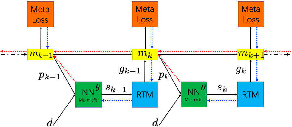
FIGURE 2. Schematic plot describing the flow for the FWI using the ML-misfit function. The green block is the neural network with parameters θ representing the ML-misfit function. The blue block represents the adjoint operator [reverse time migration (RTM) operator]. The red block refers to the computation of the meta-loss defined by Eq. 5. The yellow block denotes the velocity model m_k. p_k is the predicted data modeled by the velocity model and d is the measured datasets. s_k is the adjoint source computed from the ML-misfit. g_k is the gradient output from the RTM block given an adjoint source s_k. The blue and red curves denote the gradient flow for updating parameters θ for the ML-misfit. The blue curves are related to the first-order dependency between the meta-loss and the parameters θ, while the red curves correspond to higher-order dependencies.

In summary, the loss function of Eq. 5 asks the ML-misfit to converge faster with the least model residuals, and this is equivalent to optimization for a cycle-skipping-free objective, as a cycle-skipped model will always correspond to large model residuals. Considering that the ML-misfit already satisfies Eqs 2–4, the optimization based on Eq. 5 will lead to a cycle-skipping-free misfit function and at the same a pseudo-metric (distance) in mathematics. In Section 3, we demonstrate these desirable features of the ML-misfit learned by the machine.

3 Examples

We start with simple travel-time shifted signals, beyond the cycle constraint, to teach the neural network to overcome this limitation of classic misfits. Subsequently, we use a 2D model to teach the neural network to deal with more realistic nonlinearity.

3.1 Developing a convex misfit function for travel-time shifted signals

We normally use shifted signals to evaluate the convexity of a misfit function in FWI. Similarly, in this section, we design a light-weight “FWI” for inverting a single travel-time, which controls the shift in the signal. Based on the proposed meta-learning framework, we teach the ML-misfit to invert such a travel-time shift efficiently. We first share an in-detail description of the setup of the experiment.

3.1.1 Experiment setup

In this example, we propose a simplified FWI to evaluate our method efficiently. In this mini-FWI, we only invert for a single parameter, i.e., the travel-time shift τ. An assumed forward modeling produces a shifted Ricker wavelet representing the predicated data p(t; τ):

where f is the dominant frequency. Eq. 10 leads to a fast simulation of the predicted data p(t; τ) from the travel-time shift parameter τ, which significantly accelerates the testing and evaluation of our methodology.

The meta-loss function of Eq. 5 for training is modified accordingly:

where we omit the summation over multiple steps for brevity (in this example, the unroll parameter K is 5).

In this example, we discretize the waveform of the signal using nt = 128 samples with a sampling interval dt = 0.02 s, and thus simulate a record of length about 2.5 s. In general, the neural network architecture of ϕ in Eq. 1 uses 1D convolutional layers and mimics the AlexNet neural networks (Krizhevsky et al., 2012) in that it uses larger kernels at the earlier convolution layers and smaller kernel sizes with more channels at later layers. In total, we have eight convolution layers. The inputs to the neural network of ϕ are two vectors, i.e., the predicted and measured data of one trace, and they are considered as two channels for the first convolution layer. We follow each convolution layer with a LeakyRelu activation function, followed by MaxPooling. We set the channel numbers to (256, 512, 512, 1024, 1024, 1024, 1024, 2) for the eight convolution layers, while the corresponding kernel sizes are set to (17, 9, 9, 5, 5, 3, 3, 1) with a stride of 1 (we set a relatively large kernel size of 17 for the first convolution layer to accommodate the source signature, because in the training, we use a minimum frequency of 3 Hz whose period is approximately 17 samples for our setup). The kernel and stride size are both set to be 2 for the MaxPooling layer, and thus we halve the length of the data after the MaxPooling operation. Note the last channel number is 2, which indicates outputting a vector of length 2 (which is similar to the mean and variance in the OTMF approach). To keep the output in a specific range, we adopt a Tanh activation function after the last convolution layer. We do not use DropOut or BatchNormalization in our application.

We generate 26,400 true and initial travel times with τ in Eq. 10 ranging between 0.4 s and 2.1 s for training. To inject more variety in the training, we also randomly set the main frequency in Eq. 10 to between 3 Hz and 10 Hz. We invert for 64 travel times, simultaneously. We run 10 iterations for each inversion and set the learning rate for updating the travel-time shift to be 20. We update the neural network parameters every 10 iterations (the unroll parameter K = 10), and the batch size is set to 320. We adopt the Adam algorithm for training the neural network. The learning rate is set to a constant of 1e-6 and we train for 20 epochs. We also create another 6,400 inversion problems for testing. No regularization is used in the training of the ML-misfit. Note that, in the setup described here, the travel-time difference can be as large as 1.7 s, which is clearly far larger than the half cycle of the dominant frequency of 3 Hz. This challenging dataset will drive the ML-misfit to learn to construct a robust misfit to handle such a strong cycle-skipping circumstance.

3.1.2 Results and discussion

Figure 3 shows the curve for the meta-loss (mean value over batch size) of Eq. 11 for the training and testing datasets. Here, we normalize the loss value for the first-epoch training loss to 1. The continuous reduction in the loss for the training shows convergence and demonstrates the success of the training of the ML-misfit neural network. The loss for the testing tasks also becomes rather small, indicating the good generalization property of the trained neural network.

FIGURE 3. Example of the loss over epochs for training the ML-misfit for the travel-time shifted signals. The loss is the squares of the difference between the inverted travel time and the true travel time defined in Eq. 11.

To evaluate the convexity of the ML-misfit with respect to the travel-time shifts, we compute the ML-misfit between a target signal and its shifted version with varying time shifts. In the computation, we choose the main frequency to be 3 Hz, 6 Hz, and 10 Hz, and the travel-time for the target signal is set as 1.25 s, while the time shifts with respect to the target signal vary from −0.85 s to 0.85 s. Figure 4 shows the resulting normalized misfit value for the L2 norm and the ML-misfit. It is obvious that the non-convexity of the L2 norm with respect to time shifts results in local minima, while the machine-learned ML-misfit shows good convexity with respect to time shifts across different frequencies. This indicates that the ML-misfit does learn a more robust way to compare the predicted data and measured data to avoid cycle-skipping. Figure 5 shows the derivates of the misfit function with respect to the travel-time shifts, and such derivatives mimic the gradient in FWI, which is computed via the following equation:

where T denotes transpose operation and F is the misfit function. $\delta p=\frac{\partial F(p,d)}{\partial p}$ is the adjoint source by ML-misfit, and $\frac{\partial p}{\partial \tau }$ is the derivative of the predicted data with respect to the travel-time shift and can be evaluated by Eq. 10. Note that g_τ is a scalar here, as we invert for single time-shift values. From Figure 5, we can see that as expected, the L2 norm shows an incorrect gradient for large time-shift differences, while the ML-misfit gradient always has the correct sign, and the magnitude is in line with the travel-time difference.

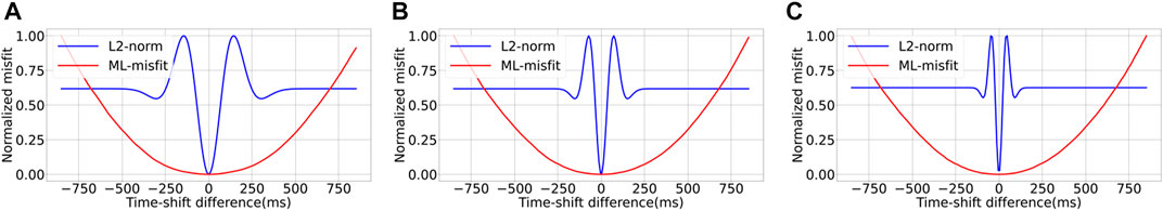
FIGURE 4. Misfit curves for the L2 norm and the ML-misfit with respect to time shifts for data with main frequency (A) 3 Hz, (B) 6 Hz, and (C) 10 Hz.

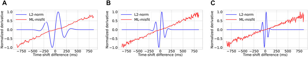
FIGURE 5. Derivatives of the L2 norm and the ML-misfit functions with respect to travel-time shifts for data with main frequency (A) 3 Hz, (B) 6 Hz, and (C) 10 Hz.

To further evaluate the accuracy of the inversion resulting from the ML-misfit function, we show the histogram of the travel-time difference (between the true and inverted travel time) for the testing dataset before and after training in Figure 6. We can see that both the mean and standard deviation are reduced considerably. In Figure 7, we sample and plot 100 true and inverted travel times for the testing datasets. Note that, in this figure, the x-axis (labeled “index”) denotes different experiments, and the y-axis corresponds to the travel time. The ML-misfit inverted travel time shows high accuracy even though the initial travel time is far from the true one, thus indicating a strong cycle-skipping issue (note that the frequency range is between 3 Hz and 10 Hz).

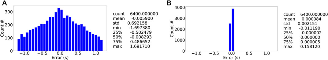
FIGURE 6. Histogram of the travel-time difference between the true and initial travel-time shift inverted by ML-misfit (A) before training and (B) after training.

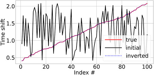
FIGURE 7. Results for 100 true and inverted travel times for the testing dataset for the ML-misfit after training.

Thus, given the setup described in Section 2, we have successfully trained the ML-misfit, and the resulting misfit function shows good convexity with respect to the time shifts. We consider the results obtained and the setup described as the baseline. Subsequently, we test the following aspects to better understand the features of the ML-misfit, and except for the changes specified explicitly below, we use the same setup as the baseline:

• Low-frequency muted: In the training of the baseline model, we input the raw time-shift signals. We may expect that the resulting ML-misfit will learn to filter out the low frequency part of the signal. Thus, we implement a test with input data in which we filter out energy below 2 Hz. We denote this experiment as “low-frequency muted.” In Figure 8, the red curves show the loss for this setup. We can see that, compared to the baseline (black curves), muting low-frequency does not affect the convergence, and this proves that the ML-misfit does learn how to compare the predicted and measured data rather than just perform low-frequency filtering. As expected, the misfit curves over time shifts in Figure 9 also show good convexity.

• Limited training dataset: We know that a ML algorithm is data-hungry, and we need to prepare a proper dataset for training. In this test, as before, we still randomly generate the true and initial travel-time shift to produce the dataset for training. However, we restrict the maximum travel-time shift between the true and shifted signal to be within half a cycle of the dominant frequency. The testing dataset and other setup parameters are the same as before. In Figure 8, the training loss (solid blue) drops quickly, while the testing loss (dotted blue) remains at a high level. This demonstrates the importance of providing a dataset including cycle-skipping features so that the machine can properly learn a robust misfit function.

• Black-box approach: Here, we want to test and prove that our specially designed neural network architecture helps with training convergence. We compare the black-box approach while no special structure is applied to the ML-misfit. For a fair comparison, and to make sure the resulting neural network has a similar number of parameters, we use the function ϕ in Eq. 1 as the ML-misfit, by simply modifying the output of size (i.e., the last channel number) to 1. In Figure 8, the solid green curves show the training loss for this setup. Compared to the baseline, the convergence is slow, and the loss remains at a large value at the end. The convexity of the misfit over time shifts, shown in Figure 9, by the black-box approach is also negatively affected. This experiment further demonstrates the importance of pseudo-metric architecture for the ML-misfit.

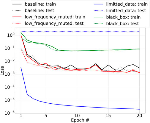
FIGURE 8. Training loss for ML-misfit with different setups.

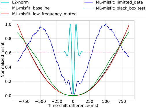
FIGURE 9. Misfit curves for the L2 norm and the ML-misfit trained with different setups. The main frequency is 10 Hz.

The performance of each setup is also reflected in the derivatives with respect to the time difference shown in Figure 10.

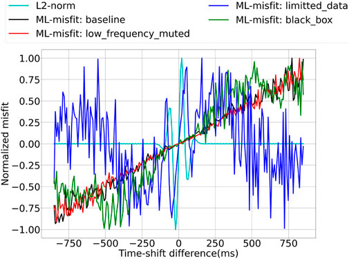
FIGURE 10. Derivatives of the L2 norm and the ML-misfit trained with different setups. The main frequency is 10 Hz.

This simple, while illustrative, travel-time shifted signals example demonstrates that, based on the proposed meta-learning framework, neural networks can learn a cycle-skipping-free misfit function. The introduction of a specific architecture for the misfit function can improve the efficiency of the training as well as the convexity of the resulting misfit function. In Section 3.2, we train the neural network on 2D layered models by running FWI (not a simplified version as in this section) and apply the resulting learned ML-misfit to the Marmousi model.

3.2 The Marmousi model

In this section, we present the result of applying the ML-misfit to the Marmousi model.

As shown in Figure 11B, Marmousi is a complex 2D structural model, and it contains large horizontal and vertical velocity variations. It is a standard benchmark model to evaluate depth-migration and velocity-determination methodologies.

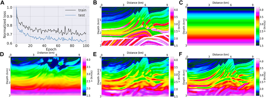
FIGURE 11. Application of the ML-misfit to the Marmousi model: (A) the loss over epochs for training the ML-misfit on the randomly generated 2D model; (B) the true Marmousi model; (C) the initial model for starting the inversion; (D) inversion result for the L2 norm; (E) inversion result for the ML-misfit; (F) inversion result for the L2 norm using (E) as the starting model.

We generate random 2D layered models for training, and these random models are designed to be similar to Marmousi (such as the velocity range, water depth, etc.) while at the same time including randomness. The model size is 3 km in depth and 9 km wide, with a sampling interval of 20 m in both directions, and we mimic a marine geologic setup with velocity ranging from 1,500 m/s to 4,200 m/s. The 2D random layered model is created with a general increase of velocity with depth. Specifically, we randomly create a series of layers z_i with z₀ = 0 km. Thus, the top of the layer i is at depth z_i−1, and the layer bottom is at depth z_i. The interval velocity for layer i is determined by v_i = 1,500 + 1.35ϵz_i, where ϵ is a random number in [0, 1]. To mimic a shallow marine setup and also to stabilize the inversion, we set the first layer of the model to have a water velocity of 1,500 m/s and fix it during the inversion. The water depth for the water layer is also randomly drawn from 100 m to 500 m. With these semi-random velocity models, we utilize the finite-difference method to generate the data. The initial model used to start the FWI is obtained by applying strong smoothing to the true model with a Gaussian smoother of a standard deviation of 2 km.

As the model is a horizontally layered model, we only need to compute a one-shot record to perform the inversion (and a follow-up with summarization over the horizontal direction). We select one shot on the surface with location equals 0. We place 100 receivers evenly spaced at the surface with a maximum offset of 9 km. The recording time is 7.2 s, with 256 samples. We use a 7-Hz central frequency Ricker wavelet (we use the same wavelet both in training and in the application to Marmousi). This is reasonable, as we can usually invert for an accurate wavelet. We mute the energy of the wavelet below 3 Hz, thus guaranteeing that the learned ML-misfit can mitigate cycle-skipping without low frequencies. We perform the FWI based on the pressure wave equation utilizing the full-band data without frequency continuation. Furthermore, we also add total variation (TV) regularization to the model (Alkhalifah et al., 2018; Esser et al., 2018) in the training stage.

In the training stage, we use another 64 models for testing (validation) and, in each epoch, we randomly generate 256 models for training. The neural network architecture of ϕ in Eq. 1 is defined as follows: in total, we have three 1D convolution layers and three fully connected layers. We use MaxPooling after each convolution layer and Tanh as the activation function. The number of channels of the three convolution layers are (128, 256, 512). The kernel size for the three layers is set to (17, 9, 5) correspondingly, and the number of neurons of the fully connected layers are (256, 128, 128).

As shown in Eq. 5, we adopt the L2 norm of the model difference as the meta-loss. We update the parameters of the ML-misfit every 10 FWI iterations (unroll integer K = 10). Thus, given that we have 100 receivers, the batch size for training is 1,000.

We train the neural network for 100 epochs. Figure 11A shows the normalized meta-loss for the training and testing tasks over iterations, the reduction of the loss value suggests the convergence of the training. In Supplementary Figures S1, S2, we show the profiles of the inverted models selected from the testing data using the ML-misfit before and after training. From these profiles, we can see that the inversion of the layered models improves after training, especially for the shallow part of the model. We apply this trained ML-misfit to the modified Marmousi model. Similarly, this Marmousi model extends 2 km in depth and 8 km in distance. We simulate 80 shots and 400 receivers spread evenly on the surface. In order to use the ML-misfit trained on the horizontally layered model, the size of the input must be consistent. Thus, we simulate the record time up to 7.2 s, the same as that used in the training step. Figure 11C shows the initial model for starting the inversion. As before, we perform a full-band inversion (band-passing the data in the frequency range of 3 Hz–7 Hz) without frequency continuation. Figures 11D,E show the inversion results after 150 iterations using the L2 norm and ML-misfit, respectively. The result using an L2 norm shows obvious cycle-skipping artifacts and fails to update the model properly, while the ML-misfit shows considerably improved results with an ability to recover the low-wavenumber components of the model. Taking a smoothed version of Figure 11E as the initial model, we perform FWI for a further 100 iterations using the L2 norm. We obtain the inverted model shown in Figure 11F. Due to the resolved low-wavenumber components of the model for the ML-misfit, the “L2” norm demonstrates its high-resolution features and the resulting model shows high consistency with respect to the true model. The convergence speed of the ML-misfit-based inversion tends to be slightly slower than the conventional “L2”-norm misfit. This is the usual case for any cycle-skipping-free misfit function, as the ML-misfit is trying to find the global solution rather than the local minimum.

4 Discussion

In this section, we dig deeper into the meta-learning framework for learning an ML-misfit and try to explain how the machine learned such an ML-misfit function. To simplify our discussion, we only consider one step of the model updating, assuming a first-order approximation (the initial model m does not depend on the parameters θ of the neural network). Ignoring the normalization term in Eq. 5, we choose the meta-loss as the L2 norm of the difference between the inverted model and true model, i.e., $L=\frac{1}{2}\Vert m-m_{\text{true}}{\Vert }_2^2$. If the adjoint source s computed using Eq. 6 leads to the minimum value (0) for the meta-loss, it should satisfy the following equation:

Here $\mathcal{A}(s)$ denotes ADJOINT(s) in Eq. 7. Without loss of generality, we can reasonably assume that the model-updating step length γ = 1. Furthermore, given that the operator $\mathcal{A}$ defined in Eq. 7 is a linear operator with respect to the adjoint source s, we use ${\mathcal{A}}^{\text{T}}$ to represent its adjoint, i.e., the Born approximation. Thus, the adjoint source, by solving Eq. 10, can be represented as

We observe that one step of first-order meta-learning is equivalent to a supervised learning. Given an initial model m and a true model m_true, such supervised learning takes the input data predicted data p and measured data d, and outputs the adjoint source, which takes the right-hand side of Eq. 14 as its target:

where (x, y) are training data pairs, with x the input and y the target (label), and the mapping function aims to learn $\frac{\partial \mathrm{\Phi }(p,d;\theta )}{\partial p}$.

Note that the term ${({\mathcal{A}}^T\mathcal{A})}^{-1}$ corrects for illumination and resolution while the travel-time information is mostly recovered by ${\mathcal{A}}^T(m-m_{\text{true}})$. Thus, we can deduce that with this kind of supervised learning, the machine tries to learn an adjoint source, which tends to be the Born-modeled wavefield computed from the velocity perturbation corresponding to the difference between the initial and true models. Thus, we provide an intuitive explanation of our meta-learning training strategy using the concept of the supervised learning approach.

5 Conclusion

We have developed a framework for learning a robust misfit function, entitled ML-misfit, for FWI using meta-learning. A specific neural network architecture inspired by the OTMF misfit is suggested, and mathematically, it is strictly a pseudo-metric. The meta-learning approach for training the ML-misfit is a bilevel-optimization problem. The inner optimization is the conventional FWI with the usual human-designed misfit function replaced by the ML-misfit. In contrast, the outer optimization minimizes the meta-loss (which is defined as the difference between the true and inverted models) to update the neural network of the ML-misfit. We have demonstrated that, when trained on randomly generated 1D layered models, the resulting ML-misfit can invert for the Marmousi model free of cycle-skipping using data without frequencies below 3 Hz.

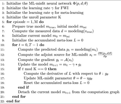
Algorithm 1. Training of the ML-misfit

Plain language summary

In many optimization (inverse) problems such as FWI, the nonlinearity between the model and the corresponding data often causes the inversion process to converge to a local minimum of the optimization rather than a global one, which corresponds to an inaccurate model of the Earth. Often, this situation is alleviated by designing a robust misfit function, which provides a better measurement of the data difference. However, such hand-crafted misfit functions are often ad hoc and require considerable mathematical and physical insights to adapt them to work on a specific dataset. Here, we propose a data-driven misfit function, a method that uses ML to systematically and automatically design the misfit measure for nonlinear inverse problems. This misfit function trained on one-dimensional models performed well on the complex Marmousi model and mitigated the local minimum problem, demonstrating that a machine-learned misfit function is both possible and effective.

Data availability statement

The original contributions presented in the study are included in the article/Supplementary Material; further inquiries can be directed to the corresponding author.

Author contributions

Study conception and design: BS; data collection: BS; analysis and interpretation of results: BS and TA; draft manuscript preparation: BS and TA. All authors reviewed the results and approved the final version of the manuscript.

Acknowledgments

We thank KAUST for supporting the research. The data regarding the Marmousi model is available in Bourlioux et al. (1991). We also show the samples of the data (randomly generated models) in Supplementary Figures S1, S2 for reference.

Conflict of interest

The authors declare that the research was conducted in the absence of any commercial or financial relationships that could be construed as a potential conflict of interest.

Publisher’s note

All claims expressed in this article are solely those of the authors and do not necessarily represent those of their affiliated organizations, or those of the publisher, the editors, and the reviewers. Any product that may be evaluated in this article, or claim that may be made by its manufacturer, is not guaranteed or endorsed by the publisher.

Supplementary material

The Supplementary Material for this article can be found online at: https://www.frontiersin.org/articles/10.3389/feart.2022.1011825/full#supplementary-material

References

Alkhalifah, T., Sun, B., and Wu, Z. (2018). Full model wavenumber inversion: Identifying sources of information for the elusive middle model wavenumbers. Geophysics 83 (6), R597–R610. doi:10.1190/geo2017-0775.1
Andrychowicz, M., Denil, M., Colmenarejo, S. G., Hoffman, M. W., Pfau, D., Schaul, T., et al. (2016). Learning to learn by gradient descent by gradient descent. arXiv:1606.04474.
Araya-Polo, M., Farris, S., and Florez, M. (2019). Deep learning-driven velocity model building workflow. Lead. Edge 38 (11), 872a1–872a9. doi:10.1190/tle38110872a1.1
Araya-Polo, M., Jennings, J., Adler, A., and Dahlke, T. (2018). Deep learning tomography. Lead. Edge 37 (1), 58–66. doi:10.1190/tle37010058.1
Baronian, C., Riahi, M. A., and Lucas, C. (2009). Applicability of artificial neural networks for obtaining velocity models from synthetic seismic data. Int. J. Earth Sci. 98 (5), 1173–1184. doi:10.1007/s00531-008-0314-3
Bleistein, N., Cohen, J. K., and John, W. (2013). Mathematics of multidimensional seismic imaging, migration, and inversion. Springer Science & Business Media.
Bourlioux, A., Bourget, M., Lailly, P., Poulet, M., Ricarte, P., and Versteeg, R. (1991). “Marmousi, model and data,” in Proceedings of the 1990 EAGE Workshop on Practical Aspects of Seismic Data Inversion.
Chebotar, Y., Molchanov, A., Bechtle, S., Righetti, L., Meier, F., and Sukhatme, G. S. (2019). Meta-learning via learned loss. arXiv:1906.05374.
Chen, M., Niu, F., Liu, Q., and Tromp, J. (2015). Mantle-driven uplift of Hangai Dome: New seismic constraints from adjoint tomography. Geophys. Res. Lett. 42 (17), 6967–6974. doi:10.1002/2015GL065018
Cybenko, G. (1989). Approximation by superpositions of a sigmoidal function. Math. Control Signal. Syst. 2 (4), 303–314. doi:10.1007/BF02551274
Engquist, B., and Froese, B. (2014). Application of the Wasserstein metric to seismic signals. Commun. Math. Sci. 9 (11), 979–988. doi:10.4310/CMS.2014.v12.n5.a7
Esser, E., Guasch, L., van Leeuwen, T., Aravkin, A., and Herrmann, F. (2018). Total variation regularization strategies in full-waveform inversion. SIAM J. Imaging Sci. 11 (11), 376–406. doi:10.1137/17m111328x
Fabien-Ouellet, G., and Sarkar, R. (2020). Seismic velocity estimation: A deep recurrent neural-network approach. Geophysics 85 (1), U21–U29. doi:10.1190/geo2018-0786.1
Fichtner, A., and Villaseñor, A. (2015). Crust and upper mantle of the Western Mediterranean – constraints from full-waveform inversion. Earth Planet. Sci. Lett. 428, 52–62. doi:10.1016/j.epsl.2015.07.038
Finn, C., Abbeel, P., and Levine, S. (2017). Model-agnostic meta-learning for fast adaptation of deep networks. arXiv:1703.03400.
Hu, W., Jin, Y., Wu, X., and Chen, J. (2019). A progressive deep transfer learning approach to cycle-skipping mitigation in fwi, 2019. SEG Technical Program Expanded Abstracts, 2348–2352. doi:10.1190/segam2019-3216030.1
Jin, Y., Hu, W., Wu, X., and Chen, J. (2018). Learn low-wavenumber information in FWI via deep inception-based convolutional networks, 2018. SEG Technical Program Expanded Abstracts, 2091–2095. doi:10.1190/segam2018-2997901.1
Krizhevsky, A., Sutskever, I., and Hinton, G. E. (2012). “ImageNet classification with deep convolutional neural networks,” in Advances in neural information processing systems. Editors F. Pereira, C. J. C. Burges, L. Bottou, and K. Q. Weinberger (Curran Associates, Inc.), 25, 1097–1105. Available at: http://papers.nips.cc/paper/4824-imagenet-classification-with-deep-convolutional-neural-networks.pdf.
Lailly, P. (1983). “The seismic inverse problem as a sequence of before stack migrations,” in Conference on Inverse Scattering, Theory and application (Philadelphia, Expanded Abstracts: Society for Industrial and Applied Mathematics), 206–220.
Langer, H., Nunnari, G., and Occhipinti, L. (1996). Estimation of seismic waveform governing parameters with neural networks. J. Geophys. Res. 101 (B9), 20109–20118. doi:10.1029/96JB00948
Maass, P. (2019). “Deep learning for trivial inverse problems,” in Compressed sensing and its applications: Third International MATHEON Conference 2017 (Cham: Springer International Publishing), 195–209. doi:10.1007/978-3-319-73074-5_6
Macías, C. C., Sen, M. K., and Stoffa, P. L. (1998). Automatic NMO correction and velocity estimation by a feedforward neural network. Geophysics 63 (5), 1696–1707. doi:10.1190/1.1444465
Métivier, L., Brossier, R., Mérigot, Q., Oudet, E., and Virieux, J. (2016). Measuring the misfit between seismograms using an optimal transport distance: Application to full waveform inversion. Geophys. J. Int. 205 (11), 345–377. doi:10.1093/gji/ggw014
Nath, S. K., Chakraborty, S., Singh, S. K., and Ganguly, N. (1999). Velocity inversion in cross-hole seismic tomography by counter-propagation neural network, genetic algorithm and evolutionary programming techniques. Geophys. J. Int. 138 (1), 108–124. doi:10.1046/j.1365-246x.1999.00835.x
Ovcharenko, O., Kazei, V., Kalita, M., Peter, D., and Alkhalifah, T. (2019). Deep learning for low-frequency extrapolation from multioffset seismic data. Geophysics 84 (6), R989–R1001. doi:10.1190/geo2018-0884.1
Park, M. J., and Sacchi, M. D. (2020). Automatic velocity analysis using convolutional neural network and transfer learning. Geophysics 85 (1), V33–V43. doi:10.1190/geo2018-0870.1
Pratt, R. G. (1999). Seismic waveform inversion in the frequency domain, part 1: Theory and verification in a physical scale model. Geophysics 64 (3), 888–901. doi:10.1190/1.1444597
Roethe, G., and Tarantola, A. (1991). Use of neural networks for inversion of seismic data. Seg. Tech. Program Expand. Abstr. 1991, 302–305. doi:10.1190/1.1888938
Röth, G., and Tarantola, A. (1994). Neural networks and inversion of seismic data. J. Geophys. Res. 99 (B4B4), 6753–6768. doi:10.1029/93JB01563
Schmidhuber, J. (1987). Evolutionary principles in self-referential learning. on learning now to learn: The meta-meta-meta-hook (Diploma Thesis. Germany: Technische Universitat Munchen. Available at: http://www.idsia.ch/∼juergen/diploma.html.
Shin, C., and Cha, Y. (2008). Waveform inversion in the Laplace domain. Geophys. J. Int. 173 (33), 922–931. doi:10.1111/j.1365-246X.2008.03768.x
Shin, C., and Cha, Y. (2009). Waveform inversion in the Laplace–Fourier domain. Geophys. J. Int. 177 (33), 1067–1079. doi:10.1111/j.1365-246X.2009.04102.x
Sirgue, L., and Pratt, R. G. (2004). Efficient waveform inversion and imaging: A strategy for selecting temporal frequencies. Geophysics 69 (11), 231–248. doi:10.1190/1.1649391
Suárez, J. L., García, S., and Herrera, F. (2019). A tutorial on distance metric learning: Mathematical foundations, algorithms and experiments. arXiv:1812.05944.
Sun, B., and Alkhalifah, T. (2020). ML-descent: An optimization algorithm for full-waveform inversion using machine learning. Geophysics 85 (2), R477–R492. doi:10.1190/geo2019-0641.1
Sun, B., and Alkhalifah, T. (2019b). Robust full-waveform inversion with radon-domain matching filter. Geophysics 84 (5), R707–R724. doi:10.1190/geo2018-0347.1
Sun, B., and Alkhalifah, T. (2019a). The application of an optimal transport to a preconditioned data matching function for robust waveform inversion. Geophysics 84 (6), R923–R945. doi:10.1190/geo2018-0413.1
Sun, H., and Demanet, L. (2019). Extrapolated full waveform inversion with convolutional neural networks, 2019. SEG Technical Program Expanded Abstracts, 4962–4966. doi:10.1190/segam2019-3197987.1
Sun, H., and Demanet, L. (2018). Low-frequency extrapolation with deep learning, 2018. SEG Technical Program Expanded Abstracts, 2011–2015. doi:10.1190/segam2018-2997928.1
Tape, C., Liu, Q., Maggi, A., and Tromp, J. (2009). Adjoint tomography of the southern California crust. Science 325 (5943), 988–992. doi:10.1126/science.1175298
Tarantola, A. (1984). Inversion of seismic reflection data in the acoustic approximation. Geophysics 49 (88), 1259–1266. doi:10.1190/1.1441754
Vilalta, R., and Drissi, Y. (2002). Jun 01) A perspective view and survey of meta-learning. Artif. Intell. Rev. 18 (2), 77–95. doi:10.1023/A:1019956318069
Warner, M., and Guasch, L. (2016). Adaptive waveform inversion: Theory. Geophysics 81 (6), R429–R445. doi:10.1190/geo2015-0387.1
Woodward, M. J., Nichols, D., Zdraveva, O., Whitfield, P., and Johns, T. (2008). A decade of tomography. Geophysics 73 (55), VE5–VE11. doi:10.1190/1.2969907
Wu, Y., Lin, Y., and Zhou, Z. (2018). Inversionet: Accurate and efficient seismic-waveform inversion with convolutional neural networks, 2018. SEG Technical Program Expanded Abstracts, 2096–2100. doi:10.1190/segam2018-2998603.1
Zhu, H., Bozdağ, E., and Tromp, J. (2015). Seismic structure of the European upper mantle based on adjoint tomography. Geophys. J. Int. 201 (1), 18–52. doi:10.1093/gji/ggu492
Keywords: machine learning, full-waveform inversion, misfit function, neural network, unsupervised training
Citation: Sun B and Alkhalifah T (2022) ML-misfit: A neural network formulation of the misfit function for full-waveform inversion. Front. Earth Sci. 10:1011825. doi: 10.3389/feart.2022.1011825
Received: 04 August 2022; Accepted: 05 September 2022;
Published: 29 September 2022.
Edited by:
Mehrdad Soleimani Monfared, Karlsruhe Institute of Technology (KIT), GermanyReviewed by:
Amin Roshandel Kahoo, Shahrood University of Technology, IranKeyvan Khayer, Shahrood University of Technology, Iran
Copyright © 2022 Sun and Alkhalifah. This is an open-access article distributed under the terms of the Creative Commons Attribution License (CC BY). The use, distribution or reproduction in other forums is permitted, provided the original author(s) and the copyright owner(s) are credited and that the original publication in this journal is cited, in accordance with accepted academic practice. No use, distribution or reproduction is permitted which does not comply with these terms.
*Correspondence: Bingbing Sun, bingbing.sun@kaust.edu.sa