An Investigation of Rainfall-Induced Landslides From the Pre-Failure Stage to the Post-Failure Stage Using the Material Point Method

Introduction

Rainfall-induced landslides have been a challenge for many decades. Leroueil (2001) indicated the complex relationships existing between rainfall conditions, pore water pressure, soil strength, safety factors, and movement rates. Leroueil (2001), Calvello et al. (2008), and Cascini et al. (2010) stated that rainfall-induced landslides evolve with the complexity of hydro-mechanical responses in the pre-failure, failure, and post-failure stages. Picarelli et al. (2004) depicted a schematic of slope behavior to that indicated that the characteristics of soil displacement behave differently in different stages, as shown in Figure 1. In the pre-failure stage, the soil moves at a constant rate, and it occurs together with local failure, such as the development of shear zones (Cascini et al., 2014). Afterwards, a continuous shear surface (slip surface) will form through the entire soil mass, which leads to the failure stage (Leroueil and Picarelli, 2012; Cascini et al., 2014). In the post-failure stage, the dynamic behavior of soil mass exhibits different types of movement, including slide, spread, and flow (Leroueil and Picarelli 2012). Many approaches have been proposed to relate these relationships in different combinations using both statistically-based models and physically-based models (Cascini et al., 2010). Cuomo (2020) reviewed a wide body of literature on the topic and concluded that a numerical model is the most efficient way to understand the complexity of rainfall-induced landslides.

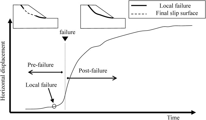
FIGURE 1. Schematic of slope behavior (modified from Picarelli et al., 2004).

The applicability of various numerical methods for landslide modeling has been compared and discussed by Bandara et al. (2016), Soga et al. (2016), Cuomo (2020), and Yuan et al. (2020). Yuan et al. (2020) mentioned that the finite element method (FEM) can be used to automatically detect the shape and location of slip surfaces instead of the limit equilibrium method (LEM). However, the nodal displacement can increase significantly, accompanied by the failure and post-failure stages, as shown in Figure 1, where severe mesh distortions result in simulation non-convergence (Bandara et al., 2016; Soga et al., 2016; Yuan et al., 2020). Thus, Bandara et al. (2016) and Soga et al. (2016) suggested that the post-failure stage be simulated independently using different numerical methods, for example, the finite difference method (FDM) with a depth-integrated model. Accordingly, the numerical parameters and results cannot be expected to have a good consistency in the pre-failure, failure, and post-failure stages. In order to overcome the aforementioned problems, Soga et al. (2016) suggested that the mesh-free technique may be a solution. The technique includes smooth particle hydrodynamics (SPH), the material point method (MPM), the particle finite-element method (PFEM), the finite-element method with Lagrangian integration points (FEMLIP), and the element-free Galerkin (EFG) method. In particular, many researchers have applied the material point method for the simulation of rainfall-induced landslides in recent decades (Yerro et al., 2015; Bandara et al., 2016; Soga et al., 2016; Wang et al., 2018; Lee et al., 2019a; Lee et al., 2019b; Ceccato et al., 2019; Cuomo et al., 2019; Lei et al., 2020; Liu et al., 2020; Martinelli et al., 2020; Liu and Wang, 2021; Nguyen et al., 2021).

The investigation of the development of rainfall-induced landslides using the material point method has been remarkably successful in the past decade. In order to model soil-water-structure interaction, Al-Kafaji (2013) and Jassim et al. (2013) proposed a coupled 2-phase 1-point MPM formulation for saturated soil, and a frictional contact algorithm was developed to simulate the interaction between a structure and soil. With the help of their contribution, the coupled 2-phase 1point MPM formulation was applied to simulate the post-failure stage of a rainfall-induced landslide assuming that a phreatic surface existed before slope failure and the effect of suction was minor as soil deformation increased (Lee et al., 2019a; Cuomo et al., 2019; Nguyen et al., 2021). Yerro et al. (2015) attempted to model infiltration in an unsaturated brittle material, where a coupled 3-phase 1-point MPM formulation associated with a suction-dependent elastoplastic Mohr-Coulomb model was proposed; the well-known van Genuchten model was applied, and the rainfall boundary conditions only considered the type of pore water pressure. Later, different pseudo-3-phase 1-point MPM formulations were proposed by Bandara et al. (2016), Wang et al. (2018), Lee et al. (2019b), Martinelli et al. (2020), and Ceccato et al. (2020). Bandara et al. (2016) derived a coupled pseudo-3-phase 1-point MPM formulation and obtained the infiltration rate of rainfall boundary based on Darcy’s velocity. Other researchers derived a coupled pseudo-3-phase 1-point MPM formulation associated with true liquid velocity, and different algorithms for the infiltration rate of rainfall boundary were proposed by Martinelli et al. (2020) and Ceccato et al. (2019). The former implemented it in a linear unsaturated model and benchmarked it in a one-dimensional soil column test (Martinelli et al., 2020). The latter perform it using the van Genuchten model and benchmarked it in a two-dimensional levee test (Ceccato et al., 2020). Accordingly, a physical-based model using the material point method can be an appropriate solution to investigate the dynamic behavior of rainfall-induced landslides.

This study began the investigation with lab-scale rainfall-induced slope failure, which was implemented by Moriwaki et al. (2004) in Japan. This is a classic experiment and has been studied using different numerical models (Ghasemi et al., 2019; Nguyen et al., 2021; Yang et al., 2021). However, the deformation characteristics influenced by the rainfall conditions can only be investigated in the pre-failure stage or in the post-failure stage, separately. Yang et al. (2021) applied a numerical model based on the finite element method, so the deformation characteristics could only be investigated before the post-failure stage. Ghasemi et al. (2019) and Nguyen et al. (2021) used a different numerical model, which was developed with a 2-phase 1-point MPM formulation, but a rainfall boundary condition algorithm was not available in their model. Hence, the process of infiltration had to be omitted in their studies, and they could only investigate the deformation characteristics in the post-failure stage. In order to improve the previous limitations, this study proposed a numerical model, which implemented a pseudo-3-phase 1-point MPM formulation, to simulate the lab-scale rainfall-induced slope failure. This study applied the rainfall boundary condition algorithm following Martinelli et al. (2020) to validate the van Genuchten model. Therefore, the deformation characteristics influenced by the rainfall conditions could be completely investigated from the pre-failure stage to the post-failure stage.

With help of the proposed model using MPM, this study was able to provide a further investigation on the effect of rainfall. Yang et al. (2021) investigated the effect of rainfall only in the pre-failure stage and did not discuss the location of rising pore water pressure against varying rainfall intensities. Ghasemi et al. (2019) and Nguyen et al. (2021) investigated post-failure behavior without considering the effect of rainfall due to the limitations inherent in their numerical model. Therefore, variations in the rainfall intensity corresponding to the pattern of rising pore water pressure and slope failure can be discussed in this study.

The paper is organized as follows: Theory and Numerical Algorithm presents the theory and numerical algorithm for the coupled pseudo-3-phase 1-point MPM formulation, as well as the rainfall boundary conditions. Then, the numerical simulation of the lab-scale rainfall-induced slope failure, as described in Moriwaki et al. (2004), is described in Numerical Simulation of a Lab-Scale Rainfall-Induced Slope Failure. Finally, the parametric study is discussed in Parametric Study. The proposed numerical algorithm makes it possible to investigate a rainfall-induced landslide from pre-failure stage to post-failure stage, and it offers a further understanding of the effect of rainfall intensity on dynamic soil behavior. According, the findings from this study may provide guidance for geo-environmental risk assessment.

Theory and Numerical Algorithm

Governing Equations

A natural slope can be considered to be a media structured in the form of three phases (solid, liquid, and gas). In this study, a coupled pseudo-3-phase 1-point MPM formulation is derived assuming the gas phase is ignored in the governing equations. Thus, the mass exchange of air and water between the liquid and gas phases are also ignored, and the air pressure is set to zero. The subscripts s and l denote solid and liquid phases (ph), respectively. The subscript m indicates the mixture. The summation of the volume of the solid phase (${\mathit{V}}_{\mathit{s}}$) and the volume of the voids (${\mathit{V}}_{\mathit{void}}$) is equal to the total volume ($\mathit{V}$). ${\mathit{V}}_{\mathit{void}}/\mathit{V}$ indicates the porosity ($n$). Since the volume of liquid is $V_l$, ${\mathit{V}}_{\mathit{l}}/{\mathit{V}}_{\mathit{void}}$ indicates the degree of saturation (${\mathit{S}}_{\mathit{l}}$). ${\rho }_l$ and ${\rho }_s$ indicate the density of the liquid phase and solid phase, repectively. The density of the mixture phase (${\rho }_m$) is determined by the volume fraction and the true density of each phase, i.e., ${\rho }_m=\left(1-n\right){\rho }_s+n{\rho }_l$.

The following general assumptions are adopted

• Isothermal conditions

• No mass exchange between solid and liquid

• Solid grains are incompressible

• Smooth distribution of $n$ and $S_l$ in the soil

• Small spatial variations in the water mass

The momentum balance of the liquid phases is given as .

where the vector ${\mathit{a}}_l$ is the acceleration of the liquid; $p_l$ is the liquid pressure, and $\mathit{b}$ is the body force vector. The third term in right hand side is the drag force corresponding to Darcy’s law, where ${\mu }_l$ is the dynamic viscosity of the liquid, and $k_l$ is the intrinsic permeability of the solid skeleton. ${\mathit{v}}_{\mathit{l}}$ and ${\mathit{v}}_s$ indicate the velocity fields for the liquid and solid phases, respectively. The relative permeability $k_{rel}$ is given by a saturation function, which is equal to 1 for fully saturated soil and decreases with the degree of saturation. In (1), $\mathit{n}{\mathit{S}}_{\mathit{l}}\left({\mathit{v}}_{\mathit{l}}-{\mathit{v}}_{\mathit{s}}\right)$ is called as the seepage velocity (or Darcy’s velocity) ($\mathit{w}$). With help of Eq. 1, Martinelli et al. (2020) yielded the momentum balance of the mixture as :

where the vectors ${\mathit{a}}_{\mathit{m}}$ and ${\mathit{a}}_{\mathit{s}}$ are the acceleration of the mixture and solid phases, respectively. $\mathit{\sigma }$ is the total stress tensor of the mixture, and $\mathit{I}$ is unit stress tensor.

The expression for the mass balance of solid phase is under the third and fourth points of the general assumption, and it can be written as

For the mass balance of the liquid phase, barotropic behavior is assumed for the fluid, and so the time derivative of the liquid density ($\partial {\mathit{p}}_{\mathit{l}}/\partial \mathit{t}$) is thus considered to be related to the time derivative of the pore water pressure ($\partial {\mathit{p}}_{\mathit{l}}/\partial \mathit{t}$) (Wang et al., 2018). When the soil is partially saturated, the air pressure ($p_a$) is assumed to be zero, where $p_a-p_l$ indicates the suction ($s$). Thus, the time derivative of the degree of saturation ($\partial {\mathit{S}}_{\mathit{l}}/\partial \mathit{t}$) can be the function of $\partial {\mathit{p}}_{\mathit{l}}/\partial \mathit{t}$ (Wang et al., 2018). Under these assumptions, the mass balance of liquid phase can be expressed as

where $K_l$ is the bulk modulus of the liquid. $\partial {\mathit{S}}_{\mathit{l}}/\partial \mathit{s}$ represents the specific moisture capacity (Zienkiewicz et al., 1990).

The relationships among ${\mathit{S}}_{\mathit{l}}$, $s$, and ${\mathit{k}}_{\mathit{rel}}$ are important when attempting to model the behavior of unsaturated soil. The soil-water retention curve (SWRC) for the van Genuchten model is given as follows:

where $p_0$ is the air-entry pressure (unit of kPa); $\lambda$ is an empirical parameter, and $S_{max}$ and $S_{min}$ are respectively the degree of saturation at full saturation and under very dry conditions. The hydraulic conductivity curve (HCC) can be summarized as follows:

where $S_e$ is the effective saturation (Mualem, 1976). $\partial S_l/\partial s$ can be computed by

For the mechanical constitutive equation, the concept of Bishop is introduced to express the effective stress of unstated soil ($\mathrm{\sigma }\text{'}$), which is equal to $\mathrm{\sigma }-S_l{p}_l\mathit{I}$. The incremental effective stress ($\text{d}\mathrm{\sigma }\text{'}$) is associated with the strain increment vector ($\text{d}\mathit{\epsilon }$) and can be presented as $\text{d}\mathrm{\sigma }\text{'}=\mathrm{D}\text{d}\mathit{\epsilon }$, where $\mathrm{D}$ is the tangent matrix. The stress-strain relationship is measured using the Jaumann stress rate, and the material time derivative of the Cauchy stress tensor is written as $\text{d}\mathrm{\sigma }\text{'}=\mathrm{D}\text{d}\mathit{\epsilon }+\mathrm{\sigma }\text{'}{\mathrm{W}}^{\mathrm{T}}-\mathrm{W}\mathit{\sigma }\mathit{\text{'}}$, where $\mathrm{W}$ is the vorticity. In this paper, the elastoplastic model with the Mohr-Coulomb failure criteria is used (Bandara and Soga, 2015; Ceccato et al., 2019).

Discretization and Material Point Method Algorithm

Discretization of Material Point Method

Numerically implementing our proposed governing equations was accomplished using the material point method. As visualized in Figure 2, a set of material points (MPs) discretized the material domain and carried all information, including density, strain, stress, velocity, and other material parameters (Al-Kafaji, 2013; Zhang et al., 2016). The MPs represent the continuum body and move through an Eulerian background grid (Zhang et al., 2016; Martinelli et al., 2020). The fixed Eulerian grid structured by the node, the node was used to determine the divergence terms and spatial gradient, and no historical information was carried inside the node (Zhang et al., 2016). In order to map the material’s information from the MPs to a node or from a node to an MP, as show in Figures 2A,C, the linear shape function was used to assemble MPs or nodes as in the finite element method. $N^p$ and $N^n$ indicate the linear shape functions of MPs and nodes, respectively. The position of any node and material point can be denoted by

where $x^n$ and $x^p$ indicate the material information, $x=\text{x}, v,a$ for position, velocity, and acceleration, respectively. $i$ is a series number with spatial discretization. The gradient of the linear shape function is represented as $\nabla N^p$ and $\nabla N^n$.

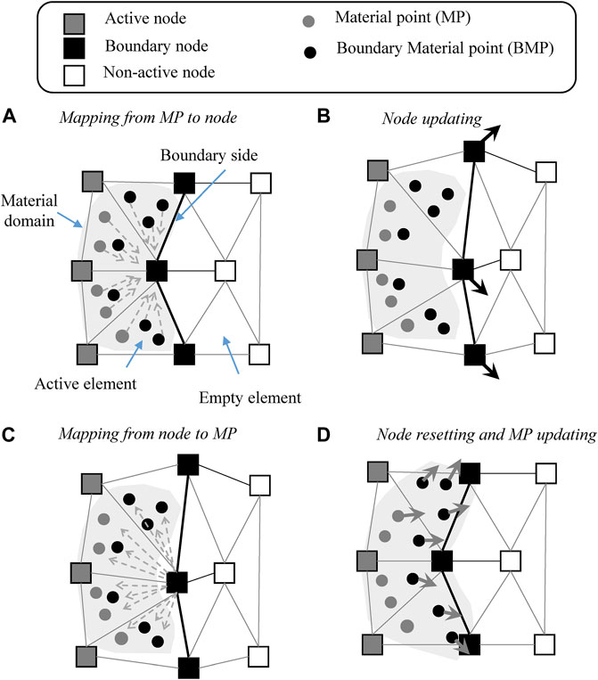
FIGURE 2. Schematic of the material point method. (A) Mapping from MP to node. (B) Node updating. (C) Mapping from node to MP. (D) Node resetting and MP updating.

In the discretized equations, Equations 1, 2 can be presented in a weak form as follows:

where ${\mathit{a}}_l^n$ , ${\mathit{a}}_s^n$ , ${\mathit{v}}_l^n$ and ${\mathit{v}}_s^n$ are nodal acceleration and velocity vectors. ${\tilde{\mathit{M}}}_l^n$ and ${\mathit{M}}_s^n$ are the lumped mass matrix of liquid and solid at the nodes. ${\mathit{F}}_l^{ext}$ , ${\mathit{F}}_l^{grav}$ , ${\mathit{F}}_l^{int}$ , ${\mathit{F}}_s^{ext}$ , ${\mathit{F}}_s^{grav}$ , and ${\mathit{F}}_s^{int}$ are the internal nodal force, gravity nodal force, and external nodal force vectors for each phase, respectively. ${\mathit{Q}}_l^n$ and ${\mathit{Q}}_m^n$ are the drag force matrices for each phase at the nodes. In this paper, the nodal information in Eqs 10, 11 can be calculated following Al-Kafaji (2013).

An explicit Euler method is applied to integrate the model equations in time. Meanwhile, the velocities and positions of each phase could be updated respectively with the accelerations and velocities of each phase as follows:

The Material Point Method Time Marching Procedure

The MPM scheme in this study follows modified update-stress-last (MUSL) scheme (Sulsky et al., 1995). A single computational cycle of numerical algorithm is described as follows:

(I). The discrete MP information is known at time $t^k$. The initialized variables for the solid phase include ${\text{x}}_s^{p,k}$, ${\mathit{v}}_s^{p,k}$, $\mathrm{\sigma }{\text{'}}^{p,k}$, $n^{p,k}$, $V^{p,k}$, and ${\rho }_s$. For the liquid phase, the initialized variables include ${\mathit{v}}_l^{p,k}$, $S_l^{p,k}$, $p_l^{p,k}$, $K_l^{p,k}$, ${\mu }_l$, $k_l$, $k_{rel}^{p,k}$, and ${\rho }_l$ The linear shape function ($N^{p,k}, N^{n,k}$) and the gradient of the linear shape function ($\nabla N^{p,k}, \nabla N^{N,k}$) can be associated with the position of the solid’s MP (${\text{x}}_s^{p,k}$) and the grid background.

(II). The liquid acceleration node (${\mathit{a}}_l^{n,k}$) is determined using Eq. 10. The solid acceleration node (${\mathit{a}}_s^{n,k}$) is determined by Eq. 11. Because the concept of Bishop effective stress is used, the total stress ${\mathrm{\sigma }}^{p,k}$ equals to $\mathrm{\sigma }{\text{'}}^{p,k}+S_l^{p,k}{p}_l^{p,k}$. The second step can be visualized in Figures 2A,B.

(III). The MP velocities for each phase at the new time $k+1$ are updated using the nodal accelerations for each phase, as shown in Figure 2C. With help of Eq. 12, the formula reads as

Because the nodal momentum of each phase can be estimated using the material point masses and velocities, the nodal velocities at the new time $k+1$ are finally computed as the ratio between the nodal momentum and the nodal mass. The computation is as follows:

(IV). The strain rates of each phases at the MPs is shown as ${\dot{\epsilon }}^{p,k}=\Delta {\epsilon }^{p,k}/\Delta t$. These can be determined using the nodal velocity of each phases as follows:

(V). The updating of the MP’s effective stress at the new time ($\mathrm{\sigma }{\text{'}}^{p,k+1}$) is associated with the strain increment of the solid phase ($\Delta {\epsilon }_s^{p,k}=\Delta t{\dot{\epsilon }}_s^{p,k}$) and the vorticity of the solid phase (${\mathrm{W}}_s^{p,k}$). The stress-strain relationship is adopted using the Jaumann stress rate as follows:

The failure criteria follow the standard Mohr-Coulomb model.

(VI). The increment of the pore water pressure ($\Delta p_l^{p,k}$) at a given material point is calculated according to (4) and can be presented as follows:

where $s_l^{p,k}=-p_l^{p,k}$. The specific moisture capacity ($\partial S_l^{p,k}/\partial s_l^{p,k}$) is obtained using Eq. 9. Then, the pore water pressure is updated using $p_l^{p,k+1}=p_l^{p,k}+\Delta p_l^{p,k}$.

(VII). The MP’s degree of saturation ($S_l^{p,k+1}$) and relative permeability ($k_{rel}^{p,k+1}$) then update in this step. When the updating results in a pore water pressure ($p_l^{p,k+1}$) larger than zero, $S_l^{p,k+1}$ updates using Eq. 5. Then, $k_{rel}^{p,k+1}$ updates based on $S_l^{p,k+1}$ using Eqs. 6, 7.

(VIII). The other MP information then updates at this step. The updating volume of the solid phase at MP is described as $V_s^{p,k+1}=V_s^{p,k}\left[1+tr\left(\Delta {\epsilon }_s^{p,k}\right)\right]$. The MP’s position at the solid phase is updated using the nodal velocity of solid phase as follows:

(IX). Finally, the information for the material points at the new time $k+1$ is carried for the next step, and the mesh nodes are initialized as shown in Figure 2D.

Treatment of the Boundary and Initial Conditions

In order to deal with boundary conditions in the material point method, the boundary node, boundary side, and boundary material point have to be determined, as shown in Figure 2. (Bandara et al., 2016; Ceccato et al., 2020; Martinelli et al., 2020). A schematic of the boundary treatment is depicted in Figure 3. For the displacement and contact surface boundaries, prior to the calculation, the boundary node and the boundary side have to be assigned. For the rainfall boundaries, the boundary node and boundary side are detected using the active element and the empty element at each time step. The active element and the empty element are identified by the location of the MPs. When the material point is adjacent to the boundary side, it is defined as the boundary material point.

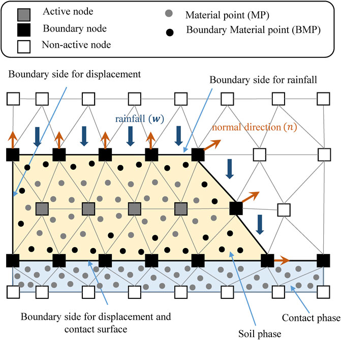
FIGURE 3. Schematic of the boundary treatment.

In a case of a fully fixed node, the nodal velocities and accelerations are set to zero (Al-Kafaji, 2013), so the specified values at the boundary node will not update in the computational cycle. Along a contact surface, the nodal velocities are adjusted to avoid interpenetration and to have tangential forces compatible with the Coulomb’s friction criterion (Al-Kafaji, 2013). The solid phase nodal accelerations (${\mathit{a}}_s^{n,k}$) along a specific contact surface are adjusted according to the given friction coefficient after the computational cycle carried out in the second step (II).

In a case under rainfall conditions, this paper follows the study of Martinelli et al. (2020). When the prescribed seepage velocity is known, i.e., rainfall intensity (mm/hr), the nodal accelerations of each phase (${\mathit{a}}_s^{n,k}$, ${\mathit{a}}_l^{n,k}$) are adjusted in order to comply with the rainfall data after the computational cycle in the second step (II). The description about the correction of nodal acceleration is following Martinelli et al. (2020), and has been written in the first section of Supplementary Material. The validation of the rainfall boundary condition is mentioned in the second section of Supplementary Material. When the prescribed pore water pressure is specified, it is applied to the boundary material point (BMP) directly, and the pore water pressure will not update in the computational cycle in the sixth step (VI).

In the treatments that take place in the initial condition, the initial state is assumed to be satisfied with geostatic and hydrostatic conditions, and so the initial velocities of each phase can be set as zero (Bandara et al., 2016; Siemens, 2018). The initial stress distribution is set using a $K_0$ procedure (Bandara et al., 2016). The initial pore water pressure distribution is given corresponding to the phreatic surface, and the phreatic line can be defined by users. Above the phreatic surface, the suction is generated hydrostatic until it reaches a prescribed value. Below the phreatic surface, the pore water pressure is generated according to the depth of the groundwater (Siemens, 2018).

Numerical Simulation of a Lab-Scale Rainfall-Induced Slope Failure

The proposed model was used to simulate an experiment involving a lab-scale rainfall-induced slope failure (Figure 4), which was originally performed by Moriwaki et al. (2004). The steel flume was 23 m long, 7.8 m high, 3 m wide, and 1.6 m deep, as shown in Figure 4B. The model was composed of four segments with different lengths and inclinations. The first one, located at the toe, was horizontal and 6-m-long; the second one was 6-m-long 10° inclined segment; the third one was a 10-m-long 30° segment, and the final one was horizontal and 1 m long. The flume was filled with loose Sakuragawa River sand with a uniform depth of 1.2 m. Instruments were installed with five surface displacement meters (D-1 to D-5), fifteen pore-water pressure gauges (KP-01 to KP-15), and eleven piezometers (G-1 to G-11), as shown in Figure 4B. A constant intensity of rainfall at 100 mm/h (≈2.78 × 10⁻⁵ m/s) was sparked, as shown in Figure 4A. About 6,300 s after the start of the rainfall, the piezometers recorded rising pore-water pressure linearly, and a rapid movement of soil was triggered at 9,267 s. The evolution of the pore water pressure is shown in Figure 4C. The distribution of deformation after the slide stopped is depicted in Figure 4D.

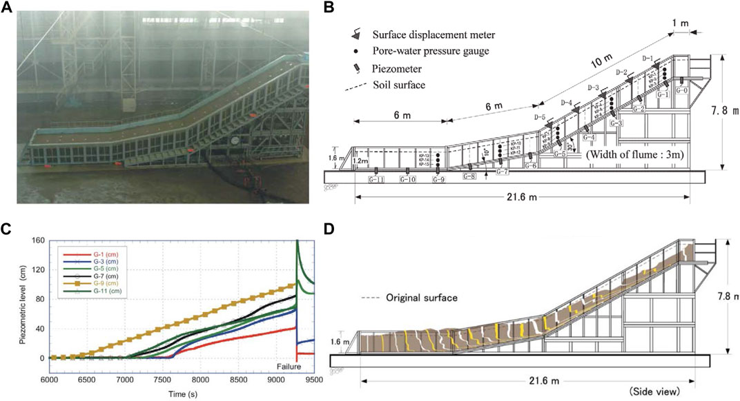
FIGURE 4. The of rainfall-induced slope failure experiment (Moriwaki et al., 2004): (A) Model configuration during the experiment; (B) The setup for the steel flume and the location of the sensors; (C) The piezometer record before the slope failure (D) Material deformation after the slope failure.

The configuration in simulation for the experiment of rainfall-induced slope failure is depicted in Figure 5. The computational domain ranged from $x=0\text{ m}$ to $x=21.6\text{ m}$ and $y=-1 \text{m}$ to $y=8\text{ m}$, with a element size of 0.25 m. In total, 9,925 elements and 3,226 nodes were used. For each element, eight particles were specified. The soil phase was given according to the geometry of the soil layer, and it was located on a contact phase defined as a rigid body. A contact surface was located at the interface between the soil phase and the contact phase. For the assignment of the boundary conditions, two side and bottom boundaries for the contact phase were given as a type of fixed displacement condition, and two side boundaries for the soil phase were set as a type of roller displacement. For the rainfall boundary condition, a constant intensity of rainfall was equal to 3 × 10⁻⁵ m/s and was indicated at soil surface phase. For the initial condition, the initial stress field was generated using a $K_0$ procedure, and the suction was generated hydrostatically from the impervious layer. Following the parametric study of Yang et al. (2021), it was assumed that the maximum suction was not over 10 kPa.

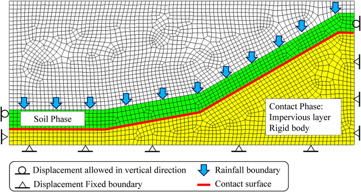
FIGURE 5. Configuration in the simulation of a rainfall-induced slope failure.

The material parameters for the soil phase are given in Table 1. The size of solid grain and porosity density directly followed Moriwaki et al. (2004). Yang et al. (2021) carried out a parametric study using various hydrological factors, i.e., a soil-water retention curve (SWCC) and a hydraulic conductivity curve (HCC), and their suggested parameters were used in this study. Ghasemi et al. (2019) and Nguyen et al. (2021) also did a parametric study using various geological factors, i.e., the Young’s modulus, and friction angle, etc., and this study followed their suggestions for the Young’s modulus, friction analge.

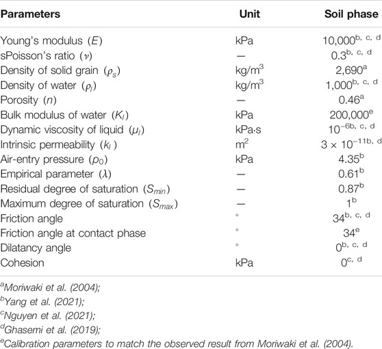
TABLE 1. Material parameters for the rainfall-induced slope failure.

The proposed model was validated against the experimental results. The measurements and simulations of the pore water pressure were generally in acceptable agreement. The comparison is shown in Figure 6. Moriwaki et al. (2004) reported that the measured pore water pressure (PWP) at G-9 rose earlier than at G-5 by about 1,000 s. The measured rising speed of the PWP at G-9 and G-5 were about 3.4 × 10⁻⁴ m/s and 3.7 × 10⁻⁴ m/s, respectively. According to Figure 6A, the proposed model predicted that the time interval between the rise in the PWP between G-9 and G-5 was about 800 s. The speed at which the PWP rose at locations G-9 and G-5 were estimated to be lower by about 24 and 20%, respectively. In terms of the verification of the cumulative surface displacement, the observed and simulated evolutions of cumulative surface displacement at D-1, D-3, and D-5 are depicted in Figure 6B. Moriwaki et al. (2004) reported that the slope failure occurred suddenly and the elapsed time was approximately 6 s. The maximum cumulative surface displacements were measured to be between 3 and 3.7 m. In the simulation, the elapsed time for the slope movement was approximately 10 s, and the maximum cumulative surface displacements were estimated to be between 4.3 and 5 m. At D-5, the measured and simulated velocity of soil movement were consistent during the elapsed time of 0–5 s. However, the sliding velocity simulations at D-1 and D-3 were estimated to be lower than the measured results. Moriwaki et al. (2004) found that the soil filled the flume at a relative density of 3%, and the deformation was accompanied with a mix of compaction and shear. It was felt here that the proposed model using the standard Mohr-Coulomb model might not be a suitable option to simulate post-failure behavior of lab-scale rainfall-induced slope failure. In short, the proposed model using MPM exhibited better performance than that found in a previous study, in which the evolution of the pore water pressure during infiltration could be investigated and improvements in the soil deformation simulation were achieved.

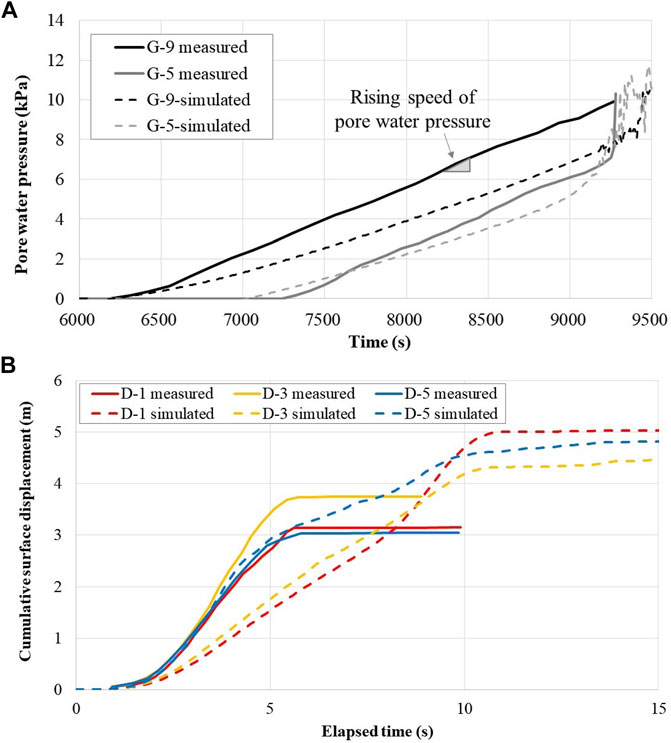
FIGURE 6. Comparison of the measured and simulated results: (A) Evolution of pore water pressure at G-5 and G-9; (B) Evolution of cumulative surface displacement at D-1, D-3, and D-5.

Parametric Study

In the parametric study, the effect of rainfall intensity on the rising pore water pressure and dynamic soil behavior characteristics were evaluated. With help of the proposed model using MPM, variations in the rainfall intensity corresponding to the pattern of rising pore water pressure and slope failure can be discussed in this section.

The ratio of $I/k_s$ was introduced by Yang et al. (2021) and applied to investigate the magnitude of the rainfall effect. Accordingly, the ratio of rainfall intensity ($I$) to hydraulic conductivity ($k_s$) is sensitive to the time required to increase the time and speed of PWP changes in the bottom soil layer ($v_{\text{PWP}}$). Hence, the $I/k_s$ ratio was applied in the parametric study. Seven values of rainfall intensity (I) were used in the parametric study. According to Table 1, the hydraulic conductivity (k_s) equaled 3 $\text{x}{10}^{-4}$m/s, corresponding to the intrinsic permeability ($k_l$) and dynamic viscosity of liquid (${\mu }_l$) values. Because I was normalized by k_s, the seven values could be presented as $I/k_s=1$, $I/k_s=0.75$, $I/k_s=0.5$, $I/k_s=0.25$, $I/k_s=0.1$, $I/k_s=0.75$, and $I/k_s=0.67$. The lab-scale rainfall-induced slope failure was simulated with the seven different rainfall intensities, and the other parameters were kept at the given values, as shown in Table 1.

Effect of Rainfall on Changes in the Pore Water Pressure

The ratio of the various rainfall intensities against the speed at which the pore water pressure rose at G-5 and G-9 is depicted in Figure 7A. The speed of the rise in pore water pressure ($v_{\text{PWP}}$) was divided by the hydraulic conductivity ($k_s$), and the $v_{\text{pwp}}/k_s$ ratio was introduced to present the intensity of the speed at which the pore water pressure rose. An interesting finding was that the increasing $I/k_s$ ratio caused dramatic response in the form of the growth in the $v_{\text{pwp}}/k_s$ ratio. In the case of $I/k_s=0.1$, the $v_{\text{pwp}}/k_s$ ratios at G-9 and G-5 were 0.85 and 0.99, respectively. This means that speed at which the PWP rose was close to the hydraulic conductivity when the rainfall intensity was relatively small. In the case of $I/k_s=0.1$, the $v_{\text{pwp}}/k_s$ ratios at G-9 and G-5 reached 18.9 and 20.7, respectively. This means that a sudden increase in pore water pressure can be caused by high intensity rainfall.

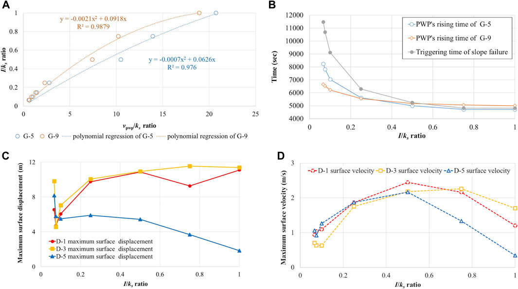
FIGURE 7. Effects of rainfall intensity on a rainfall-induced landslide: (A) changes in the $v_{\text{PWP}}/k_s$ ratio; (B) changes in the time at which the PWP rose and the time at which slope failure was triggered; (C) changes in the maximum surface displacement; (D) changes in the maximum surface velocity.

A further investigation on the effects of variations in rainfall intensity on the amount of time required for the pore water pressure rise was carried out, the results of which are plotted in Figure 7B. The locations where pore water pressure rose preferentially varied with the rainfall intensity. Accordingly, a schematic of the changes rainfall-induced pore water pressure is shown in Figure 8. When the $I/k_s<0.5$, the simulation indicated that a unsaturated wetting front developed from the ground surface and moved forward to the bottom soil layer, as shown in Figure 8A-i. After the wetting front reached the bottom soil layer, as depicted in Figure 8A-ii, ground water was generated from the lowest location on the slope. Hence, the time required for the pore water pressure to rise at G-9 was earlier than that at G-5, as shown in Figure 7B. When the $I/k_s>0.5$ in the simulation, a wetting front with high degree of saturation developed, as shown in Figure 8B-i. With the help of the higher intensity rainfall, the forward speed of the wetting front was faster. As shown in Figure 8B-ii, the wetting front reached G-5 earlier than G-9, but the difference in the time required for the PWP to rise at G-5 and G-9 was very small. After the wetting front reached the bottom soil layer, as depicted in Figure 8B-iii, the soil layer was close to a fully saturated condition. The different characteristics of the rainfall-induced pore water pressure resulted in different types of post-failure behavior. This implied that the ratio of $I/k_s$ is a very important index to distinguish the type of slope failure.

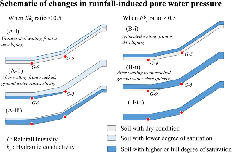
FIGURE 8. Schematic of changes in rainfall-induced pore water pressure.

Effect of Rainfall on the Slope Failure

The effect of rainfall intensity in the post-failure stage was investigated according to the simulated maximum surface displacement and maximum surface velocity. As mentioned in the last paragraph, the characteristics of the dynamic soil behavior were different due to the increases in the pore water pressure. A schematic of the effects of rainfall on the slope failure patterns is depicted in Figure 9. When the $I/k_s<0.5$, the unsaturated wetting front was developing and resulted in a decrease in suction. The slope remained stable due to the contribution of friction force, as shown in Figure 9A-i. After the wetting front reached the bottom soil layer, slope failure was triggered due to the increase in the groundwater level, and the soil body began to deform from the bottom soil layer, as depicted in Figure 9A-ii. The slope failure at D-5 was triggered earlier than at D-3 and D-1 due to the location of the phreatic surface, as shown in Figure 9A-iii. After the phreatic surface increased due to the water infiltration, slope failures at D-3 and D-1 were triggered. According to the simulation, when the rainfall intensity was less, the maximum cumulative surface displacement was shorter, and the maximum surface velocity was slower, as depicted in Figures 7C,D. These results implied that a slower moving and shorter run-out landslide was triggered by a lower levels of rainfall intensity.

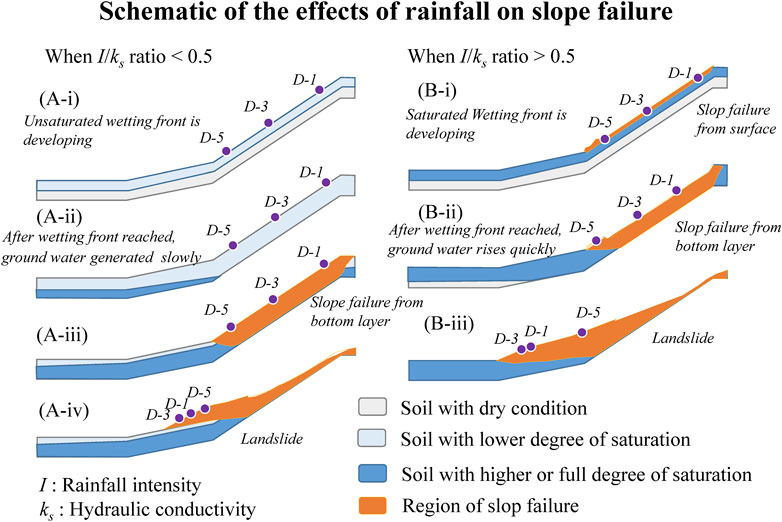
FIGURE 9. Schematic of the effects of rainfall on slope failure.

When the $I/k_s>0.5$, a wetting front developed with a high degree of saturation, which cause not only a decrease in the suction, but also an increase in the pore water pressure near the ground surface. Because the rainfall generated an increase in the pore water pressure from the ground surface, it resulted a shallow slope failure, as shown in Figure 9B-i. Hence, the surfaces of D-3 and D-1 began to move at this point. The depth of the slope failure increased corresponding to the growth of the wetting front, as shown in Figure 9A-ii. Until the wetting front reached the bottom soil layer, the slope with the 30° incline began to move entirely, as shown in Figure 9B-iii. According to the simulation shown in Figure 7C, the run-out distance increased with increases in the $I/k_s$ ratio. This implied that high intensity rainfall can easily induce a long run-out landslide.

Based on the parametric study, it was inferred that the rainfall intensity index plays an important role in distinguishing the slope failure pattern. In the case of the lab-scale rainfall-induced slope failure, the critical $I/k_s$ ratio was 0.5. At $I/k_s<0.5$, the slope failure was triggered by rising ground water, and the mechanism was similar to that of the rainfall-induced deep-seated landslide. At $I/k_s>0.5$, the slope failure was triggered by infiltration water, and the mechanism was close to that for a classic shallow landslide. This finding is important information that can be applied in the design of rainfall-induced landslide warning systems.

Conclusion

In this study, a numerical model using the material point method was applied to investigate the dynamic soil behavior of a rainfall-induced landslide. The proposed numerical model was implemented based on a set of pseudo-3-phase 1-point MPM formulations and overcame the limitations related to rainfall boundary conditions encountered in previous studies, so the effect of rainfall on the dynamic behavior of unsaturated soil could be investigated more comprehensively. A 1-D infiltration problem and a lab-scale rainfall-induced slope failure were performed to validate and benchmark the MPM code. Then, the proposed model was used to evaluate the effect of rainfall on the changes in pore water and slope failure. The following conclusions were drawn:

1) According to the effect of rainfall on changes in the pore water pressure, an important finding was that abnormally rising pore water pressure can be induced by high-intensity rainfall. The ratio of rainfall intensity and hydraulic conductivity ($I/k_s$) was introduced in this study. When the rainfall intensity was small, for example, $I/k_s=0.1$, the speed at which the pore water pressure rose was close to the hydraulic conductivity. However, when the rainfall intensity became strong, i.e., the $I/k_s$ ratio equaled 0.5, the speed at which the pore water pressure rose became over 10 times faster than the hydraulic conductivity. Because the changes in the pore water pressure change significantly influenced the stability of the slope, understanding changes in abnormal pore water pressure was deemed to be important. In this study, the $I/k_s$ ratio was considered to be a warning index to estimate a rainfall-induced abnormal rise in pore water pressure.

2) Based on the effects of rainfall on the slope failure, another important finding was that the types of slope failure were related to the magnitude of the rainfall intensity. In the case of lab-scale rainfall-induced slope failure, the types of slope failure could be distinguished by a critical value $I/k_s=0.5$, where when $I/k_s>0.5$, the numerical results showed that the wetting front developed with a higher degree of saturation and did not reduce the suction but increased the pore water pressure in the nearby ground surface. Hence, the slope failure began from the surface of the soil, and the mechanism was similar to that of a classic shallow landslide. When $I/k_s\le 0.5$, the wetting front developed with a lower degree of saturation, it only reduced the suction, and the slope remained in a stable state due to the contribution of friction force. Until the wetting front reached the bottom soil layer, pore water pressure was generated, which resulted in slope failure. The mechanism was similar to what occurs in a typical deep-seated landslide. This finding indicated that the $I/k_s$ ratio can be a warning index by which to estimate the failure types of rainfall-induced landslides.

In reality, the characteristics of landslide behavior are not only affected by the hydrological conditions but also are related to geological conditions and topography. With different constitutive models, the dynamic behavior of soil can be investigated and lead to different understandings of this phenomenon. Therefore, the proposed model should be modified with different constitutive models, so it will have more potential applications.

Data Availability Statement

The raw data supporting the conclusion of this article will be made available by the authors, without undue reservation.

Author Contributions

Conceptualization, W-LL and C-LS; methodology, W-LL and MM; formal analysis, W-LL and MM; W-LL wrote the manuscript, and all authors contributed to improving the paper.

Funding

This work was supported by the National Cheng Kung University (project of NCKU 90 and Beyond, HUA110-3-3-090).

Conflict of Interest

The authors declare that the research was conducted in the absence of any commercial or financial relationships that could be construed as a potential conflict of interest.

Publisher’s Note

All claims expressed in this article are solely those of the authors and do not necessarily represent those of their affiliated organizations, or those of the publisher, the editors and the reviewers. Any product that may be evaluated in this article, or claim that may be made by its manufacturer, is not guaranteed or endorsed by the publisher.

Supplementary Material

The Supplementary Material for this article can be found online at: https://www.frontiersin.org/articles/10.3389/feart.2021.764393/full#supplementary-material

References

Al-Kafaji, I. K. A. (2013). Formulation of a Dynamic Material point Method (MPM) for Geomechanical Problems. PhD Thesis. Stuttgart, Germany: Universität Stuttgart.
Bandara, S., Ferrari, A., and Laloui, L. (2016). Modelling Landslides in Unsaturated Slopes Subjected to Rainfall Infiltration Using Material point Method. Int. J. Numer. Anal. Meth. Geomech. 40 (9), 1358–1380. doi:10.1002/nag.2499
Bandara, S., and Soga, K. (2015). Coupling of Soil Deformation and Pore Fluid Flow Using Material point Method. Comput. geotechnics 63, 199–214. doi:10.1016/j.compgeo.2014.09.009
Calvello, M., Cascini, L., and Sorbino, G. (2008). A Numerical Procedure for Predicting Rainfall-Induced Movements of Active Landslides along Pre-existing Slip Surfaces. Int. J. Numer. Anal. Meth. Geomech. 32 (4), 327–351. doi:10.1002/nag.624
Cascini, L., Calvello, M., and Grimaldi, G. M. (2014). Displacement Trends of Slow-Moving Landslides: Classification and Forecasting. J. Mt. Sci. 11 (3), 592–606. doi:10.1007/s11629-013-2961-5
Cascini, L., Calvello, M., and Grimaldi, G. M. (2010). Groundwater Modeling for the Analysis of Active Slow-Moving Landslides. J. Geotech. Geoenviron. Eng. 136 (9), 1220–1230. doi:10.1061/(asce)gt.1943-5606.0000323
Ceccato, F., Girardi, V., Yerro, A., and Simonini, P. (2019). Evaluation of Dynamic Explicit MPM Formulations for Unsaturated Soils.
Ceccato, F., Yerro, A., Girardi, V., and Simonini, P. (2020). Two-phase Dynamic MPM Formulation for Unsaturated Soil. Comput. Geotechnics 129, 103876.
Cuomo, S., Ghasemi, P., Martinelli, M., and Calvello, M. (2019). Simulation of Liquefaction and Retrogressive Slope Failure in Loose Coarse-Grained Material. Int. J. Geomech. 19 (10), 04019116. doi:10.1061/(asce)gm.1943-5622.0001500
Cuomo, S. (2020). Modelling of Flowslides and Debris Avalanches in Natural and Engineered Slopes: a Review. Geoenviron Disasters 7 (1), 1–25. doi:10.1186/s40677-019-0133-9
Galavi, V. (2010). Groundwater Flow, Fully Coupled Flow Deformation and Undrained Analyses in PLAXIS 2D and 3D. Delft, Netherlands: Plaxis Report.
Ghasemi, P., Cuomo, S., Di Perna, A., Martinelli, M., and Calvello, M. (2019). MPM-analysis of Landslide Propagation Observed in Flume Test. Proc. Of II International Conference on the Material Point Method for Modelling Soil–Water–Structure Interaction. 8–10 January 2019. UK: University of Cambridge.
Jassim, I., Stolle, D., and Vermeer, P. (2013). Two-phase Dynamic Analysis by Material point Method. Int. J. Numer. Anal. Meth. Geomech. 37 (15), 2502–2522. doi:10.1002/nag.2146
Lee, W. L., Martinelli, M., and Shieh, C. L. (2019a). in Numerical Analysis of the Shiaolin Landslide Using Material Point Method. The 7th International Symposium on Geotechnical Safety and Risk (Taiwan, 638–643. https://10.3850/978-981-11-2725-0 IS7-2-cd.
Lee, W. L., Shieh, C. L., and Martinelli, M. (2019b). “Modelling Rainfall-Induced Landslides with the Material point Method: the Fei Tsui Road Case,” in Proceedings of the XVII European Conference on Soil Mechanics and Geotechnical Engineering. Iceland https://10.32075/17ECSMGE-2019-0346.
Lei, X., He, S., Chen, X., Wong, H., Wu, L., and Liu, E. (2020). A Generalized Interpolation Material point Method for Modelling Coupled Seepage-Erosion-Deformation Process within Unsaturated Soils. Adv. Water Resour. 141, 103578. doi:10.1016/j.advwatres.2020.103578
Leroueil, S. (2001). Natural Slopes and Cuts: Movement and Failure Mechanisms. Géotechnique 51 (3), 197–243. doi:10.1680/geot.51.3.197.39365
Leroueil, S., and Picarelli, L. (2012). Geotechnical Engineering State of the Art and Practice Keynote Lectures from GeoCongress 2012, 122–156. doi:10.1061/9780784412138.0006
Liu, X., Wang, Y., and Li, D.-Q. (2020). Numerical Simulation of the 1995 Rainfall-Induced Fei Tsui Road Landslide in Hong Kong: New Insights from Hydro-Mechanically Coupled Material point Method. Landslides 17 (12), 2755–2775. doi:10.1007/s10346-020-01442-2Assessment of Slope Stability
Liu, X., and Wang, Y. (2021). Probabilistic Simulation of Entire Process of Rainfall-Induced Landslides Using Random Finite Element and Material point Methods with Hydro-Mechanical Coupling. Comput. Geotechnics 132, 103989. doi:10.1016/j.compgeo.2020.103989
Martinelli, M., Lee, W.-L., Shieh, C.-L., and Cuomo, S. (2020). “Rainfall Boundary Condition in a Multiphase Material Point Method,” in Workshop on World Landslide Forum (Cham: Springer), 303–309. doi:10.1007/978-3-030-60706-7_29
Moriwaki, H., Inokuchi, T., Hattanji, T., Sassa, K., Ochiai, H., and Wang, G. (2004). Failure Processes in a Full-Scale Landslide experiment Using a Rainfall Simulator. Landslides 1 (4), 277–288. doi:10.1007/s10346-004-0034-0
Mualem, Y. (1976). A New Model for Predicting the Hydraulic Conductivity of Unsaturated Porous Media. Water Resour. Res. 12 (3), 513–522. doi:10.1029/WR012i003p00513
Nguyen, T. S., Yang, K. H., Ho, C. C., and Huang, F. C. (2021). Postfailure Characterization of Shallow Landslides Using the Material Point Method. London, United Kingdom: Geofluids.
Picarelli, L., Urciuoli, G., and Russo, C. (2004). Effect of Groundwater Regime on the Behaviour of Clayey Slopes. Can. Geotech. J. 41 (3), 467–484. doi:10.1139/t04-009
Siemens, G. A. (2018). Thirty-Ninth Canadian Geotechnical Colloquium: Unsaturated Soil Mechanics - Bridging the gap between Research and Practice. Can. Geotech. J. 55 (7), 909–927. doi:10.1139/cgj-2016-0709
Soga, K., Alonso, E., Yerro, A., Kumar, K., and Bandara, S. (2016). Trends in Large-Deformation Analysis of Landslide Mass Movements with Particular Emphasis on the Material point Method. Géotechnique 66 (3), 248–273. doi:10.1680/jgeot.15.lm.005
Sulsky, D., Zhou, S. J., and Schreyer, H. L. (1995). Application of a Particle-In-Cell Method to Solid Mechanics. Comp. Phys. Commun. 87 (1-2), 236–252. doi:10.1016/0010-4655(94)00170-7
Wang, B., Vardon, P. J., and Hicks, M. A. (2018). Rainfall-induced Slope Collapse with Coupled Material point Method. Eng. Geology. 239, 1–12. doi:10.1016/j.enggeo.2018.02.007
Yang, K.-H., Nguyen, T. S., Rahardjo, H., and Lin, D.-G. (2021). Deformation Characteristics of Unstable Shallow Slopes Triggered by Rainfall Infiltration. Bull. Eng. Geol. Environ. 80 (1), 317–344. doi:10.1007/s10064-020-01942-4
Yerro, A., Alonso, E. E., and Pinyol, N. M. (2015). The Material point Method for Unsaturated Soils. Géotechnique 65 (3), 201–217. doi:10.1680/geot.14.p.163
Yuan, W. H., Liu, K., Zhang, W., Dai, B., and Wang, Y. (2020). Dynamic Modeling of Large Deformation Slope Failure Using Smoothed Particle Finite Element Method. Landslides, 1–13. doi:10.1007/s10346-020-01375-w
Zhang, X., Chen, Z., and Liu, Y. (2016). The Material point Method: A Continuum-Based Particle Method for Extreme Loading Cases. Academic Press.
Keywords: landslide, rainfall boundary, infiltration, unsaturated soil, material point method
Citation: Lee W-L, Martinelli M and Shieh C-L (2021) An Investigation of Rainfall-Induced Landslides From the Pre-Failure Stage to the Post-Failure Stage Using the Material Point Method. Front. Earth Sci. 9:764393. doi: 10.3389/feart.2021.764393
Received: 25 August 2021; Accepted: 20 October 2021;
Published: 11 November 2021.
Edited by:
Rou-Fei Chen, Chinese Culture University, TaiwanReviewed by:
Joern Lauterjung, Helmholtz Centre Potsdam, GermanyQi Yao, China Earthquake Administration, China
Copyright © 2021 Lee, Martinelli and Shieh. This is an open-access article distributed under the terms of the Creative Commons Attribution License (CC BY). The use, distribution or reproduction in other forums is permitted, provided the original author(s) and the copyright owner(s) are credited and that the original publication in this journal is cited, in accordance with accepted academic practice. No use, distribution or reproduction is permitted which does not comply with these terms.
*Correspondence: Wei-Lin Lee, glaciallife@gmail.com; Mario Martinelli, mario.martinelli@deltares.nl