Emotion recognition from MIDI musical file using Enhanced Residual Gated Recurrent Unit architecture
 V. Bhuvana Kumar
  M. Kathiravan*
- Computer Science and Engineering, Hindustan Institute of Technology and Science, Chennai, India
The complex synthesis of emotions seen in music is meticulously composed using a wide range of aural components. Given the expanding soundscape and abundance of online music resources, creating a music recommendation system is significant. The area of music file emotion recognition is particularly fascinating. The RGRU (Enhanced Residual Gated Recurrent Unit), a complex architecture, is used in our study to look at MIDI (Musical Instrument and Digital Interface) compositions for detecting emotions. This involves extracting diverse features from the MIDI dataset, encompassing harmony, rhythm, dynamics, and statistical attributes. These extracted features subsequently serve as input to our emotion recognition model for emotion detection. We use an improved RGRU version to identify emotions and the Adaptive Red Fox Algorithm (ARFA) to optimize the RGRU hyperparameters. Our suggested model offers a sophisticated classification framework that effectively divides emotional content into four separate quadrants: positive-high, positive-low, negative-high, and negative-low. The Python programming environment is used to implement our suggested approach. We use the EMOPIA dataset to compare its performance to the traditional approach and assess its effectiveness experimentally. The trial results show better performance compared to traditional methods, with higher accuracy, recall, F-measure, and precision.
1 Introduction
The essence of music is deeply intertwined with emotion, as the emotional landscape of a musical piece can shift dramatically with variations in intensity, speed, and length. According to numerous studies (Juslin and Timmers, 2010; Ferreira and Whitehead, 2021), the close connection between musical structures and emotions has received a lot of attention in recent research, particularly in the fields of affective music composition and music emotion analysis. These investigations underscore the necessity of understanding how music's structural components influence emotional expression, a critical aspect for machines to effectively communicate and interact with human emotions (Koh and Dubnov, 2021). A song's mood can elicit a wide range of emotional responses from the listener (Krumhansl, 2002), with musical conventions like scale modes, dissonance, melody motion, and rhythm consistency playing a crucial role. The belief that the fundamental structure of music is the key to eliciting emotion has increased interest in music emotion recognition (MER) research (Chen et al., 2015; Panda et al., 2018). However, this field still faces numerous challenges and unresolved issues, particularly in the identification of emotions in audio music signals. A significant hurdle in MER is the subjective nature of emotional interpretation, as individuals may experience varying emotions when listening to the same piece of music. Another challenge lies in the need for standardized, high-quality audio emotion databases. Most musical notation software supports the MIDI format, which is common in symbolic music (Hosken, 2014; Li et al., 2018) and encapsulates the messages needed to create music with electronic instruments (Good, 2001; Renz, 2002; Nienhuys and Nieuwenhuizen, 2003). Recognizing emotions in MIDI musical files is crucial for enhancing the emotional impact of music, personalizing musical experiences, enabling music therapy, and advancing our understanding of music's emotional components (Luck et al., 2008; Nanayakkara et al., 2013). However, variations in emotion recognition can occur due to the dependency on the structure and properties of the MIDI file (Bresin and Friberg, 2000; Modran et al., 2023). MIDI files mostly show technical things like tempo and musical notation. They might not have the expressive range that performance dynamics, tone, and nuance can show. Additionally, the availability and quality of labeled emotional MIDI datasets may be limited (Shou et al., 2013). To address these challenges, this study introduces several contributions. We aim to recognize and extract statistical, harmonic, rhythmic, and dynamic elements from MIDI files. We use these features to improve a recognition model that is based on a better residual gated recurrent unit architecture. This model includes an adaptive algorithm, 'Neurons', for optimizing hyper-parameters like learning rate and GRU count. The proposed paradigm categorizes emotions into four quadrants: positive-high, positive-low, negative-high, and negative-low. It was implemented on the Python platform and evaluated using the EMOPIA dataset. The effectiveness of this approach is assessed using metrics such as accuracy, F-measure, precision, and recall.
2 Related works
The work at Panda et al. (2018) suggested adding different audio elements that are emotionally significant to fix the problems with current technology and get around their limitations. The researchers analyzed established frameworks and categorized their often-used audio elements into eight distinct musical groupings. A public dataset of 900 audio samples with subjective comments organized according to Russell's emotion quadrants was generated to assess their research efforts. Twenty cycles of 10-fold cross-validation were used to test the audio features that were already there (baseline) and the new features that were suggested for the novel. The F1-score was a noticeable 9% higher, or 76.4% higher, than the F1-score that was obtained using the proposed features along with the same number of baseline-only characteristics. The methodology has limitations in properly detecting alterations in emotional states. The paper Bhatti et al. (2016) advocated the utilization of brain signals as a means to discern human emotions in reaction to audio music tracks. The methodology utilized the readily accessible Narosky E.E.G. equipment to capture electroencephalogram (EEG) waves. In a controlled environment, individuals were instructed to engage in passive listening to audio recordings of music, with each genre lasting for 1 min. The main objectives of this study were to ascertain the age cohorts that exhibited greater receptivity to music and to assess the influence of different musical genres on human emotions. To accurately identify human emotions, the classifier included characteristics derived from three distinct domains: time, frequency, and wavelet. These features were retrieved from recorded EEG data. The study's findings unequivocally demonstrated that utilizing a multi-layer perceptron (MLP) model, incorporating a fusion of brain signal characteristics yielded remarkably high levels of accuracy in discerning human emotional states in response to audio-music stimuli. The article Hsu et al. (2017) introduced a computerized system that utilizes electrocardiogram (ECG) data to detect and classify human emotions. Firstly, the authors employ a musical induction technique to elicit the genuine emotional states of individuals and collect their ECG signals in a non-controlled laboratory setting. Subsequently, an algorithm was developed to enable automated detection of emotions by analyzing ECG signals, specifically targeting the emotional responses evoked in individuals through music perception. Using time-, frequency-, and non-linear methods to extract physiological ECG features allowed for the identification of emotion-relevant components and their correlation with emotional states. After that, a sequential forward floating selection-kernel-based class separability-based (SFFS-KBCS-based) feature selection algorithm is created to effectively find important ECG features connected to emotions and reduce the size of the chosen features. Furthermore, generalized discriminant analysis (GDA) is employed in this process. The research work Ghatas et al. (2022) introduced a method for automating piano difficulty estimation in symbolic music using deep neural networks. The researchers employ a computational model to replicate a piano recital based on a symbolic music MIDI file. Furthermore, the components of the piano roll were disassembled. Ultimately, a model was trained to utilize components assigned to difficulty labels. Our models were evaluated using both full-track and partial-track difficulty classification problems. Numerous deep convolutional neural networks have been both theorized and empirically examined. Combined with manually crafted features, the proposed hybrid deep model demonstrated exceptional performance, achieving a state-of-the-art F1 score of 76.26%. This achievement represents a significant improvement, with a relative F1 score gain of over 10% compared to previous studies. In their publication, Hung et al. (2021) introduced a novel public dataset called EMOPIA, which consists of a medium-scale collection of pop piano recordings accompanied by emotion descriptors. The given dataset includes a variety of types of data, such as MIDI transcriptions of compositions that only use piano, as well as emotional annotations at the clip level that are organized into four separate groups. The authors were provided with prototypes of models for categorizing musical emotions at the clip level and generating symbolic music based on emotions. These models were trained on the dataset and employed state-of-the-art techniques for their respective tasks. The findings indicated that the transformer-based model demonstrated a limited ability to generate music that elicited a predetermined emotional response. The researchers accurately categorized emotions in both four quadrant and valence-wise classifications. The work Ma et al. (2022) proposes a music creation model that incorporates emotional aspects and structural elements to make music. For making music, the suggested method used a conditional auto-regressive generative Gated Recurrent Unit (GRU) model. The authors collaborate to collectively optimize a perceptual loss and a cross-entropy loss throughout the training procedure. This optimization aims to enhance the emotional expression of the generated MIDI samples, closely resembling the original samples' emotional qualities. The results of both subjective and objective tests show that this model can create emotionally moving musical pieces that are very close to the structures that were given. Nevertheless, the system must build a comprehensive framework for evaluating the emotional impact of music. In the study Abboud and Tekli (2020), we introduced MUSEC, an innovative algorithmic framework designed for autonomous music sentiment-based expression and composition. The system identified six primary human emotions expressed in MIDI musical files: anger, fear, joy, love, sadness, and surprise. Subsequently, it generated novel polyphonic (pseudo) thematic compositions that properly conveyed the emotions above. The study's primary objective was to create a music composer grounded in sentimentality. The effectiveness of MUSEC was assessed in terms of feature parsing, sentiment expression, and music composition time. The technique has shown promise across various domains, such as music information retrieval, music composition, aided music therapy, and emotional intelligence. The research Malik et al. (2017) suggested a way to use layered convolution and recurrent neural networks to continuously predict emotions in the V-A space, which is only two dimensions. After setting up a single convolutional neural network (CNN) layer, the researchers used two separate types of recurrent neural networks (RNNs). These had each been trained in a different way to deal with arousal and valence. The methodology was evaluated using the “Media Eval 2015 Emotion in Music” dataset. To test how well the proposed Convolutional Recurrent Neural Network (CRNN) worked, sequences of different lengths were used. The results indicated that shorter durations exhibited superior performance compared to longer durations. The CRNN model shows that it can get information similar to baseline features by only using Mel-band features. Log Mel-band energy characteristics are suggested as a substitute for the baseline features.
3 Proposed methodology
In this study, the methodology for detecting emotions from MIDI musical files begins with extracting features from the dataset, which is crucial for the model's analysis, as shown in Figure 1. These features are fed into a new recognition model called an augmented residual gated recurrent unit. This model is made to accurately detect emotions. A key part of this process is optimizing the GRU's hyper-parameters using the adaptive Red Fox algorithm, enhancing the model's efficiency. The methodology culminates in classifying emotions into four quadrants: positive-high, positive-low, negative-high, and negative-low, allowing for a detailed understanding of the emotional spectrum in the music. This approach ensures precision in interpreting the emotional content of MIDI files, significantly contributing to emotion recognition in music. Enhanced RGRU MIDI musical file Emotion class PH: Positive-high PL: Positive-low NH: Negative-high NL: Negative-low Negative-low Feature extraction Hyperparameters Adaptive Red Fox algorithm.
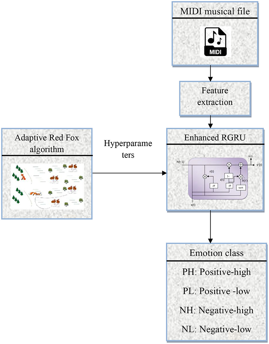
Figure 1. Emotion classification workflow for MIDI files.
3.1 Symbolic musical representation
Symbolic musical representation, similar to language modeling, involves converting MIDI files into discrete sequences of notes, mirroring musical events in a format akin to vocabulary (YGhatas et al., 2022). Tools like PrettyMIDI are used to extract specific details, such as each note's pitch, velocity, and duration. These details are then shown visually in Figure 2 using a set of pitch, duration, and hold elements. This is done through one-hot encoding, which turns complicated musical data into a format that is easy to understand. This method not only captures basic note elements but also encompasses key musical structures like melody, harmony, rhythm, and timbre, which are essential for understanding the emotional impact of music (Coutinho and Cangelosi, 2011).
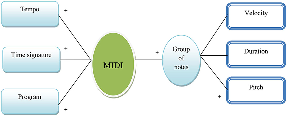
Figure 2. Components of MIDI data structure.
3.1.1 MIDI standard
The Musical Instrument Digital Interface (MIDI) is a symbolic music format that stands apart by recording musical performances using high-level music features, diverging from traditional audio formats that rely on low-level sound features. In MIDI, the focus is on abstractions like musical keys and chord progressions. A MIDI file typically consists of multiple tracks, each capable of independently playing a different instrument, providing a rich, layered musical experience (Sethares et al., 2005). Central to the MIDI format is the concept of the “tick,” which serves as the fundamental time unit. This unit is crucial in regulating all aspects of timing in a MIDI file, from the phases of notes to the intervals between them, ensuring a precise and accurate representation of musical timing.
3.2 Music feature extraction
Initially, the MIDI dataset's characteristics are extracted. There are rhythmic characteristics, dynamic characteristics, and statistical aspects.
3.2.1 Harmony features
Musical tones may be utilized to observe harmonics. The spectrogram of monophonic music reveals the harmonics with great clarity (Pickens and Crawford, 2002). In polyphony, where so many instruments and vocalists are used simultaneously, it is challenging to detect harmonics. A method for calculating harmonic distributions is the solution to this conundrum.
Here, Mh → the maximum number of harmonics to be considered. The most prevalent incidence of the phenomenon
f → Key frequency
S → The source signal's short-time Fourier transform (STFT).
The min function is applied to the equation so that only the powerful fundamentals and harmonics produce a significant HS value. After calculating the average of each frequency using (1), the standard deviation of each frequency was calculated.
3.2.2 Rhythmic features
Rhythm is a fundamental aspect of music, encompassing key rhythmic characteristics like tempo and cadence, which are essential in defining a musical piece's character. At the heart of musical cadence lies the beat, serving as the primary rhythm indicator. Tempo, a critical component of rhythm, is conventionally measured in beats per minute (BPM). This metric sets the overall rhythmic framework, dictating the speed and flow of the music (Fernández-Sotos et al., 2016). In practice, several techniques are employed to gauge the rate and consistency of these rhythmic pulses. To accurately determine the regularity and pace of the tempo, two main metrics are used: the overall tempo, which is quantified in pulses per minute, and the standard deviation of the intervals between beats. These measures together provide a comprehensive understanding of the tempo's stability and variation, thereby offering insights into the rhythmic structure that underpins the musical composition.
3.2.3 Dynamic features
Dynamics in music are deciphered by examining the pitch salience of every note in relation to others in the composition. Each note's intensity and its variation are determined by comparing it with the mean and standard deviation of all notes. Consequently, note intensities are classified as high (vigorous), medium, or low (smooth). Dynamic attributes, including RMS Energy, Low Energy Rate, Instantaneous Level, Frequency and Phase, Loudness, Timbral Width, Volume, Sound Balance, Note Intensity Statistics, and Note Intensity Distribution, encapsulate the essence of dynamic levels like forte and piano. Further nuances in dynamics are captured by metrics such as Transition Ratios, Crescendo, and Decrescendo (Panda et al., 2020).
3.3 Enhanced Residual Gated Recurrent Unit architecture
The advanced RGRU, a refined version of the GRU, is depicted in Figure 3, providing a detailed visual representation of its neural architecture. In this study, the recognition model for emotion detection in MIDI files employs an RGRU, into which extracted features are fed. The RGRU is designed to overcome the limitations of traditional GRU models, such as slow convergence and inadequate learning efficacy, particularly in handling complex time series data. Its innovative structure uses feedback from the reset gate to modify the update gate, enhancing the functionality and reducing redundant state information. This modification not only speeds up convergence but also significantly improves the model's learning capacity.
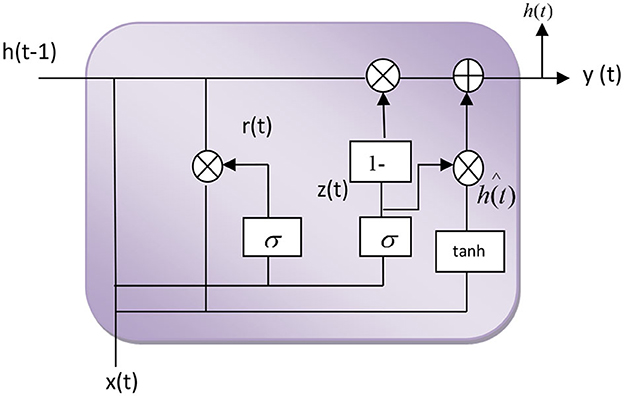
Figure 3. The structure of enhanced RGRU's neurons.
Assuming that the input sequence is (x1, x2,…, xt), followed by an update of the gate at t and a reset of the gate, the formula for calculating the standard, enhanced RGRU unit output is as follows:
The sigma “σ” typically represents the standard deviation, a measure of the amount of variation or dispersion in a set of values. While “V” represents the MIDI volume or velocity “V0” denotes the initial value of a variable represented by “V”.
The formula's symbols ztrt have the same significance as standard GRU—the neurons. According to Figure 3, the enhanced RGRU neuron differs from the GRU neuron in that it is multiplied by the previous time at the update gate to conceal the state weight, allowing the reset gate to rescreen the current input data. In other words, the output of the reset gate is used to modify the update gate to optimize the neuron structure and Equation (3), the enhanced RGRU. The neuron structure of the neural network is more logical than that of the GRU; the concealed state at each instant can be made more transparent, and gradient attenuation is moderately reduced. As a consequence, the RGRU was upgraded. The model's learning efficacy and prediction accuracy have improved, and it can maintain a greater dependence on distance information. The deep-enhanced RGRU neural network comprises input, output, and hidden layers. Neurons make up the concealed layers of the RGRU. Refining the GRU model's learning mechanism enhances the recursive transmission of information between neurons and the capacity to retain information.
3.3.1 Adaptive Red Fox algorithm
The ARFA is integrated to fine-tune the RGRU's hyperparameters, drawing inspiration from the hunting behavior of red foxes. This behavior, characterized by searching for prey in snow, is the foundation of the FOX algorithm (Cervený et al., 2011; Mohammed and Rashid, 2023). However, the red fox algorithm tends to converge prematurely, often getting stuck in local optima. To counter this, the Levy Flight method is incorporated, introducing diversity among search agents. This addition helps in avoiding local minima, thus enhancing the overall search efficiency and effectiveness of the algorithm. Consequently, combining the Levy Flight mechanism with the Red Fox algorithm enhances the optimization effectiveness. Figure 4 illustrates the hunting behavior of the red fox.
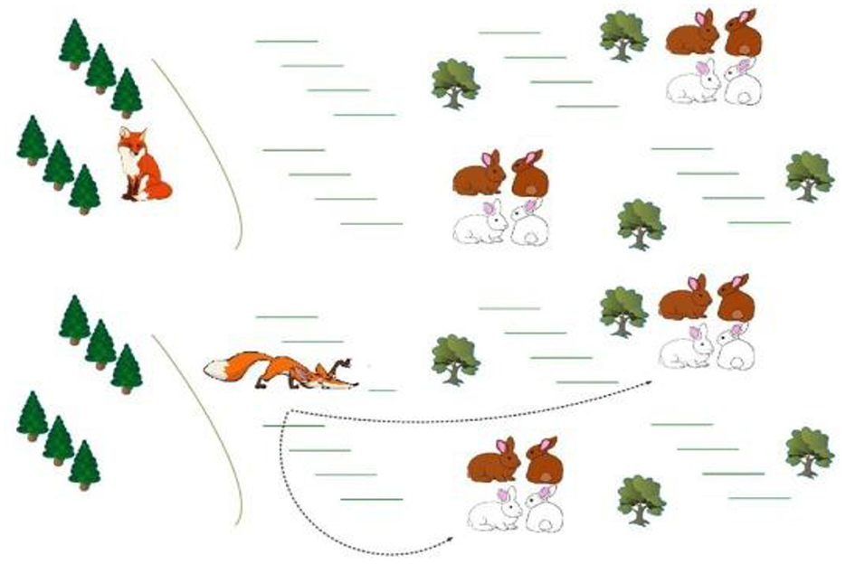
Figure 4. Fox and Rabbits interaction simulation.
The procedural steps are as follows:
• In the snow on the ground obstructing the prey's vision, the red fox resorts to random hunting.
• The red fox relies on ultrasonography emitted by the prey to locate it, followed by a period of approach.
• By listening to the prey's sounds and analyzing time intervals, the red fox determines the distance between itself and the prey.
• The establishing the prey's distance, the red fox calculates the required jump, proceeding with random walking based on the shortest distance and optimal position.
The steps involved in Adaptive Red Fox Algorithm are explained as follows:
(i) Initialization
The population, known as the Y matrix, is initially initialized by FOX. Red foxes' positions are represented by a Y. Here, hyperparameters such as GRU. Neurons (Gn) and the learning rate (l) should be considered solutions in this study.
(ii) Fitness function
Then, standard benchmark functions are used to assess the fitness of each search agent after each cycle. In order to find the best fitness () and matching optimal location, we compare the fitness values of individual search agents, represented by rows in an X matrix, to the fitness values of all other agents. The fitness of the previous rowFiti through the course of iterations is used. Fitness function (Fitn) can be calculated by using:
Accuracy, TP- true positive, FP- false positive, TN- true negative and FN- false negative. These values are crucial for calculating various performance metrics.
The formula (8) is used to measure the overall correctness of the model. Similarly, the following metrics are also successfully calculated:
Precision: TP/(TP + FP). This indicates the proportion of positive identifications that were actually correct.
Recall (Sensitivity): TP/(TP + FN). This shows the proportion of actual positives that were correctly identified.
F-Measure (F1 Score): 2 * (Precision * Recall)/(Precision + Recall). This is the harmonic mean of precision and recall, providing a balance between the two.
(iii) Update the solution
Exploitation Phase: This exploitation stage's random variable value is [0, 1]. Thus, the red fox's updated location must be determined while the random number is more significant than 0.18. Calculate the fox's distance from its prey (dpiter), sound's travel distance (dsiter), and jumping value (jiter) to update its location. To compute the distance between the sound and the red fox (dsiter), use the formula:
Sound travels Senv at 343 meters per second in the atmospheretstiter, a random value between 0 and 1. The iteration (iter) parameter ranges from 1 to 500. The distance between the fox (dsiter) and prey is calculated by halving (dpiter) and is given by:
The red fox must move after estimating the distance between it and the prey to jump and seize it. The fox must calculate its jump height (jiter) by:
To equal the average sound travel time, 9.81 equals gravitational acceleration squared by the jump's up-and-down steps. If a random value between 0 and 1 is more critical than 0.18, the red fox's new location is found using Equations (14) and (15). Only one is executed per iteration due to the p condition. The revised position is calculated using equation (14) if it is more significant than 0.18. Equations determine the current position if the result is less than 0.18 (15). The variable ranges from [0, 0.18] to [0.19, 1]. These values are based on a red fox's leaps toward or away from the northeast. The red fox's new location is estimated using the equation below.
The value 0.18 was empirically determined to optimize the algorithm's performance, ensuring a balanced and effective search mechanism in the exploitation phase of the Adaptive Red Fox Algorithm. This threshold value is a key factor in the algorithm's ability to accurately and efficiently mimic the strategic hunting pattern of a red fox.
Exploration Phase: During this phase, a fox randomly pursues the best location so far to regulate its random walking. At this stage, the fox could not jump because it had to wander throughout the search area in pursuit of prey. The search is controlled to ensure that the fox wanders randomly to the ideal location using the minimal time variable minTv and the variable z. Following that, the average time t is determined by dividing Tt by 2. Equations (15) and (16) calculate the minTvz and variables. Equation (14) can be used to calculate the time transitionTt.
Use this method to make sure that the fox checks out the food in a random way. The best answer (Yiter) found significantly affects the exploration phase. The fox's approach to exploring the search space Y(it+1)as it looks for a new place to go is shown in Equation (17).
Levy flight: When Levy Flight (LF) is implemented, it optimizes the diversity of search agents, ensuring that the algorithm will effectively explore a position while achieving the lowest local avoidance possible.
Here, it represents mean entry-wise multiplication, is the ith Fox location at iteration, μ is a uniformly distributed random value, and finally denotes a random number falling between [0, 1].sign[rand−1/2] I only had three values, which were 1, 0, and 1. The Levy Flight produced the following random walk distributions.
Levy flight step lengths sl are as follows:
λ is constructed using the formula for λ = 1+β where the identical normal stochastic distributions with
Incorporating the Levy Flight mechanism into the search process introduces a diversity that allows for a more comprehensive exploration of the solution space, thereby improving the effectiveness of the overall optimization process.
(iv) Termination
The above phases are continued until the optimal solution or optimal weights of RGRU are reached. Otherwise, the algorithm will be terminated. Levy Flight will significantly improve the Red Fox algorithm's search capabilities and protect against local minima.
4 Result and discussion
The implementation of our proposed emotion recognition technique was carried out using Python. In this study, we focused on checking how computationally efficient different processing steps are in the Python environment, such as training and classification. For the assessment, we utilized the Classical Music MIDI dataset, featuring works from nineteen renowned composers, sourced from Piano MIDI. This offered a wide variety of classical piano MIDI files, some of which had audio versions to accompany the playing of the scores. In our methodology, 20% of the dataset was dedicated to evaluating the generation model, with the remaining 80% used for training. Section 4.2 details the performance analysis of the model.
4.1 Dataset analysis
The EMOPIA dataset that was used in this study gives a lot of information about each sample, such as related data, segmentation annotations, and Jensen-Shannon divergence for different emotion quadrant pairs. To facilitate the use of MusPy, MIDI data has been incorporated into the library. However, due to copyright constraints, audio files are not directly released; instead, YouTube links are provided for access. The availability of these songs is subject to the copyright laws of the respective countries and the decisions of the rights holders regarding their availability on the platform.
The study delves into an array of musical elements that are instrumental in shaping the emotions experienced by listeners. The study aims to find out how the different MIDI features are distributed across the four emotional quadrants in order to figure out how these musical features are related to emotions in EMOPIA. The study picks out and shows the most distinguishing features of the different aspects that were looked at, giving us information about the most important parts of music that affect how we feel.
The frequency and intensity of note occurrences serve to measure music arousal, as depicted in Figure 5. This is gauged using three metrics: note length, note density, and note velocity. Note density is the number of notes per beat, and note length is the average duration of a note within a beat. Note velocity, obtained from MIDI data, reflects the strength of each note. These metrics are essential in understanding the music's rhythmic and dynamic properties, corresponding to the emotional states.
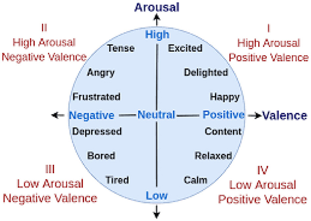
Figure 5. Distribution of different emotions on arousal-valence space.
4.2 Performance analysis
The developed model in this study aims to categorize emotions into four distinct quadrants: positive-high, positive-low, negative-high, and negative-low. To evaluate its effectiveness, the model employs the EMOPIA dataset. Key performance indicators used for assessment include accuracy, precision, recall, and F-score. A big part of this study is comparing how well the new RGRU model works with other models like GRU, LSTM, and CNN. The next part will go into more detail about this comparison by looking at how well the proposed approach works compared to these well-known classification models using a number of different performance metrics.
4.2.1 Performance analysis of positive high quadrant
Figure 6 presents the confusion matrices for the positive high quadrant, summarizing the predictive accuracy of different classification models. The proposed RGRU model correctly identified 157 instances as Positive High and another 120 instances as not belonging to this class. This shows how accurate the model is, with only two false positives and one false negative. This indicates strong model performance with high true positive and true negative rates, coupled with very few misclassifications.
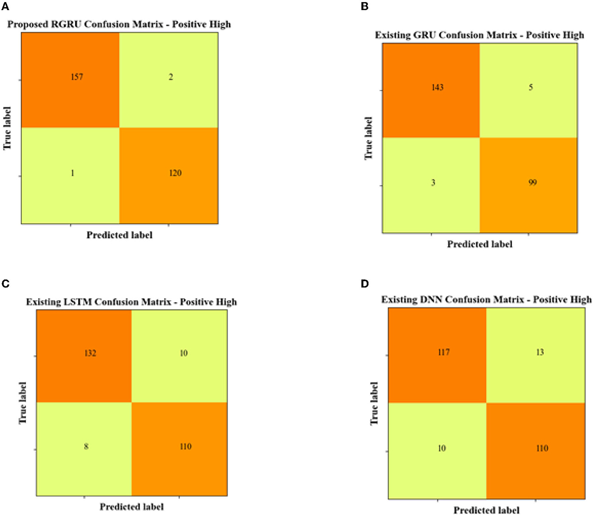
Figure 6. Confusion matrix for positive high. (A) Proposed RGRU. (B) Existing GRU. (C) Existing LSTM. (D) Existing DNN.
In contrast, the existing GRU model demonstrates slightly diminished accuracy, with 143 true positives and 99 true negatives. It also recorded a higher number of false classifications, with five false positives and three false negatives. The LSTM model follows a similar trend but with more pronounced inaccuracies, tallying 132 true positives and 110 true negatives, alongside 10 false positives and eight false negatives. With only 117 true positives and 110 true negatives, the DNN model is the most different from the proposed RGRU model. It also has the highest error rate, with 13 false positives and 10 false negatives. Overall, the RGRU model does better than the others because it consistently makes more correct predictions and fewer mistakes. This suggests that it is the most reliable model for identifying the Positive High quadrant in this study.
Figure 7 shows the ROC and AUC graphs for the positive high quadrant. The ROC curve shows the trade-off between sensitivity (or TPR) and specificity (1-FPR). Classifiers that give curves closer to the top-left corner indicate better performance. The AUC provides an aggregate measure of performance across all possible classification thresholds. It is the area under the ROC curve, with a value between 0 and 1. A model with perfect predictive accuracy would have an AUC of 1, meaning it has a good measure of separability. A model with no discriminative power has an AUC of 0.5, meaning it does as well as random chance.
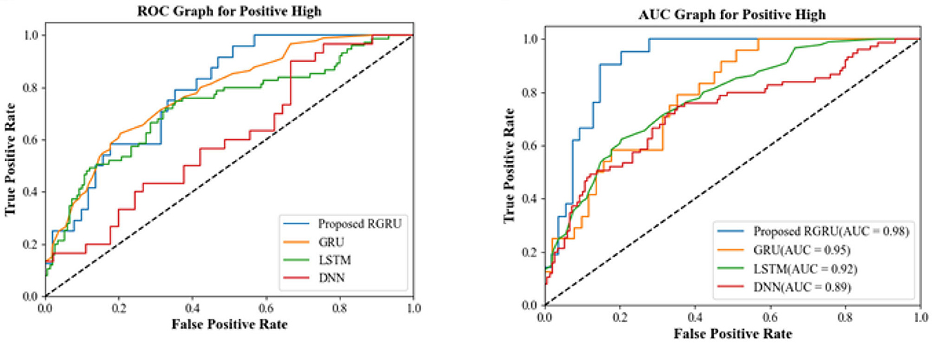
Figure 7. R.O.C. and A.U.C. graph for positive high.
From the research work, for the positive high quadrant, the proposed RGRU has the highest AUC, indicating it outperforms the other models in distinguishing between the positive high class and the not-positive high class. Existing GRU performs better than LSTM and DNN, but the proposed RGRU outperforms them both. The existing LSTM has a lower AUC than RGRU and GRU but is higher than DNN, suggesting moderate performance. Likewise, the existing DNN has the lowest AUC, indicating the least performance in comparison to the other models. The ROC and AUC graphs demonstrate that the proposed RGRU model has a superior ability to classify the positive high quadrant with more accuracy than the other models.
To see how well the suggested RGRU method works, we look at important performance indicators like accuracy, precision, recall, F-measure, and more, which can be seen in Figure 8 and Table 1. We check how well this method works with the Long Short-Term Memory (LSTM), Gated Recurrent Unit (GRU), and Deep Neural Network (DNN) classification methods. With a maximal accuracy of 98.92%, the RGRU technique significantly outperforms alternative models, including LSTM (5.75%), GRU (2.18%), and DNN (8.12%). When compared to the alternative methods, the RGRU strategy exhibits superior performance, as evidenced by its F-measure (99.05%), precision (98.74%), and recall (99.36%). The results obtained from the enhanced adaptive red fox algorithm (ARFA) are superior to those obtained from alternative methods, specifically when it comes to identifying positive high-phase emotions, as demonstrated by the table and graph depicted. This serves as a demonstration of how the proposed approach surpasses the present condition of affairs.
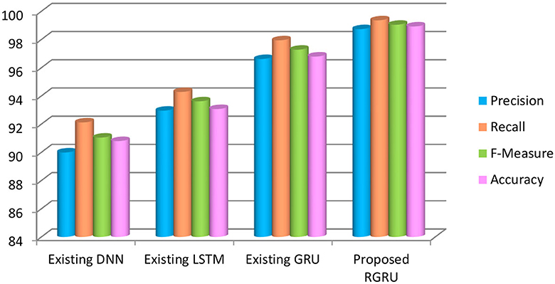
Figure 8. Precision, recall, F-measure and accuracy-based analysis of various models (positive high).
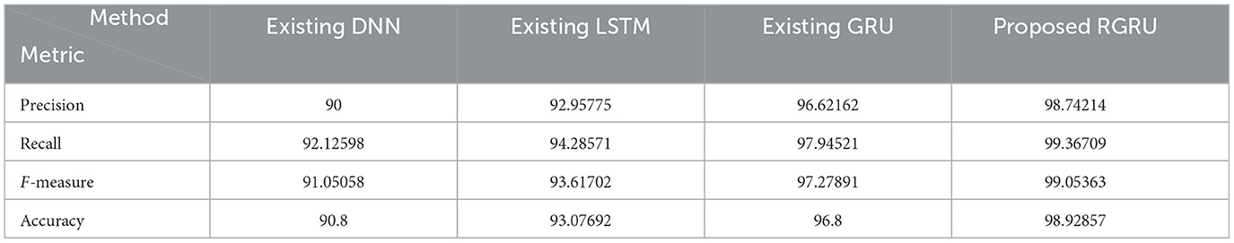
Table 1. The performance evaluation of various models (positive high).
4.2.2 Performance analysis of positive low quadrant
The confusion matrix data for the Positive Low quadrant show that the proposed RGRU model is the most accurate, with 130 true positives and 120 true negatives. This shows that it is very good at correctly classifying instances. With only two false positives and a single false negative, it demonstrates remarkable precision in detection. Comparatively, the existing GRU model identified 124 true positives and 119 true negatives but had slightly more misclassifications, with seven false positives and three false negatives. The LSTM model registered 120 true positives and 115 true negatives, with its accuracy further diminished by 10 false positives and 8 false negatives. The DNN model matched the LSTM in true positives but fell behind with only 110 true negatives, and it exhibited the highest error rates, having misclassified 13 false positives and 10 false negatives. Overall, the RGRU model's superior performance is evidenced by its higher correct classifications and minimal errors, affirming its effectiveness in the positive low quadrant compared to the GRU, LSTM, and DNN models.
Figure 9 shows the confusion matrix for the positive low quadrant, and Figure 10 shows the ROC and AUC graph for the positive low quadrant.
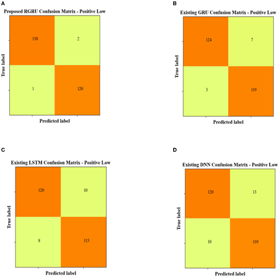
Figure 9. Confusion matrix for positive low. (A) Proposed RGRU. (B) Existing GRU. (C) Existing LSTM. (D) Existing DNN.
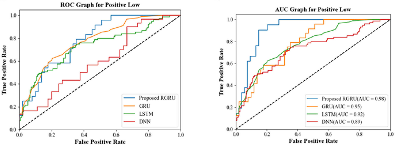
Figure 10. R.O.C. and A.U.C. graph for positive low.
The ROC and AUC graphs for the positive low quadrant provide insightful measures of model performance. The ROC graph illustrates the balance between sensitivity and specificity, with the proposed RGRU model's curve approaching the ideal top-left corner more closely than the others, signaling its superior performance in correctly identifying true positives while minimizing false positives. The curves of the existing GRU, LSTM, and DNN models don't show this optimal balance as clearly. They lie below that of the RGRU, which means they don't make the trade-off as well.
With an AUC of 0.98, the proposed RGRU model gets the highest score in the AUC graph, which shows how well it does across all possible classification thresholds. This shows that it is very good at telling the difference between classes. The existing models, on the other hand, have lower AUC values-−0.95 for GRU, 0.92 for LSTM, and 0.89 for DNN—which means they are less accurate at classifying things. Together, these AUC scores support what the confusion matrices and the ROC graph showed: the proposed RGRU model is better than the current GRU, LSTM, and DNN models at classifying the Positive Low quadrant with more accuracy and a better ability to tell the classes apart.
In Figure 11 and Table 2, the study assesses the effectiveness of the proposed RGRU method using metrics such as precision, recall, F-measure, and accuracy. This method is compared against three alternative classification methods: GRU, LSTM, and DNN. The results shown in Figure 11 show that the RGRU method is more accurate than GRU by 2.77%, LSTM by 5.93%, and DNN by 7.91%. This demonstrates that the proposed RGRU method achieves the highest accuracy among the compared methods. Furthermore, the proposed approach also records the highest precision at 98.48%, recall at 99.23%, and F-measure at 98.85%. The table unmistakably demonstrates that the RGRU, with the Adaptive Red Fox Algorithm (ARFA) enhancement, performs better than the other techniques, especially in the positive low phase of emotion recognition. This highlights the effectiveness of the RGRU method in outperforming competing approaches.
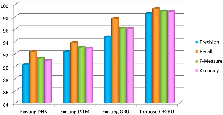
Figure 11. Precision, recall, F-measure and accuracy-based analysis of various models (positive low).
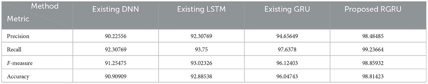
Table 2. The performance evaluation of various models (positive low).
4.2.3 Performance analysis of negative high quadrant
The proposed RGRU model stands out in the Negative High confusion matrix with 154 true positives, which correctly identify Negative High instances, and 120 true negatives, which correctly identify non-Negative High instances. It demonstrates a robust classification capability with only three false positives and an equal number of false negatives.
The current GRU model has a higher count of 187 true positives, but it is less accurate with eight false positives and five false negatives, which means that wrong classifications are more likely to happen. On the other hand, the LSTM model, with 162 true positives and 120 true negatives, also displays an increased rate of misclassification, as evidenced by 18 false positives and 10 false negatives, which underscores a potential compromise in model reliability.
The DNN model, despite having a commendable number of 130 true negatives, falls short in accuracy, with the lowest true positive count at 145 and the highest false positive count at 25, accompanied by 10 false negatives. This indicates a substantial reduction in its efficacy in the negative high quadrant compared to the RGRU model.
In essence, the RGRU model's performance in the negative high quadrant surpasses that of the GRU, LSTM, and DNN models, as reflected by its higher correct predictions and lower misclassifications, showcasing its effectiveness and reliability in emotion classification within this specific context.
Figure 12 shows the confusion matrix for the negative high quadrant, and Figure 13 shows the ROC and AUC graph for the negative high quadrant. The proposed RGRU model demonstrates superior proficiency, with its curve nearing the top-left corner, an indication of an excellent balance between sensitivity and specificity. In comparison, the curves representing the GRU, LSTM, and DNN models are positioned lower, signifying a less optimal trade-off and reduced effectiveness in distinguishing the negative high class.
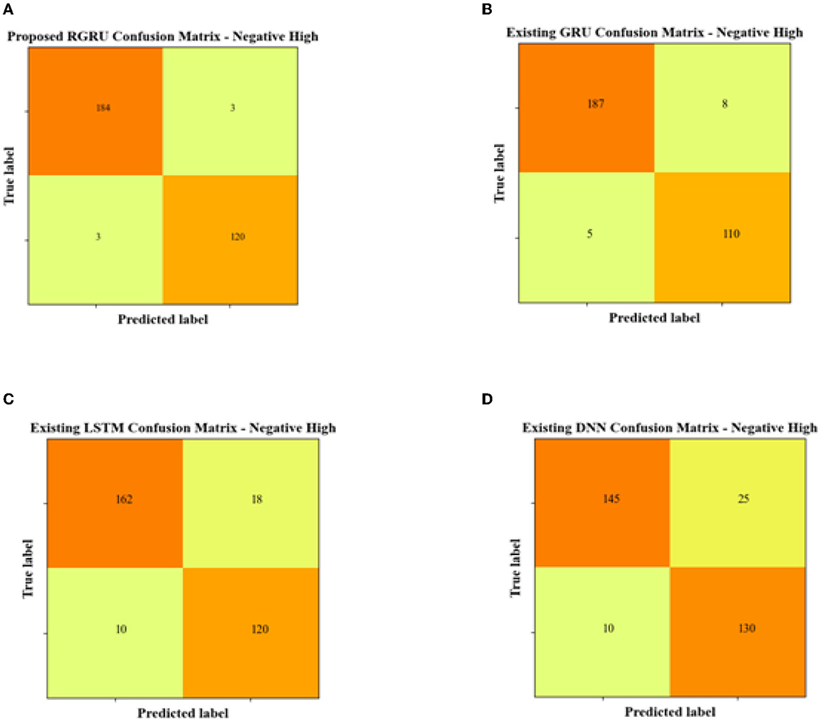
Figure 12. Confusion matrix for negative high. (A) Proposed RGRU. (B) Existing GRU. (C) Existing LSTM. (D) Existing DNN.
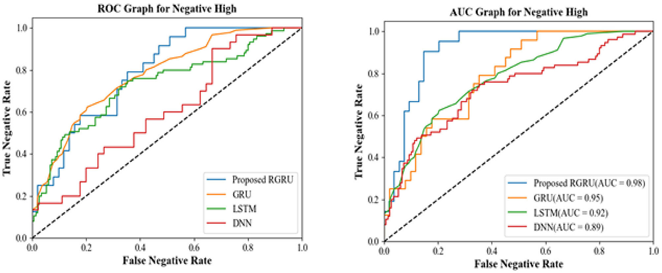
Figure 13. R.O.C. and A.U.C. graph for negative high.
AUC, measures a model's accuracy over a broad range of threshold values. The RGRU model's AUC value of 0.98 indicates that it has a significant ability to differentiate classes. The classification performance of the DNN model is 0.89, whilst the LSTM model shows a performance of 0.92. With an AUC of 0.95, however, the GRU model performs better than both.
To assess the effectiveness of the strategy depicted in Figure 14 and Table 3, accuracy, precision, recall, and the F-measure are used. Using these measures, we compare our proposed RGRU technique against three distinct classification strategies: GRU, LSTM, and DNN. Our technique has a maximum accuracy of 98.06%, outperforming GRU by 2.26%, LSTM by 7.1%, and DNN by 9.36%. Our technique's improved performance is also visible in other parameters, such as recall (98.24%), precision (96.39%), and F-measure (98.39%). Table 3 shows the results of the public inspection technique that we proposed. The results show that our strategy was effective throughout the negative high phase; the improved performance of the RGRU is attributed to the Adaptive Red Fox Algorithm (ARFA). This contrast highlights the enormous advances that our proposed methodology offers to the problem of emotion categorization.
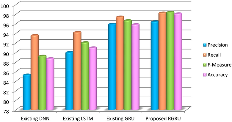
Figure 14. Precision, recall, F-measure and accuracy-based analysis of various models (negative high).
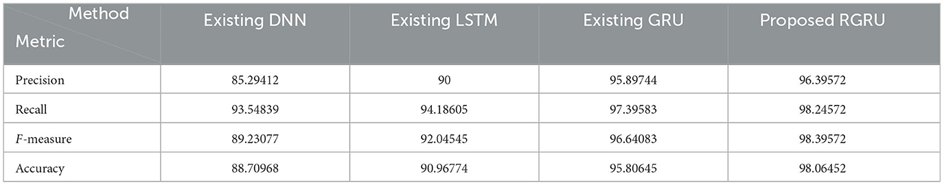
Table 3. The performance evaluation of various models (negative high).
4.2.4 Performance analysis of negative low quadrant
The proposed RGRU model's confusion matrix does a great job in the negative low quadrant, with a high number of true positives (169) and true negatives (90). This means that the classification is correct, with only a few cases being wrongly labeled (false positives at 3) or missed (false negatives also at 3). This suggests a precise model for identifying negative and low emotions. The current GRU model, on the other hand, has a slightly lower level of accuracy than the RGRU model, with 162 true positives and 90 true negatives. This is because it has more false positives (8) and false negatives (5).
Increased misclassifications, with 136 true positives and 100 true negatives, but also a noticeable rise in both false positives (19) and false negatives (10), highlight the LSTM model's further decreased performance and suggest that it is less reliable for accurate classification of negative low emotions. The DNN model presents the lowest performance in the group, with the lowest count of true positives (121) and the highest count of false negatives (15), coupled with a considerable number of false positives (19). The DNN model's confusion matrix clearly illustrates its challenges in accurately classifying negative emotions, with considerable room for improvement in its predictive capabilities.
Figure 15 shows the confusion matrix for the negative low quadrant, and Figure 16 shows the ROC and AUC graph for the negative low quadrant. For the negative low quadrant, the ROC and AUC graphs provide insightful measures of each model's performance.
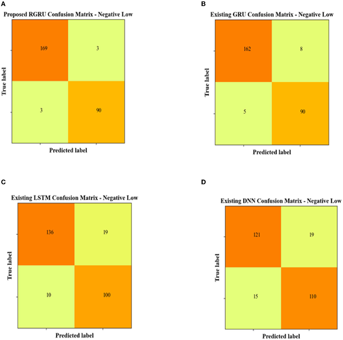
Figure 15. Confusion matrix for negative low. (A) Proposed RGRU. (B) Existing GRU. (C) Existing LSTM. (D) Existing DNN.
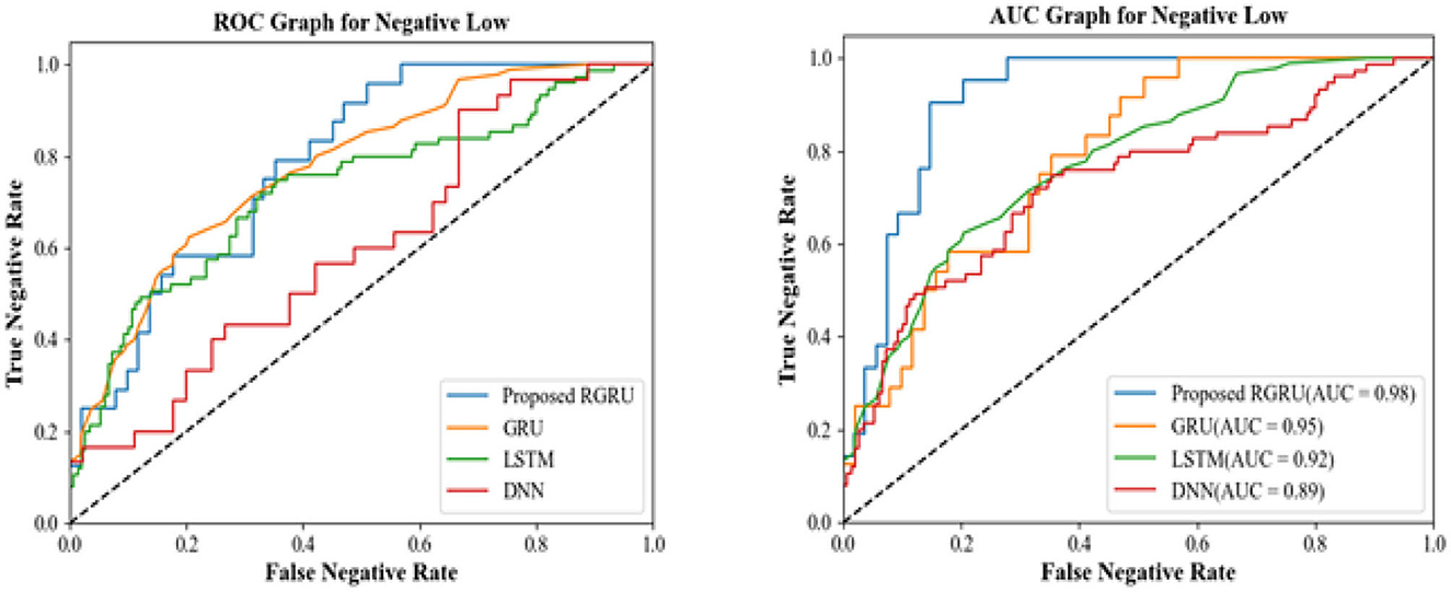
Figure 16. R.O.C. and A.U.C. graph for negative low.
The ROC graph for the proposed RGRU model showcases an optimal balance between the true negative rate and the false negative rate, with its curve being the closest to the ideal top-left corner. This shows a better ability to tell the difference between Negative Low and other classes without labeling instances that aren't Negative Low as Negative Low by accident. The ROC curves for the GRU, LSTM, and DNN models are farther from the ideal point, which means that their balance between sensitivity and specificity is not as good. These models have a lower true negative rate for any given false negative rate, signifying a reduced ability to accurately classify negative emotions.
The AUC value for the RGRU model stands at 0.98, the highest among the models, demonstrating its outstanding overall classification performance. This high AUC value means that the RGRU model has a good chance of correctly identifying any given case as either negative or not, for all thresholds. The GRU, LSTM, and DNN models have lower AUC scores (0.95, 0.92, and 0.89, respectively), which means they can't tell the difference between negative low and non-negative low classes as well-across all thresholds. The RGRU model, which performs better at classifying negative low emotions than the GRU, LSTM, and DNN models, supports the confusion matrix results according to the ROC and AUC graphs. The RGRU model is better because it is closer to the ideal points on the graphs, has higher true negative rates, and has a higher AUC value. These factors show that it is better at telling the difference between negative and low emotions and overall performance.
Figure 17 and Table 4 show how well the suggested RGRU-based method works by checking its precision, recall, F-measure, and accuracy. This evaluation involves a comparative analysis with other classification algorithms, namely GRU, LSTM, and DNN. Our suggested method performs much better than the others, with a maximum accuracy of 97.73%, which is 2.64% higher than GRU, 8.68% higher than LSTM, and 10.57% higher than DNN. This makes it the most accurate method we looked at.
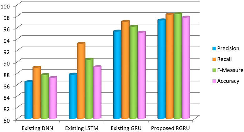
Figure 17. Precision, recall, F-measure and accuracy-based analysis of various models (negative low).
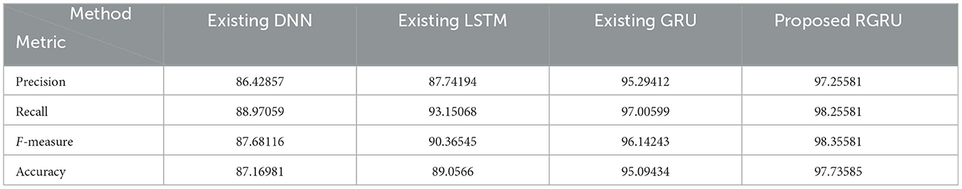
Table 4. The performance evaluation of various models (negative low).
Furthermore, the suggested method performs exceptionally well in important measures, with an F-measure of 98.35%, a precision rate of 97.25%, and a recall rate of 98.25%. As detailed in Table 4, these statistics prominently showcase the method's superior performance compared to other techniques. Particularly noteworthy is the method's performance in the negative low phase, as highlighted in the results section. We think this better performance is because the Adaptive Red Fox Algorithm (ARFA) was used to improve the RGRU. This makes it much better at classifying emotions. I made the right choice by using both RGRU and ARFA in my research. Together, they help reach the goals of the study, specifically by making emotion recognition from MIDI files more accurate and reliable.
The combination of these advanced methods aligns perfectly with the research objectives of accurately identifying and classifying emotions in MIDI musical files. The RGRU's architecture is well-suited for the sequential and temporal nature of music data, while ARFA ensures that the model operates at its highest potential. They work well together to show that these methods are complete and accurate for detecting emotions in MIDI files, proving that they are good for the research goals. The MIDI dataset used in this study appears reliable, as MIDI files accurately encode detailed musical information crucial for emotion recognition. The study's results were checked using statistical methods like F-score, accuracy, precision, and recall to measure the model's performance in a quantitative way. We found these results to be even more important by comparing them to results from well-known models like GRU, LSTM, and DNN. This showed that the new model was better at recognizing emotions from MIDI files.
5 Conclusion
This study has introduced a novel approach to discerning the emotional nuances embedded within each MIDI composition, utilizing the enhanced RGRU architecture for hyperparameter optimization through ARFA. We used the EMOPIA dataset and performance metrics like precision, F-measure, recall, and accuracy to do a full evaluation of our proposed method to see how well it worked. In the comparative analysis against the existence prediction models, including GRU, LSTM, and DNN, the proposed approach consistently outperformed them in all four quadrants: positive-high (98.92%), positive-low (98.91%), negative-high (98.06%), and negative-low (97.73%). These results underscore our innovative methodologies' superior predictive accuracy and overall efficacy.
While emotion recognition in music is a recognized field, its specific application to MIDI compositions is relatively less explored. This research adds originality by focusing on analyzing emotions in MIDI data, which can have unique challenges compared to other audio formats.
The research relies on the EMOPIA dataset for evaluation. If this dataset has biases or limitations regarding diversity and representation of musical emotions, it can impact the generalizability of the findings. The study demonstrates the effectiveness of the proposed approach, but it may not necessarily generalize well to different music genres, styles, or cultural contexts. It's important to acknowledge the scope of its applicability. Emotion recognition in music is inherently subjective. The model's interpretation of emotions might not fully capture the individual listener's experience, potentially leading to discrepancies between the model's classifications and human perception.
Future research should aim to diversify datasets for broader genre coverage, develop algorithms for nuanced emotion detection, ensure hardware scalability, and refine emotion classification methods. These steps will enhance the model's accuracy and applicability in diverse musical and cultural settings, ensuring its effectiveness in real-world scenarios.
Data availability statement
The original contributions presented in the study are included in the article/supplementary material, further inquiries can be directed to the corresponding author.
Author contributions
VK: Conceptualization, Data curation, Formal analysis, Methodology, Software, Visualization, Writing – original draft, Writing – review & editing. MK: Conceptualization, Data curation, Investigation, Methodology, Project administration, Resources, Supervision, Validation, Visualization, Writing – review & editing.
Funding
The author(s) declare that no financial support was received for the research, authorship, and/or publication of this article.
Conflict of interest
The authors declare that the research was conducted in the absence of any commercial or financial relationships that could be construed as a potential conflict of interest.
Publisher's note
All claims expressed in this article are solely those of the authors and do not necessarily represent those of their affiliated organizations, or those of the publisher, the editors and the reviewers. Any product that may be evaluated in this article, or claim that may be made by its manufacturer, is not guaranteed or endorsed by the publisher.
References
Abboud, R., and Tekli, J. (2020). Integrating nonparametric fuzzy classification with an evolutionary-developmental framework to perform music sentiment-based analysis and composition. Soft Comp. 24, 9875–9925. doi: 10.1007/s00500-019-04503-4
Bhatti, A. M., Majid, M., Anwar, S. M., and Khan, B. (2016). Human emotion recognition and analysis in response to audio music using brain signals. Comput. Human Behav. 65, 267–275. doi: 10.1016/j.chb.2016.08.029
Bresin, R., and Friberg, A. (2000). The emotional colouring of computer-controlled music performances. Comp. Music J. 24, 44–63. doi: 10.1162/014892600559515
Cervený, J., Begall, S., Koubek, P., Nováková, P., and Burda, H. (2011). Directional preference may enhance hunting accuracy in foraging foxes. Biol. Lett. 7, 355–357. doi: 10.1098/rsbl.2010.1145
Chen, S. H., Lee, Y. S., Hsieh, W. C., and Wang, J. C. (2015). “Music emotion recognition using deep Gaussian process,” in 2015, the Asia-Pacific Signal and Information Processing Association Annual Summit and Conference (APSIPA) (Taiwan: IEEE), 495–498.
Coutinho, E., and Cangelosi, A. (2011). Musical emotions: predicting second-by-second subjective feelings of emotion from low-level psychoacoustic features and physiological measurements. Emotion 11, 921. doi: 10.1037/a0024700
Fernández-Sotos, A., Fernández-Caballero, A., and Latorre, J. M. (2016). Influence of tempo and rhythmic unit in musical emotion regulation. Front. Comput. Neurosci. 10, 80. doi: 10.3389/fncom.2016.00080
Ferreira, L. N., and Whitehead, J. (2021). Learning to generate music with sentiment. arXiv [06125].
Ghatas, Y., Fayek, M., and Hadhoud, M. (2022). A hybrid deep learning approach for musical difficulty estimation of piano symbolic music. Alexandria Eng. J. 61, 10183–10196. doi: 10.1016/j.aej.2022.03.060
Hsu, Y. L., Wang, J. S., Chiang, W. C., and Hung, C. H. (2017). Automatic ECG-based emotion recognition in music listening. IEEE Transact. Affect. Comp. 11, 85–99. doi: 10.1109/TAFFC.2017.2781732
Hung, H. T., Ching, J., Doh, S., Kim, N., Nam, J., and Yang, Y. H. (2021). EMOPIA: a multi-modal pop piano dataset for emotion recognition and emotion-based music generation. arXiv.
Juslin, P. N., and Timmers, R. (2010). “Expression and communication of emotion in music performance,” in Handbook of Music and Emotion: Theory, Research, Applications (Washington, DC: Oxford University Press), 453–489.
Koh, E., and Dubnov, S. (2021). “Comparison and analysis of deep audio embeddings for music emotion recognition,” AAAI Workshop on Affective Content Analysis. New York, NY: Cornell University.
Krumhansl, C. L. (2002). Music: a link between cognition and emotion. Curr. Dir. Psychol. Sci. 11, 45–50. doi: 10.1111/1467-8721.00165
Li, B., Liu, X., Dinesh, K., Duan, Z., and Sharma, G. (2018). Creating a multitrack classical music performance dataset for multi-modal music analysis: challenges, insights, and applications. IEEE Transact. Multimedia 21, 522–535. doi: 10.1109/TMM.2018.2856090
Luck, G., Toiviainen, P., Erkkilä, J., Lartillot, O., Riikkilä, K., Mäkelä, A., et al. (2008). Modelling the relationships between emotional responses to and the musical content of music therapy improvisations. Psychol. Music 36, 25–45. doi: 10.1177/0305735607079714
Ma, L., Zhong, W., Ma, X., Ye, L., and Zhang, Q. (2022). Learning to generate emotional music correlated with music structure features. Cogn. Comp. Syst. 4, 100–107. doi: 10.1049/ccs2.12037
Malik, M., Adavanne, S., Drossos, K., Virtanen, T., Ticha, D., and Jarina, R. (2017). Stacked convolutional and recurrent neural networks for music emotion recognition. arXiv. doi: 10.23919/EUSIPCO.2017.8081505
Modran, H. A., Chamunorwa, T., Ursuţiu, D., Samoilă, C., and Hedeşiu, H. (2023). Using deep learning to recognize therapeutic effects of music based on emotions. Sensors 3, 986. doi: 10.3390/s23020986
Mohammed, H., and Rashid, T. (2023). FOX: a FOX-inspired optimization algorithm. Appl. Intell. 53, 1030–1050. doi: 10.1007/s10489-022-03533-0
Nanayakkara, S. C., Wyse, L., Ong, S. H., and Taylor, E. A. (2013). Enhancing the musical experience for people who are deaf or hard of hearing using visual and haptic displays. Hum. Comp. Interact. 28, 115–160.
Nienhuys, H.-W., and Nieuwenhuizen, J. (2003). “LilyPond, a system for automated music engraving,” in Proceedings of the XIV Colloquium on Musical Informatics (XIV CIM 2003), Vol. 1 (Switzerland: Citeseer), 167–171.
Panda, R., Malheiro, R., and Paiva, R. P. (2018). Novel audio features for music emotion recognition. IEEE Transact. Affect. Comp. 11, 614–626. doi: 10.1109/TAFFC.2018.2820691
Panda, R., Malheiro, R. M., and Paiva, R. P. (2020). Audio features for music emotion recognition: a survey. IEEE Transact. Affect. Comp.
Pickens, J., and Crawford, T. (2002). “Harmonic models for polyphonic music retrieval,” in Proceedings of the Eleventh International Conference on Information and Knowledge Management (University of London), 430–437.
Renz, K. (2002). Algorithms and Data Structures for a Music Notation System Based on Guido Music Notation (Ph.D. thesis), Darmstadt: Technische Universita.
Sethares, W. A., Morris, R. D., and Sethares, J. C. (2005). Beat tracking of musical performances using low-level audio features. IEEE Transact. Speech Audio Process. 13, 275–285. doi: 10.1109/TSA.2004.841053
Shou, L., Mao, K., Luo, X., Chen, K., Chen, G., and Hu, T. (2013). “Competence-based song recommendation,” in Proceedings of the 36th International ACM SIGIR Conference on Research and Development in Information Retrieval (Zhejiang University, China), 423–432.
Keywords: emotion recognition, Musical Instrument Digital Interface, Enhanced Residual Gated Recurrent Unit, adaptive Red Fox algorithm, EMOPIA
Citation: Kumar VB and Kathiravan M (2023) Emotion recognition from MIDI musical file using Enhanced Residual Gated Recurrent Unit architecture. Front. Comput. Sci. 5:1305413. doi: 10.3389/fcomp.2023.1305413
Received: 01 October 2023; Accepted: 30 November 2023;
Published: 21 December 2023.
Edited by:
Mariacarla Martí-González, University of Valladolid, SpainReviewed by:
N. Bharathiraja, Chitkara University, IndiaJiri Pribil, Slovak Academy of Sciences, Slovakia
Copyright © 2023 Kumar and Kathiravan. This is an open-access article distributed under the terms of the Creative Commons Attribution License (CC BY). The use, distribution or reproduction in other forums is permitted, provided the original author(s) and the copyright owner(s) are credited and that the original publication in this journal is cited, in accordance with accepted academic practice. No use, distribution or reproduction is permitted which does not comply with these terms.
*Correspondence: M. Kathiravan, mkathiravan@hindustanuniv.ac.in