Manifold-driven decomposition for adversarial robustness
 Wenjia Zhang
 Yikai Zhang2
  Xiaoling Hu
 Mayank Goswami
 Chao Chen
 Dimitris Metaxas
- 1Department of Computer Science, Rutgers University, Piscataway, NJ, United States
- 2Morgan Stanley, New York, NY, United States
- 3Department of Computer Science, Stony Brook University, Stony Brook, NY, United States
- 4SRI International, Computer Vision Lab, Princeton, NJ, United States
- 5Department of Computer Science, Queens College of CUNY, New York, NY, United States
- 6Department of Biomedical Informatics, Stony Brook University, Stony Brook, NY, United States
The adversarial risk of a machine learning model has been widely studied. Most previous studies assume that the data lie in the whole ambient space. We propose to take a new angle and take the manifold assumption into consideration. Assuming data lie in a manifold, we investigate two new types of adversarial risk, the normal adversarial risk due to perturbation along normal direction and the in-manifold adversarial risk due to perturbation within the manifold. We prove that the classic adversarial risk can be bounded from both sides using the normal and in-manifold adversarial risks. We also show a surprisingly pessimistic case that the standard adversarial risk can be non-zero even when both normal and in-manifold adversarial risks are zero. We finalize the study with empirical studies supporting our theoretical results. Our results suggest the possibility of improving the robustness of a classifier without sacrificing model accuracy, by only focusing on the normal adversarial risk.
1 Introduction
Machine learning (ML) algorithms have achieved astounding success in multiple domains such as computer vision (Krizhevsky et al., 2012; He et al., 2016), natural language processing (Wu et al., 2016; Vaswani et al., 2017), and robotics (Levine and Abbeel, 2014; Nagabandi et al., 2018). These models perform well on massive datasets but are also vulnerable to small perturbations on the input examples. Adding a slight and visually unrecognizable perturbation to an input image can completely change the prediction of the model. Many studies have been published, focusing on such adversarial attacks (Szegedy et al., 2013; Carlini and Wagner, 2017; Madry et al., 2017). To improve the robustness of these models, various defense methods have been proposed (Madry et al., 2017; Shafahi et al., 2019; Zhang et al., 2019). These methods mostly focus on minimizing the adversarial risk, i.e., the risk of a classifier when an adversary is allowed to perturb any data with an oracle.
Despite the progress in improving the robustness of models, it has been observed that compared with a standard classifier, a robust classifier often has a lower accuracy on the original data. The accuracy of a model can be compromised when one optimizes its adversarial risk. This phenomenon is called the trade-off between robustness and accuracy. Su et al. (2018) observed this trade-off effect on a large number of commonly used model architectures. They concluded that there is a linear negative correlation between the logarithm of accuracy and adversarial risk. Tsipras et al. (2018) proved that adversarial risk is inevitable for any classifier with a non-zero error rate. Zhang et al. (2019) decomposed the adversarial risk into the summation of standard error and boundary error. The decomposition provides the opportunity to explicitly control the trade-off. They also proposed a regularizer to balance the trade-off by maximizing the boundary margin.
In this study, we investigate the adversarial risk and the robustness-accuracy trade-off through a new angle. We follow the classic manifold assumption, i.e., data are living in a low dimensional manifold embedded in the input space (Cayton, 2005; Niyogi et al., 2008; Narayanan and Mitter, 2010; Rifai et al., 2011). Based on this assumption, we analyze the adversarial risk with regard to adversarial perturbations within the manifold and normal to the manifold. By restricting to in-manifold and normal perturbations, we define the in-manifold adversarial risk and normal adversarial risk. Using these new risks, together with the standard risk, we prove an upper bound and a lower bound for the adversarial risk. We also show that the bound is tight by constructing a pessimistic case. We validate our theoretical results using synthetic and real-world datasets.
Our study sheds light on a new aspect of the robustness-accuracy trade-off. Through the decomposition into in-manifold and normal adversarial risks, we might find an extra margin to exploit without confronting the trade-off.
A preliminary version of this study, which mainly focuses on the theoretical results, was published in the study mentioned in the reference (Zhang et al., 2022). The major differences between this article and Zhang et al. (2022) include the adding of experimental validation on real-world datasets to verify our theoretical discoveries. To realize this validation process, we employ the Tangent-Normal Adversarial Regularization algorithm (TNAR) by Yu et al. (2019), which obtain the normal and in-manifold directions within real data. This strategic utilization of Tangent-Normal Adversarial Regularization algorithm not only strengthens the empirical foundation of our research but also indicates our commitment to bridging the gap between theoretical insights and practical applicability. By integrating this experimental result, we not only refines the theoretical framework but also provides an empirical verification, enhancing the overall credibility and relevance of our research findings.
1.1 Related works
Robustness-accuracy trade-off: It was believed that a classifier cannot be optimally accurate and robust at the same time. Different articles study the trade-off between robustness and accuracy (Su et al., 2018; Tsipras et al., 2018; Dohmatob, 2019; Zhang et al., 2019). One main question is whether the best trade-off actually exists. Tsipras et al. (2018) first recognized this trade-off phenomenon by empirical results and further proved that the trade-off exists under the infinite data limit. Dohmatob (2019) showed that a high accuracy model can inevitably be fooled by the adversarial attack. Zhang et al. (2019) gave examples showing that the Bayes optimal classifier may not be robust.
However, others have different views on this trade-off or even its existence. In contrast to the idea that the trade-off is unavoidable, according to these studies, the drop of accuracy is not due to the increase in robustness. Instead, it is due to a lack of effective optimization methods (Shaham et al., 2018; Awasthi et al., 2019; Rice et al., 2020) or better network architecture (Fawzi et al., 2018; Guo et al., 2020). Yang et al. (2020) showed the existence of both robust and accurate classifiers and argued that the trade-off is influenced by the training algorithm to optimize the model. They investigated distributionally separated dataset and claimed that the gap between robustness and accuracy arises from the lack of a training method that imposes local Lipschitzness on the classifier. Remarkably, in the study mentioned in the reference (Carmon et al., 2019; Gowal et al., 2020; Raghunathan et al., 2020), it was shown that with certain augmentation of the dataset, one may be able to obtain a model that is both accurate and robust.
Our theoretical results upperbound the adversarial risk using different manifold-derived risks plus the standard Bayes risk (which is essentially the accuracy). This quantitative relationship provides a pathway toward an optimal robustness-accuracy trade-off. In particular, our results suggest that, by adversarial training, the model against perturbations in the normal direction can improve robustness without sacrificing accuracy.
Manifold assumption: One important line of research focuses on the manifold assumption on the data distribution. This assumption suggests that observed data are distributed on a low dimensional manifold (Cayton, 2005; Narayanan and Mitter, 2010; Rifai et al., 2011), and there exists a mapping that embeds the low dimension manifold in some higher dimension space. Traditional manifold learning methods (Tenenbaum et al., 2000; Saul and Roweis, 2003) that try to recover the embedding by assuming the mapping preserves certain properties such as distances or local angles. Following this assumption, on the topic of robustness, Tanay and Griffin (2016) showed the existence of adversarial attack on the flat manifold with linear classification boundary. It was proved later (Gilmer et al., 2018) that in-manifold adversarial examples exist. They stated that high-dimension data are highly sensitive to l2 perturbations and pointed out that the nature of adversarial is the issue with potential decision boundary. Later, Stutz et al. (2019) showed that with the manifold assumption, regular robustness is correlated with in-manifold adversarial examples, and therefore, accuracy and robustness may not be contradictory goals. Further discussion (Xie et al., 2020) even suggested that adding adversarial examples to the training process can improve the accuracy of the model. Lin et al. (2020) used perturbation within a latent space to approximate in-manifold perturbation. Most existing studies only focused on in-manifold perturbations. To the best of our knowledge, we are the first to discuss normal perturbation and normal adversarial risk. We are also unaware of any theoretical results proving upper/lower bounds for adversarial risk in the manifold setting.
We also note a classic manifold reconstruction problem, i.e., reconstructing a d-dimensional manifold given a set of points sampled from the manifold. A large group of classical algorithms (Edelsbrunner and Shah, 1994; Dey and Goswami, 2006; Niyogi et al., 2008) are probably good, i.e., they give a guarantee of reproducing the manifold topology with a sufficiently large number of sample points.
Under data manifold assumption, Stutz et al. (2019) and Shamir et al. (2021) first reconstruct the data manifold using Generative Networks. Then, with the approximation of manifold, the authors explored different approaches for computing in-manifold attack examples under manifold assumption. Stutz et al. (2019) approximate the data manifold using VAE models and then directly perturbed the latent space without considering the perturbed distance in the original space, making it difficult to bound their on-manifold examples. On the other hand, Shamir et al. (2021) first perturbed the latent code to generate a set of basis in the tangential space, using these basis vectors to generate on-manifold directions and search for in-manifold attack examples. In the study by Lau et al. (2023), the author employs generative model-based methods to simultaneously perturb the input data in both the original space and the latent space. This dual perturbation process results in in-manifold perturbed data even on high-resolution datasets.
The Tangent-Normal Adversarial Regularization (TNAR) algorithm (Yu et al., 2019) distinguishes itself by finding tangential directions along the data manifold through power iteration and conjugate gradient algorithms. Subsequently, we perform a targeted search along these tangential directions to find valid Lp norm-based adversarial examples while ensuring effective perturbation bounds on the in-manifold examples.
2 Manifold-based risk decomposition
In this section, we state our main theoretical result (Theorem 1), which decomposes the adversarial risk into normal adversarial risk and in-manifold (or tangential) adversarial risk. We first define these quantities and set up basic notations. Next, we state the main theorem in Section 2.3. For the sake of simplicity, we describe our main theorem in the setting of binary labels, {−1, 1}. Informally, the main theorem states that under mild assumptions, (1) the adversarial risk can be upper-bounded by the sum of the standard risk, normal adversarial risk, in-manifold adversarial risk, and another small risk called nearby-normal-risk; (2) when the normal adversarial risk is zero, the adversarial risk can be upper-bounded by the standard risk and the in-manifold adversarial risk. Finally, we show in Theorem 2 that the bounds are tight by constructing pessimistic cases.
2.1 Data manifold
Let (ℝD, ||.||) denote the D dimensional Euclidean space with ℓ2-norm, and let p be the data distribution. For x ∈ ℝD, let Bϵ(x) be the open ball of radius ϵ in ℝD with center at x. For a set A ⊂ ℝD, define Bϵ(A) = {y:∃x ∈ A, d(x, y) < ϵ}.
Let be a d-dimensional compact smooth manifold embedded in ℝD. Thus, for any x ∈ M, there is a corresponding coordinate chart (U, g), where U ∋ x is an open set of and g is a homeomorphism from U to a subset of ℝd. Let and denote the tangent and normal spaces at x. Intuitively, the tangent space is the space of tangent directions or equivalence classes of curves in passing through x, with two curves considered equivalent if they are tangent at x. The normal space is the set of vectors in ℝD that are orthogonal to any vector in . Since is a smooth d-manifold, and are d and (D − d) dimensional vector spaces, respectively (see Figure 1 for an illustration). For detailed definitions, we refer the reader to the study mentioned in the reference (Bredon, 2013).
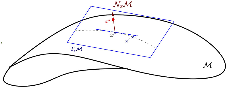
Figure 1. Tangent and normal spaces of a manifold. Here, x is the original data point on the data manifold . is the tangent space along the data manifold at point x. x′ is the in-manifold adversarial example on the data manifold . denotes the normal space perpendicular to . x* is an adversarial perturbation along .
We assume that the data and (binary) label pairs are drawn from , according to some unknown distribution p(x, y). Note that is unknown. A score function f(x) is a continuous function from ℝD to [0, 1]. We denote by 1A the indicator function of the event A that is 1 if A occurs and 0 if A does not occur and will use it to represent the 0-1 loss.
2.2 Robustness and risk
Given data from drawn according to data distribution p and a classifier f on ℝD, we define three types of risks. The first, adversarial risk, has been extensively studied in machine learning literature:
Definition 1 (Adversarial risk). Given ϵ > 0, define the adversarial risk of classifier f with budget ϵ to be
Notice that Bϵ(x) is the open ball around x in ℝD (the ambient space).
Next, we define risk that is concerned only with in-manifold perturbations. Previously, Gilmer et al. (2018) and Stutz et al. (2019) showed that there exist in-manifold adversarial examples and empirically demonstrated that in-manifold perturbations are a cause of the standard classification error. Therefore, in the following, we define the in-manifold perturbations and in-manifold adversarial risk.
Definition 2 (In-manifold Adversarial Risk). Given ϵ > 0, the in-manifold adversarial perturbation for classifier f with budget ϵ is the set
The in-manifold adversarial risk is
We remark that while the above perturbation is on the manifold, many manifold-based defense algorithms use generative models to estimate the homeomorphism (the manifold chart) z = g(x) for real-world data. Therefore, instead of in-manifold perturbation, one can also use an equivalent η-budget perturbation in the latent space. However, for our purposes, the in-manifold definition will be more convenient to use. Finally, we define the normal risk:
Definition 3 (Normal adversarial risk). Given ϵ > 0, the normal adversarial perturbation for classifier f with budget ϵ is be the set
Define the normal adversarial risk as
Notice that the normal adversarial risk is non-zero if there is an adversarial perturbation x′ ≠ x in the normal direction at x. Finally, we have the usual standard risk: Rstd(f): = 𝔼(x, y)~p𝟙(f(x)y ≤ 0).
2.3 Main result: decomposition of risk
In this section, we state our main result that decomposes the adversarial risk into its tangential and normal components. Our theorem will require a mild assumption on the decision boundary DB(f) of the classifier f, i.e., the set of points x where f(x) = 0.
Assumption [A]: For all x ∈ DB(f) and all neighborhoods U ∋ x containing x, there exist points x0 and x1 in U such that f(x0) < 0 and f(x1) > 0.
This assumption states that a point that is difficult to classify by f has points of both labels in any given neighborhood around it. In particular, this means that the decision boundary does not contain an open set. We remark that both Assumption A and the continuity requirement for the score function f are implicit in previous decomposition results such as Equation 1 in the study by Zhang et al. (2019). Without Assumption A, the “neighborhood” of the decision boundary in the study by Zhang et al. (2019) will not contain the decision boundary, and it is easy to give a counterexample to Equation 1 in the study by Zhang et al. (2019) if f is not continuous.
Our decomposition result will decompose the adversarial risk into the normal and tangential directions: however, as we will show, an “extra term” appears, which we define next:
Definition 4 (NNR Nearby-Normal-Risk). Fix ϵ > 0. Denote by A(x, y) the event that i.e., the normal adversarial risk of x is zero.
Denote by B(x, y) the event that
i.e., x has a point x′ near it such that x′ has non-zero normal adversarial risk.
Denote by C(x, y) the event , i.e., x has no adversarial perturbation in the manifold within distance 2ϵ.
The Nearby-Normal-Risk (denoted as NNR) of f with budget ϵ is defined to be
where ∧ denotes “and”.
We are now in a position to state our main result.
Theorem 1. [Risk Decomposition] Let be a smooth compact manifold in ℝD and let data be drawn from , according to some distribution p. There exists a Δ > 0 depending only on such that the following statements hold for any ϵ < Δ. For any score function f satisfying assumption A,
(I)
(II) If , then
Remark:
1. The first result decomposes the adversarial risk into the standard risk, the normal adversarial risk, the in-manifold adversarial risk, and an “extra term”—the Nearby-Normal-Risk. The NNR comes into play when a point x does not have normal adversarial risk, and the score function on all points nearby agrees with y(x), yet there is a point near x that has non-zero normal adversarial risk.
2. The second result states that if the normal adversarial risk is zero, the ϵ-adversarial risk is bounded by the sum of the standard risk and the 2ϵ in-manifold adversarial risk.
3. Our bound suggests that there may be “free lunch” in robustness-accuracy trade-off. There is an extra margin one can exploit without confronting the trade-off. Specifically, this corollary suggests that by solely minimizing the normal adversarial risk, we can govern the difference between adversarial risk and standard accuracy by focusing exclusively on in-manifold adversarial risk. This insight provides a pathway to navigating the trade-off under the condition of zero normal adversarial risk, wherein the key lies in minimizing the in-manifold risk. This strategic approach opens up ways for fine-tuning and optimizing the robustness-accuracy trade-off, shedding light on potential methods for achieving better performance on robust models.
One may wonder if a decomposition of the form is possible. We prove that this is not possible. The complete proof of Theorem 1 is technical and is provided in the Supplementary material. Here, we provide a sketch of the proof first.
2.3.1 Proof sketch of theorem 1
We first address the existence of the constant Δ that only depends on in the theorem statement. Define a tubular neighborhood of as a set containing such that any point has a unique projection π(z) onto such that . Thus, the normal line segments of length ϵ at any two points are disjoint.
By Theorem 11.4 in the study by Bredon (2013), we know that there exists Δ such that is a tubular neighborhood of . The Δ guaranteed by Theorem 11.4 is the Δ referred to our theorem, and the budget ϵ is constrained to be at most Δ.
For simplicity, we first sketch the proof of the case when y is deterministic (the setting of Corollary 1). Considering a pair (x, y) ~ p, x has an adversarial perturbation x′ within distance ϵ. We show that one of the four cases must occur:
• x′ = x (standard risk).
• x′ ≠ x, , and f(x)y > 0 (normal adversarial risk).
• Let x″ = π(x′) (the unique projection of x′ onto ), then d(x″, x) ≤ 2ϵ and either
* f(x″)y ≤ 0 and x have an 2ϵ in-manifold adversarial perturbation (in-manifold adversarial risk) or
* f(x″)f(x′) ≤ 0, which implies that x is within 2ϵ of a point that has non-zero normal adversarial risk (NNR: nearby-normal-risk).
The second of these sets is Znor(f, ϵ) in the setting of Corollary 1. One can observe that the four cases correspond to the four terms in Equation 2.
For the proof of Theorem 1, one has to observe that since y is not deterministic, the set Znor(f, ϵ) is random. One then has to average over all possible Znor(f, ϵ) and show that the average equals NNR.
For the second part of Theorem 1 and Corollary 1, we observed that if the normal adversarial risk is zero, in the last case, x″ has non-zero normal adversarial risk, with normal adversarial perturbation x′. Unless x″ is on the decision boundary, by continuity of f one can show that there exists an open set around x″ such that all points have non-zero normal adversarial risk. This contradicts the fact that the normal adversarial risk is zero, implying that case 4 happens only on a set of measure zero (recalling that by assumption A, the decision boundary does not contain any open set). This completes the proof sketch.
Theorem 2. [Tightness of decomposition result]
For any ϵ < 1/2, there exists a sequence of continuous score functions such that
(I) Rstd(f) = 0 for all n ≥ 1,
(II) for all n ≥ 1, and
(III) as n goes to infinity,
but Radv(f, ϵ) = 1 for all .
Thus, all three terms, except the NNR term, indicate zero, but the adversarial risk (the left side of Equation 2) indicates one.
Here, we provide a sketch of the proof of Theorem 2. Then, we give the complete proof in the Supplementary material.
2.3.2 Proof of theorem 2
Let and fix ϵ < 1/2 and n ≥ 1. We will think of data as lying in the manifold and ℝ2 as the ambient space. The true distribution is simply η(x) = 1 for all , hence y ≡ 1 (all labels on are 1).
Let and . Note that (n + 1)ℓ1 + nℓ2 = 1. Consider the following partition of , where Ai (0 ≤ i ≤ n) is of length ℓ1 and Bi (1 ≤ i ≤ n) is an interval of length ℓ2. The interval A0, B1, A1, ⋯ , Bn, An appears in this order from left to right.
For ease of presentation, we will consider {0, 1} binary labels and build score functions fn, taking values in [0, 1] that satisfy the conditions of the Theorem.
For an x ∈ Ai for some 0 ≤ i ≤ n, define gn(x) = 1. For x ∈ Bi for some 1 ≤ i ≤ n, define gn(x) = ϵ/2. Observe that ϵ/2 < 1/4.
We now define the decision boundary of fn as the set of points in ℝ2 on the “graph” of gn and −gn. That is,
(see Figure 2 for a picture of the upper decision boundary).
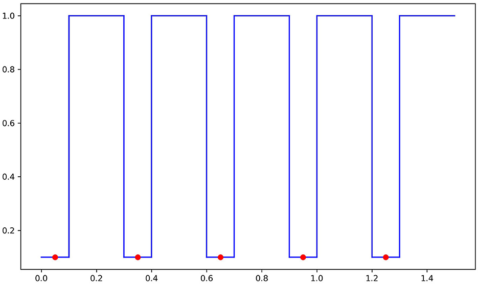
Figure 2. Lower bound illustration.
Now, let fn be any continuous function with decision boundary DB(fn) as above. That is, is such that fn(x, t) > 1/2 if |t| < gn(x), fn(x, t) < 1/2 if |t| > gn(x) and fn(x, y) = 1/2 if |t| = gn(x).
In-manifold adversarial risk is zero: Observe that since η(x) = 1 on [0, 1], the in-manifold adversarial risk of fn is zero, since fn(x, 0) > 1/2, and so sign(2fn−1) equals 1, which is the same as the label y at x. This means that there are no in-manifold adversarial perturbations, no matter the budget. Thus, for all n ≥ 1.
Normal adversarial risk goes to zero: Next, we consider the normal adversarial risk. If x ∈ Ai for some i, a point in the normal ball with budget ϵ is of the form (x, t) with |t| < ϵ < 1/2 but fn(x, t)>1/2 for such points and thus sign (2fn−1) = y(x). Thus, x ∈ Ai does not contribute to the normal adversarial risk. If x ∈ Bi for some i then fn(x, ϵ) < 1/2 while fn(x, 0) > 1/2, and hence such x contributes to the normal adversarial risk. Thus, , which goes to zero as n goes to infinity.
Adversarial risk goes to one: Now, we show that Radv(fn, ϵ) goes to one. In fact, we will show that as long as n is sufficiently large, the adversarial risk is 1. Consider n such that . Note that such an n exists simply because ℓ1 goes to zero as n goes to infinity and works.
Clearly, points in Bi contribute to adversarial risk as they have adversarial perturbations in the normal direction. However, if we consider x ∈ Ai (which does not have adversarial perturbations in the normal direction or in-manifold), we show that there still exists an adversarial perturbation in the ambient space: that is, there exists a point x′ such that a), the distance between (x′, ϵ/2) and (x, 0) is at most ϵ and b) sign(2fn(x, ϵ/2)) ≠ sign(2fn(x, 0)). Let x′ be the closest point in B: = ∪Bi to x. Then, . Thus, the distance between (x′, ϵ/2) and (x, 0) is at most . Since x′ ∈ B, , whereas fn(x, 0) < 1/2, (x′, ϵ/2) is a valid adversarial perturbation around x.
Thus, for all x ∈ [0, 1], there exists an adversarial perturbation within budget ϵ and therefore Radv(fn, ϵ) = 1 as long as . This completes the proof.
2.4 Decomposition when y is deterministic
Let η(x) = Pr(y = 1|x). We consider here the simplistic setting when η(x) is either 0 or 1, i.e., y is a deterministic function of x. In this case, we can explain our decomposition result in a simpler way.
Let . That is, Znor(f, ϵ) is the set of points with no standard risk but with a non-zero normal adversarial risk under a positive but less than ϵ normal perturbation. Let be the complement of Znor(f, ϵ). For a set , let μ(A) denote the measure of A.
Corollary 1. Let be a smooth compact manifold in ℝD, and let η(x) ∈ {0, 1} for all x ∈ M. There exists a Δ > 0 depending only on such that the following statements hold for any ϵ < Δ. For any score function f satisfying assumption A,
(I)
(II) If , then
Therefore, in this setting, the adversarial risk can be decomposed into the in-manifold adversarial risk and the measure of a neighborhood of the points that have non-zero normal adversarial risk.
3 Experiment: synthetic dataset
In this section, we verify the decomposition upper bound in Theorem 1 on synthetic data sets. We train different classifiers and empirically verify the inequalities on these classifiers.
In our experiments, instead of using L2 norm to evaluate the perturbation, we search the neighborhood under L∞ norm, which would produce a stronger attack than L2 norm one. The experimental results indicate that our theoretical analysis may hold for an even stronger attack.
3.1 Toy data set and perturbed data
We generate four different data sets where we study both the single decision boundary case and the double decision boundary case. The first pair of datasets are in 2D space and the second pair is in 3D. We aim to provide empirical evidence for the claim i) in the Theorem 1 using the single and double decision boundary data.
For the 2D case, we sample training data uniformly from a unit circle . For the single decision boundary data set, we set
The visualization of the dataset is shown in Figures 3A, B). In particular, we set unit circle C1 has Δ = 1, we set the perturbation budget to be ε ∈ [0.01, 0.3]. Moreover, the normal direction is alone the radius of the circle.
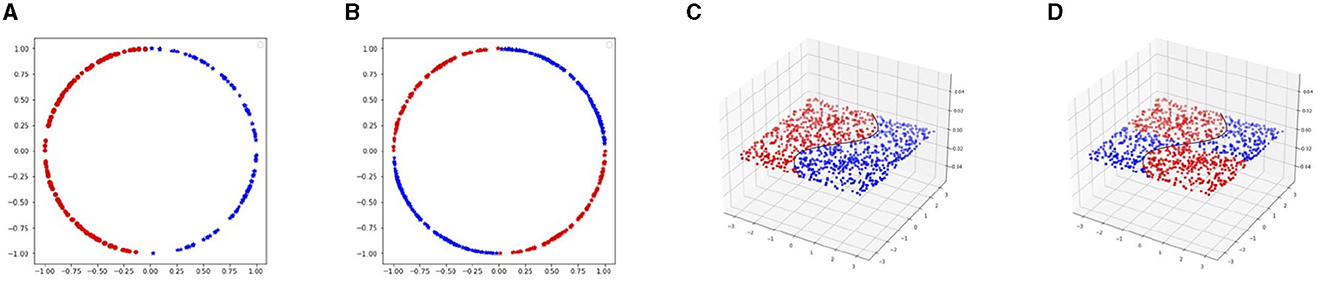
Figure 3. In this figure, we show our four toy data set. On the left side, 2D data is set on a unit circle. The single decision boundary data are linearly separated by the y-axis. Moreover, in the double decision boundary case, the circle is separated into four parts with x-axis and y-axis. On the right side, the 3D data is set. The data are distributed in a square area on x1x2-plane. In the single decision boundary example, the data are divided by the curve x1 = sin(x2). Moreover, in the double decision boundary situation, we add the y-axis as the extra boundary. (A) 2D single decision boundary. (B) 2D double decision boundary. (C) 3D single decision boundary. (D) 3D double decision boundary.
In the 3D case, we set the manifold to be and generate training data in region [−π, π] × [−π, π] on x1x2-plane. We set
Figures 3C, D show these two cases. For the single decision boundary example, due to the manifold being flat, we have Δ = ∞, and we explore the ϵ value in range [0.1, 0.8]. For the double decision boundary, the distance to the decision boundary is half of the distance in the single boundary case. Therefore, we set the range of perturbation to be [0.1, 0.4].
3.2 Algorithm for estimating different risks
To empirically estimate the decomposition of adversarial risk, we need to estimate the normal adversarial risk , the in-manifold adversarial risk , the classic adversarial risk Radv, and the standard risk Rstd. The standard risk is obtained by evaluating on the standard classifier f trained by the original training data set. For the classic adversarial risk Radv, we follow the classic approach and train the adversarial classifier fadv following the classic adversarial training Algorithm (Madry et al., 2017). The risk is evaluated on perturbed example xadv computed by the classic Projected Gradient Descent Algorithm (Madry et al., 2017). To estimate the other two risks, and , we generate adversarial perturbations along normal and in-manifold directions and use these perturbations to train different robust classifiers.
To compute the in-manifold perturbation, we design two methods. The first one is using grid search to go through all the perturbations in the manifold within the ϵ budget and return the point with maximum loss as in-manifold perturbation xin. Although this seems to be the best solution, it is quite expensive due to the grid-search procedure. Therefore, we resort to a second method in our experiments using Projected Gradient Descent (PGD) method to find a general adversarial point xadv in ambient space and then project xadv back to the data manifold . In Supplementary material, we will further compare these two methods.
Next, we explain how to obtain normal direction perturbations xnor. Note that in both the 2D and 3D toy datasets, the dimension of the normal space is 1. Therefore, the normal space at point x can be represented by . Here, v is the unit normal vector and can be computed exactly in close-form in our toy data.
We list the Radv and RHS value for 2D and 3D datasets for all classifiers in Tables 1, 2.
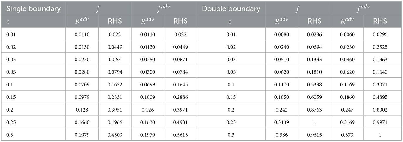
Table 1. 2D adversarial risk comparison.
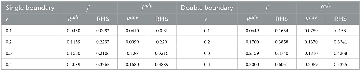
Table 2. 3D adversarial risk comparison.
3.3 Empirical results and discussion
2D dataset: We generate 1,000 2D training data uniformly. The classifier is a two-layer feed-forward network. Each classifier is trained with Stochastic Gradient Descent (SGD) with a learning rate of 0.1 for 1,000 epochs. In addition, since Δ = 1 for the unit circle, the upper bound of ϵ value is up to 1. Hence, we run experiments for ϵ from 0.01 to 0.3. We leave more discussion and visualization of this phenomenon in Supplementary material. The right hand side values of the inequality for all three classifiers are presented in Table 1. We could observe that the upper bounds hold for 2D data, at least for all these classifiers.
3D dataset: We generate 1,000 training data from the data set. The classifier is a four-layer feedforward network. We use SGD with a learning rate of 0.1 and weight decay of 0.001 to train the network. The total training epoch is 2,000. In Table 2, we list same classifiers trained on the 3D dataset. Similar to the 2D dataset, for all classifiers, inequality 1 holds. Due to the limit of the space, we provide additional empirical results in Supplementary material.
4 Experiment: real-world datasets
In this section, we verify our theoretical results on real-world dataset experiments. The challenge is to find a manifold representation and generate in-manifold/normal perturbations. We use an Autoencoder to represent the manifold. Next, we use the TNAR algorithm to generate in-manifold perturbations. We also extend TNAR to generate normal perturbations. These in-manifold/normal perturbations allow us to estimate different risks.
In Section 4.1, we explain how to learn the manifold representation. In Sections 4.2 and 4.3, we provide details on finding in-manifold and normal adversarial perturbation, respectively. Finally, in Section 4.4, we validate our theoretical bound.
Datasets: We utilize three commonly used datasets, two of which are grayscale: MNIST and FashionMNIST. Both of these datasets comprise 28×28 pixel images. MNIST dataset contains handwritten digits ranging from 0 to 9, each labeled accordingly. The dataset is divided into 60,000 training samples and 10,000 testing samples. FashionMNIST dataset consists of images of clothing items, with each item labeled into one of ten different categories. It includes 60,000 training samples and 10,000 testing samples. In addition to the grayscale datasets, we also incorporate one color dataset. SVHN dataset contains 10 different classes of digit images, each with 3×32×32 pixels.
Classifier: We selected ResNet18 as our classifier and employed the Adam optimizer with learning rate to be 0.001 for our experiments. To train the ResNet18 network for each dataset, we continued training until the training accuracy reached 99%. On the MNIST dataset, our trained classifier achieved an test accuracy of 99.24%. When applied to the FASHIONMNIST dataset, the classifier demonstrated a test accuracy of 94.78%. Moreover, the SVHN dataset obtain a test accuracy of 96.74%.
Classic adversarial training: To evaluate the robustness of the classifier, we generated Projected Gradient Descent (PGD) (Madry et al., 2017) attacks using L2 norms. For creating an adversarial attack, we set the L2 attack budget to 1.5 for the MNIST and FASHIONMNIST datasets and 0.25 for SVHN. For L∞ attacks, the perturbation budget was set to 0.3 for grayscale datasets and 8/255 for color images.
4.1 Approximation of data manifold
We employed an autoencoder structure consisting of 7 VGG blocks to approximate the underlying data manifold. The autoencoder was trained using Mean Square Loss of 400 epochs.
The output of the trained autoencoder is presented in Figure 4. We observe that for MNIST and FASHIONMNIST datasets, the reconstruction results are very close to the input data. For the SVHN dataset, while the reconstruction images are reasonably close to the input images, the reconstruction error is relatively large. We provide quantitative measures of the reconstruction quality in the Supplemental material.
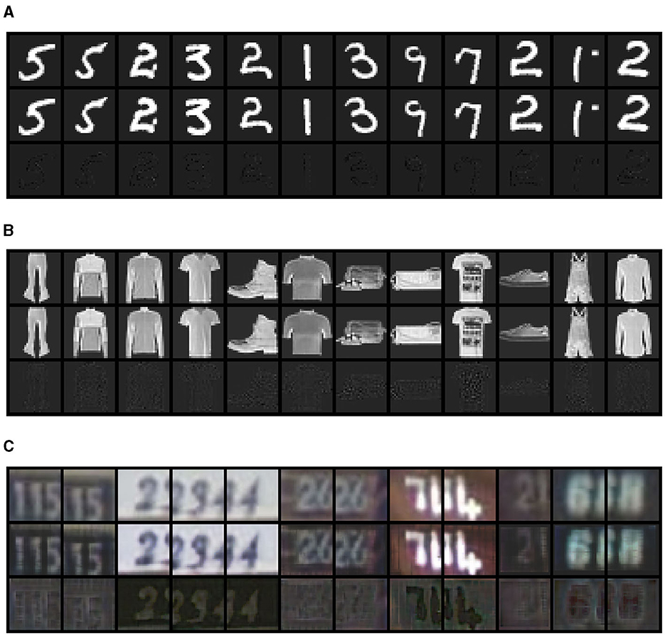
Figure 4. The manifold reconstruction from VGG-like Autoencoder Network on (A) MNST, (B) FASHIONMNST, and (C) SVHN datasets. For each dataset, we randomly sampled 12 examples. We plot the reconstructed images in the first row, the original input images in the middle row, and the difference between them in the last row.
4.2 Generating in-manifold perturbations
We use TNAR (Yu et al., 2019) to generate in-manifold examples. TNAR formulates the in-manifold adversarial attack as a linear optimization problem. Using power iteration and conjugate gradient algorithms, the tangent direction along the data manifold is identified. Next, a search along the tangent direction is performed to find valid Lp-norm adversarial perturbations.
Figure 5 shows the in-manifold perturbations generated using the TNAR method. Similar to commonly believed, the in-manifold perturbations are mainly “semantical”. We observe that the perturbations mainly occur at the edges of the image content for datasets such as MNIST or inside the items to change their texture or details, as observed in FASHIONMNIST. In the case of SVHN, the perturbations are primarily focused on the background part of the images to reshape the meaning of the digits.
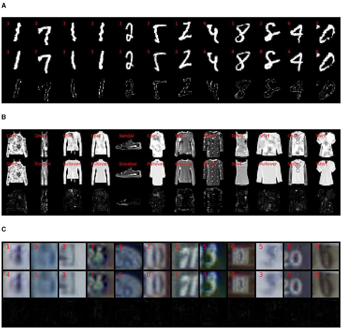
Figure 5. We present the in-manifold examples in the first row, followed by the original images in the second row, and the differences are shown in the last row. Clearly, for MNIST (A) and FASHIONMNIST (B) datasets, the attacks only affect the object part. As for SVHN (C), visualizing the difference between attacks on the object and the background is challenging. Nonetheless, when comparing with Figure 6, we can discern that the perturbations contain some information about the target object. For instance, in the eighth example, the attack mainly targets the object representing the number five and modifies it to be the number three. Moreover, in cases where multiple numbers are present in the image, such as the fifth example, the attack first merges the number two into the background and alters the appearance of the number six to be an eight.
4.3 Generating normal perturbations
We extend TNAR to compute the normal direction perturbation. In the original TNAR, a single random normal direction is generated without fully exploring the vast ambient space. However, by no means, the normal space is one-dimensional. We need to explore the whole normal space to find good normal perturbations. To this end, we employ an iterative process to repeatedly generate normal vectors. Along each normal vector, we perform a search until the perturbation limit is reached. This iterative process is crucial, and it enables us to explore the whole normal space, test a broader range of perturbation patterns, and increase the chance of obtaining better normal adversarial perturbations.
Sample normal perturbations are presented in Figure 6. Consistent with our initial expectations, the normal perturbations do not directly modify the meaning of the image. Instead, they add noise to various parts of the images, effectively deceiving the classifier.
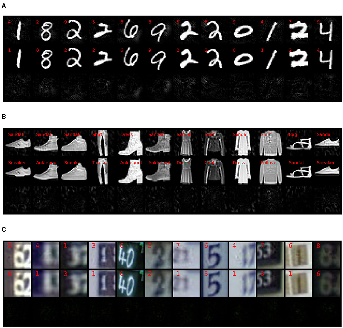
Figure 6. In this plot, we display the normal examples using the same visualization approach as the in-manifold examples. From the observation, it is evident that the attacks primarily occur in the background and lack substantial information about the target object. (A) MNIST. (B) FASHIONMNIST. (C) SVHN.
For the MNIST dataset, we observed that the normal perturbations primarily occur in the background, an area that in-manifold attacks would not typically alter. Similarly, in the FASHIONMNIST dataset, the attack expands to the background areas as well. On the other hand, for SVHN, the noise covers the entire images, not restricted to the background of the digits as the in-manifold perturbations.
4.4 Validate our theoretical findings
In this section, we validate the inequality on the classifiers. We focus on L2 normal attacks. We employ PGD attack with 40 search steps. As shown in Table 3, we report in column 1 the adversarial risk, which is the left-hand side (LHS) of Inequality 2. In columns 2, 3, and 4, we report the standard risk, in-manifold perturbation risk (evaluated on in-manifold perturbations), and normal adversarial risk (evaluated on normal perturbations). In column 5, we report their sum. Unfortunately, we have no close-form solution of the NNR term (the forth term in RHS). So, we know that column 5 is smaller than the actual RHS of the inequality.
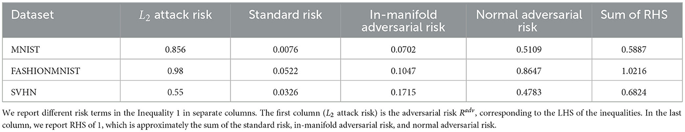
Table 3. In the table, we validate our theoretical findings using L2 norm.
Upon examining the table, we find that our theoretical findings hold for the FASHIONMNIST and SVHN datasets; the first column is smaller than the fifth column, which is smaller than the RHS. These results validate our theoretical result.
We do not observe similar trend in MNIST; the fifth column is smaller than the first column. This could be due to two potential reasons: (1) the missing term NNR is very large, causing the fifth column to be small while the actual RHS is still larger than LHS; (2) we underestimated the in-manifold and normal adversarial risks, as we are unable to find good quality in-manifold/normal perturbations. The second potential issue might be related to the separation of classes in MNIST.
4.5 Limitations and future work
Our empirical experiments are limited to low-dimensional datasets due to the computational complexity of the TNAR algorithm, which is used to find the normal and in-manifold directions. The TNAR algorithm employs power iteration to compute the approximation of the largest eigenvector of the Jacobian matrix of the network. As the dimension of input images increases, the computation complexity of generating the normal and in-manifold directions grows quadratically. This would be costly to compute for high-resolution datasets, as the computations are performed on CPU instead of GPU. Therefore, addressing the application of our approach to high-dimensional datasets is a future direction worth exploring further.
Extending our experiments to high-dimensional datasets for future studies would provide valuable insights into the generalizability and effectiveness of our approach in real-world scenarios. Additionally, investigating the behavior of the normal and in-manifold directions in high-dimensional spaces could shed light on the robustness of the proposed method against more complex and diverse adversarial attacks.
5 Conclusion
In this study, we study the adversarial risk of the machine learning model from the manifold perspective. We report theoretical results that decompose the adversarial risk into the normal adversarial risk, the in-manifold adversarial risk, and the standard risk with the additional Nearby-Normal-Risk term. We present a pessimistic case suggesting that the additional Nearby-Normal-Risk term can not be removed in general. Our theoretical analysis suggests a potential training strategy that only focuses on the normal adversarial risk.
Data availability statement
The original contributions presented in the study are included in the article/Supplementary material, further inquiries can be directed to the corresponding authors.
Author contributions
WZ: Writing – original draft. YZ: Writing – original draft. XH: Writing – original draft. YY: Writing – review & editing. MG: Writing – review & editing. CC: Writing – review & editing. DM: Writing – review & editing.
Funding
The author(s) declare financial support was received for the research, authorship, and/or publication of this article. MG would like to acknowledge support from the US National Science Foundation (NSF) 476 awards CRII-1755791 and CCF-1910873. This material is partially based on study supported by the Defense Advanced Research Projects Agency (DARPA) under Agreement No. HR0011-22-9-0077. Any opinions, findings, and conclusions or recommendations expressed in this material are those of the author(s) and do not necessarily reflect the views of DARPA. The content of this manuscript has been presented at the AISTATS (Zhang et al., 2022).
Conflict of interest
The authors declare that the research was conducted in the absence of any commercial or financial relationships that could be construed as a potential conflict of interest.
The author(s) declared that they were an editorial board member of Frontiers, at the time of submission. This had no impact on the peer review process and the final decision.
Publisher's note
All claims expressed in this article are solely those of the authors and do not necessarily represent those of their affiliated organizations, or those of the publisher, the editors and the reviewers. Any product that may be evaluated in this article, or claim that may be made by its manufacturer, is not guaranteed or endorsed by the publisher.
Supplementary material
The Supplementary Material for this article can be found online at: https://www.frontiersin.org/articles/10.3389/fcomp.2023.1274695/full#supplementary-material
References
Awasthi, P., Dutta, A., and Vijayaraghavan, A. (2019). “On robustness to adversarial examples and polynomial optimization,” in Advances in Neural Information Processing Systems, 32.
Carlini, N., and Wagner, D. (2017). “Towards evaluating the robustness of neural networks,” in 2017 IEEE Symposium on Security and Privacy (sp) (New York, NY: IEEE), 39–57.
Carmon, Y., Raghunathan, A., Schmidt, L., Liang, P., and Duchi, J. C. (2019). Unlabeled data improves adversarial robustness. arXiv.
Cayton, L. (2005). Algorithms for Manifold Learning. San Diego: University of California at San Diego Tech. Rep, 1.
Dey, T. K., and Goswami, S. (2006). Provable surface reconstruction from noisy samples. Comp. Geomet. 35, 124–141. doi: 10.1016/j.comgeo.2005.10.006
Dohmatob, E. (2019). “Generalized no free lunch theorem for adversarial robustness,” in International Conference on Machine Learning (London: PMLR), 1646–1654.
Edelsbrunner, H., and Shah, N. R. (1994). “Triangulating topological spaces,” in Proceedings of the Tenth Annual Symposium on Computational Geometry (New York, NY: Association for Computing Machinery), 285–292.
Fawzi, A., Fawzi, H., and Fawzi, O. (2018). “Adversarial vulnerability for any classifier,” in Advances in Neural Information Processing Systems, 31.
Gilmer, J., Metz, L., Faghri, F., Schoenholz, S. S., Raghu, M., Wattenberg, M., et al. (2018). Adversarial spheres. arXiv.
Gowal, S., Qin, C., Uesato, J., Mann, T., and Kohli, P. (2020). Uncovering the limits of adversarial training against norm-bounded adversarial examples. arXiv.
Guo, M., Yang, Y., Xu, R., Liu, Z., and Lin, D. (2020). “When nas meets robustness: In search of robust architectures against adversarial attacks,” in Proceedings of the IEEE/CVF Conference on Computer Vision and Pattern Recognition (New York, NY: IEEE), 631–640.
He, K., Zhang, X., Ren, S., and Sun, J. (2016). “Deep residual learning for image recognition,” in Proceedings of the IEEE conference on computer vision and pattern recognition (New York, NY: IEEE), 770–778.
Krizhevsky, A., Sutskever, I., and Hinton, G. E. (2012). Imagenet classification with deep convolutional neural networks. Adv. Neural Inform. Proc. Syst. 25, 1097–1105. doi: 10.1145/3065386
Lau, C. P., Liu, J., Souri, H., Lin, W.-A., Feizi, S., and Chellappa, R. (2023). Interpolated joint space adversarial training for robust and generalizable defenses. IEEE Trans. Pattern Anal. Mach. Intell. 45, 13054–13067. doi: 10.1109/TPAMI.2023.3286772
Levine, S., and Abbeel, P. (2014). “Learning neural network policies with guided policy search under unknown dynamics,” in NIPS (Pittsburgh: CiteSeerX), 1071–1079.
Lin, W.-A., Lau, C. P., Levine, A., Chellappa, R., and Feizi, S. (2020). Dual manifold adversarial robustness: Defense against lp and non-lp adversarial attacks. Adv. Neural Inform. Proc. Syst. 33, 3487–3498.
Madry, A., Makelov, A., Schmidt, L., Tsipras, D., and Vladu, A. (2017). Towards deep learning models resistant to adversarial attacks. arXiv preprint.
Nagabandi, A., Kahn, G., Fearing, R. S., and Levine, S. (2018). “Neural network dynamics for model-based deep reinforcement learning with model-free fine-tuning,” in 2018 IEEE International Conference on Robotics and Automation (ICRA) (New York, NY: IEEE), 7559–7566.
Narayanan, H., and Mitter, S. (2010). “Sample complexity of testing the manifold hypothesis,” in Proceedings of the 23rd International Conference on Neural Information Processing Systems (Red Hook, NY: Curran Associates Inc.), 1786–1794.
Niyogi, P., Smale, S., and Weinberger, S. (2008). Finding the homology of submanifolds with high confidence from random samples. Discrete & Comp. Geomet. 39, 419–441. doi: 10.1007/s00454-008-9053-2
Raghunathan, A., Xie, S. M., Yang, F., Duchi, J., and Liang, P. (2020). “Understanding and mitigating the tradeoff between robustness and accuracy,” in Proceedings of the 37th International Conference on Machine Learning, 7909–7919.
Rice, L., Wong, E., and Kolter, Z. (2020). “Overfitting in adversarially robust deep learning,” in International Conference on Machine Learning (London: PMLR), 8093–8104.
Rifai, S., Dauphin, Y. N., Vincent, P., Bengio, Y., and Muller, X. (2011). The manifold tangent classifier. Adv. Neural Inform. Proc. Syst. 24, 2294–2302.
Saul, L. K., and Roweis, S. T. (2003). “Think globally, fit locally: unsupervised learning of low dimensional manifolds,” in Departmental Papers (CIS) (Brookline, MA: Microtome Publishing), 12.
Shafahi, A., Najibi, M., Ghiasi, A., Xu, Z., Dickerson, J., Studer, C., et al. (2019). Adversarial training for free! arXiv.
Shaham, U., Yamada, Y., and Negahban, S. (2018). Understanding adversarial training: increasing local stability of supervised models through robust optimization. Neurocomputing 307, 195–204. doi: 10.1016/j.neucom.2018.04.027
Shamir, A., Melamed, O., and BenShmuel, O. (2021). “The dimpled manifold model of adversarial examples in machine learning,” in Advances in Neural Information Processing Systems, 30.
Stutz, D., Hein, M., and Schiele, B. (2019). “Disentangling adversarial robustness and generalization,” in Proceedings of the IEEE/CVF Conference on Computer Vision and Pattern Recognition (New York, NY: IEEE), 6976–6987.
Su, D., Zhang, H., Chen, H., Yi, J., Chen, P.-Y., and Gao, Y. (2018). “Is robustness the cost of accuracy?-A comprehensive study on the robustness of 18 deep image classification models,” in Proceedings of the European Conference on Computer Vision (ECCV) (Berlin: Springer Science+Business Media), 631–648.
Szegedy, C., Zaremba, W., Sutskever, I., Bruna, J., Erhan, D., Goodfellow, I., et al. (2013). Intriguing properties of neural networks. arXiv.
Tanay, T., and Griffin, L. (2016). A boundary tilting persepective on the phenomenon of adversarial examples. arXiv.
Tenenbaum, J. B., De Silva, V., and Langford, J. C. (2000). A global geometric framework for nonlinear dimensionality reduction. Science 290, 2319–2323. doi: 10.1126/science.290.5500.2319
Tsipras, D., Santurkar, S., Engstrom, L., Turner, A., and Madry, A. (2018). Robustness may be at odds with accuracy. arXiv.
Vaswani, A., Shazeer, N., Parmar, N., Uszkoreit, J., Jones, L., Gomez, A. N., et al. (2017). “Attention is all you need,” in Advances in Neural Information Processing Systems, 30.
Wu, Y., Schuster, M., Chen, Z., Le, Q. V., Norouzi, M., Macherey, W., et al. (2016). Google's neural machine translation system: bridging the gap between human and machine translation. arXiv.
Xie, C., Tan, M., Gong, B., Wang, J., Yuille, A. L., and Le, Q. V. (2020). “Adversarial examples improve image recognition,” in Proceedings of the IEEE/CVF Conference on Computer Vision and Pattern Recognition (New York, NY: IEEE), 819–828.
Yang, Y.-Y., Rashtchian, C., Zhang, H., Salakhutdinov, R., and Chaudhuri, K. (2020). A closer look at accuracy vs. robustness. Adv. Neural Inform. Proc. Syst. 33, 8. doi: 10.1007/978-3-030-63823-8
Yu, B., Wu, J., Ma, J., and Zhu, Z. (2019). “Tangent-normal adversarial regularization for semi-supervised learning,” in Proceedings of the IEEE/CVF Conference on Computer Vision and Pattern Recognition (New York, NY: IEEE), 10676–10684.
Zhang, H., Yu, Y., Jiao, J., Xing, E., El Ghaoui, L., and Jordan, M. (2019). “Theoretically principled trade-off between robustness and accuracy,” in International Conference on Machine Learning (London: PMLR), 7472–7482.
Keywords: robustness, adversarial attack, manifold, topological analysis of network, generalization
Citation: Zhang W, Zhang Y, Hu X, Yao Y, Goswami M, Chen C and Metaxas D (2024) Manifold-driven decomposition for adversarial robustness. Front. Comput. Sci. 5:1274695. doi: 10.3389/fcomp.2023.1274695
Received: 08 August 2023; Accepted: 19 December 2023;
Published: 11 January 2024.
Edited by:
Pavan Turaga, Arizona State University, United StatesReviewed by:
Jiang Liu, Johns Hopkins University, United StatesChun Pong Lau, City University of Hong Kong, Hong Kong SAR, China
Copyright © 2024 Zhang, Zhang, Hu, Yao, Goswami, Chen and Metaxas. This is an open-access article distributed under the terms of the Creative Commons Attribution License (CC BY). The use, distribution or reproduction in other forums is permitted, provided the original author(s) and the copyright owner(s) are credited and that the original publication in this journal is cited, in accordance with accepted academic practice. No use, distribution or reproduction is permitted which does not comply with these terms.
*Correspondence: Chao Chen, chao.chen.1@stonybrook.edu; Dimitris Metaxas, dnm@cs.rutgers.edu