Developing an Error Map for Cognitive Navigation System

1. Introduction

Many types of navigation services, such as applications on smartphones and automotive navigation systems, are becoming popular. These services play an important role in intelligent transportation systems (ITSs). However, they require highly accurate positioning, especially in urban areas. One technology that is important for providing location information such as latitude and longitude is the Global Navigation Satellite System (GNSS). Position information determined by GNSS usually is inaccurate by a few meters or more, and research has been performed to reduce the error. One promising technology for acquiring accurate location data is real-time kinematic (RTK) positioning (Sakai, 2003). In the best-case scenario, RTK positioning can provide location information with an error of only a few centimeters. Owing to its low cost and small size, the RTK positioning device is expected to be used widely. However, its positioning accuracy is not good where signal reception from satellites is unstable, especially in urban canyons. RTK accuracy depends on the environment, such as when buildings shadow signals from a GNSS satellite, so it is difficult to realize accurate navigation with RTK positioning in a city's downtown area. One solution for solving the challenges in an urban environment is to select a satellite to eliminate signal shading by buildings. An elevation angle mask (Misra and Enge, 2001) is a technique that provides accurate position information in cities by employing satellites that exist at higher-elevation angle spaces. However, such methods for selecting satellites sometimes reduce the number of usable satellites, so accuracy does not increase as expected. Therefore, the accuracy of GNSS positioning in urban areas is challenging in general.

However, we believe that there is an alternative approach wherein applying a cognitive methodology provides user satisfaction for services such as car navigation. The main stream of the research on GNSS is increasing accuracy. However, we sometimes have a problem of car navigation because of low accuracy of position. If the positioning accuracy is not good because of the conditions, we expect that a navigation application provides an optimal solution. For example, if the accuracy of position is not good, a navigation system can lead a user to a location where the accuracy is better. We would like to call such navigation system as a cognitive navigation system. Therefore, we would like to apply the Cognitive Infocommunications (CogInfoCom) approach (Baranyi and Csapo, 2012; Baranyi et al., 2015). This idea extends human cognitive capabilities and would even enable life support.

Figure 1 shows the CogInfoCom concept for a location-based service (LBS). The original CogInfoCom architecture is shown in Figure 1 (left). A communication device offers an opportunity for users to interact with the environment by using a network and an autonomous cognitive system with sensors and Internet of Things devices. Figure 1 (right) depicts one implementation of the CogInfoCom system to an LBS, namely, an automotive navigation system. Clearly, LBSs are one of the most important services and are strongly affected by situations. In this implementation, we introduce an error map (Figure 2) that offers a level of error for GNSS positioning to improve navigation if the GNSS signal is weak or noisy. CogInfoCom makes an environment intelligent and provides information automatically.

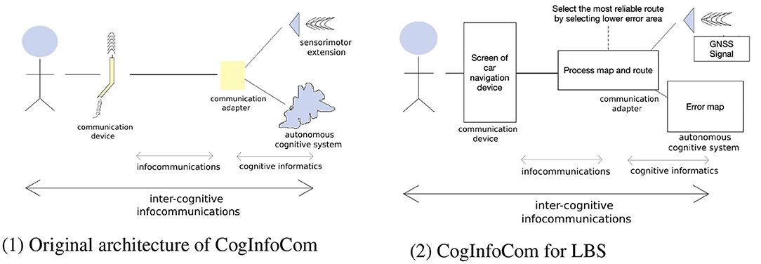
Figure 1. Error mapping for the CogInfoCom architecture.

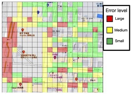
Figure 2. An example of an error map.

In the next section, we propose a new technique that increases the accuracy of GNSS positioning and the usability of LBSs by providing the error level of a specific location. We mention the difficulty of GNSS positioning and related works such as techniques for multipath shadowing environments or multi-GNSS receivers. Section 3 discusses the objectives of this research, and section 4 presents the pre-examination results to explain the characteristics of the GNSS positioning error. In section 5, details of the proposed method are discussed. The proposed methods are evaluated in section 6, and examples of how to apply the error map are proposed in section 7. Finally, section 8 concludes and discusses further studies.

2. Problems and Related works

2.1. Characteristics of the GNSS Error

As described in the previous section, one of the issues related to reducing the accuracy of GNSS is errors. A GNSS positioning error can occur for several reasons. Such an error can be caused by any of the following: the satellite's clock, the orbit of a satellite, noise from the convection of air in the ionosphere, noise of a GNSS receiver, or multipaths (Sakai, 2003). An error that is caused by a clock's satellite or the satellite's orbit relates to the satellite itself, so it is possible to reduce the error if more than two receivers obtain a signal from the same satellite. In widely used techniques such as the Saastamoinen model (Saastamoinen, 1973a,b,c) and the Klobuchar model (Klobuchar, 1987), an error caused by noise from the GNSS receiver depends on the baseline (Satirapod and Chalermwattanachai, 2005). Therefore, it is possible to remove the miscalculation as a common error if there are two neighbor receivers. The remaining error depends on shadows, which cause reflections and increase the signal paths from GNSS satellites, and such reflections interfere with the original signal. Such an error varies, depending on the environment, and is difficult to predict. Also, the objects' shadows reduce the number of GNSS satellites from a particular receiver that secures the signal and increases error. The shadowing environment causes errors that are difficult to remove, and the levels of error depend on the environment. Therefore, it is important to handle these types of errors for an LBS.

2.2. Coordinated Positioning

One approach for reducing errors is coordinated positioning, which minimizes miscalculations that are caused by sharing information among several receivers. The idea is similar to RTK positioning and removing the common receiver errors. The coordinated positioning can detect multipaths and eliminate the satellite that causes them (Osechas et al., 2015) to increase accuracy. A Differential Global Positioning System (DGPS) is one type of coordinated positioning. The reference station distributes correction information to neighboring receivers. Accordingly, a simplified DGPS is proposed (Miyata et al., 1996; Miyata and Sakitani, 1997). This system offers accurate positioning data by processing the cross-correlation of positioning data of two receivers. There is also a method for grouping the characteristics of GNSS receivers, such as an error-reduction method for the receivers that move together (Odaka et al., 2011) and to reduce multipaths by using numerous antennas on an automobile (Kubo et al., 2017).

2.3. Error Correction by a Map

A map is an important parameter for increasing the positioning accuracy and provides both correction and height information (Iwase et al., 2013). The information provided by a map is increasing, such as 3D maps. We also propose a method to provide DGPS correction data by combining map information and the location of an automobile (Rohani et al., 2016).

3. Estimating the Error of GNSS

In this section, we present the results of an experiment that considers a method to determine an estimated position error. As explained in the previous section, it is difficult to eliminate errors caused by a multipath. Table 1 presents the methods used in previous studies. These methods used the pseudorange. However, for a low-cost GNSS device such as a smartphone, the positioning function is a black box, and it is difficult to see the pseudorange information. Therefore, it is necessary to use only position data, with no internal data from the GNSS receiver. A way to use the group characteristics of GNSS receivers is to apply only the position data. However, because it is assumed to be stationary, it requires developing an error-reduction method that uses only the mobile receiver's position data. We have been developing some methods to reduce errors that relate to multipath under the restrictions mentioned. In the remainder of this section, we will discuss our methods.

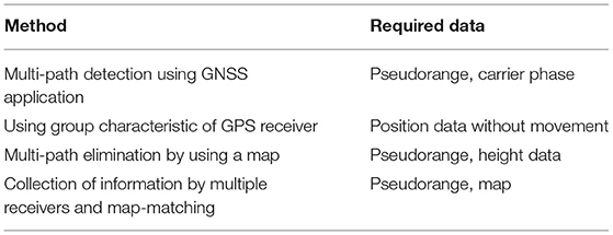
Table 1. Related works.

3.1. Method 1: Using the Common Temporal Error

We studied a method that focuses on how a common temporal error occurs in nearby receivers for the GNSS (Nakamura, 2018). The delay due to the convection of air in the ionosphere causes the main GNSS positioning error. If the distance between two receivers is small, both have the same effect caused by the delay due to the convection of air in the ionosphere and may have a common error. However, if each receiver obtains a signal from a different GNSS satellite, the pseudorange should vary and have different error patterns. Therefore, it is necessary to use the same GNSS satellite. To prove the effectiveness of this idea, we designed a system model (Figure 3) and performed a trial. As a result, accuracy improved by 0.5–1.6 m.

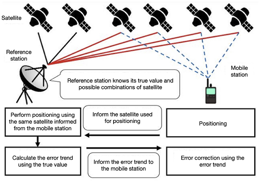
Figure 3. System model of using a common temporal error.

3.2. Method 2: Using a Bias of the Positioning Error by Multipath

This idea uses an error bias caused by multipath between neighboring receivers. In our previous research (Kitani et al., 2012), the error of neighboring receivers is biased. In this method, two receivers were placed on top of the roof of a car with the same distance, and the error of position was observed. This automobile was moving straight, and the environment alternates between not being in shadow and being in shadow. If the observed error of the two receivers fluctuates widely, both are affected for the same reason. In this case, we can understand that both receivers are affected by multipath, and we can add a corrected point by using a previously accurate result in the shadowed environment.

3.3. Method 3: Error Map

Methods 1 and 2 were designed to reduce errors. However, our idea is different in that if we know the location is shadowed and what the possible error level is, we can adapt the situation. We would like to propose a new idea, an error map, for that purpose. Figure 2 shows an example of an error map in which different colors display the multipath's level of error. For example, if we know that the location has a poor error level, we can either change a shadow mask to eliminate the low-accuracy satellite or select a route with a better error level.

3.4. Comparing the Methods

In what follows, we compare the three proposed methods.

• Method 1 uses a common temporal error and has value for correcting an error by using position information. However, this technique applies to locations without shadowing. Also, if both the reference station and the mobile terminal are in a shadowy condition, it is possible to remove the error. The reference station is usually located at a position without a shadow, so it is not useful in the usual case.

• Method 2, which uses the bias of the positioning error by multipath, is useful in a limited situation, since a case with a similar multipath trend is rare.

• In Method 3, the error map is not useful for removing the error. This method can change the shadow mask to reduce errors. However, when using this technique, a participant can choose various ways that are not affected by the GNSS positioning error. The error map can also provide information to improve the infrastructure, such as a beacon to provide location information in an urban area, such as a dynamic traffic map (Watanabe et al., 2020). We believe that this method provides many possibilities to develop LBSs.

Accordingly, we selected the Method 3 error map because of the research target since the method can be applied to the LBSs. The following are the objectives of this research.

• Requirement 1: To develop a function to estimate the error, with a 1 m target for 90% of the cases

• Requirement 2: To cultivate a function to decide the error level, with a target of 90% success rate at the error-level decision.

4. Pre-Experiment

We performed the following two pre-experiments to evaluate the error size by using two GNSS receivers and their position.

• Pre-experiment 1: observing the trend of positioning results affected by multipath measured in both shaded and unshadowed environments by using two GNSS receivers (stationary)

• Pre-experiment 2: the same test but in the moving case.

4.1. Evaluating Pre-experiment 1

We performed pre-experiment 1 to observe how the trend of positioning results of moving two receivers that are affected by multipath was measured under shaded and unshadowed environments. The experimental factors are shown in Table 2 (1). The reference station was not shadowed. The user's receiver was shadowed and affected by multipath and was located close to the large building, with a distance of approximately 20 m.

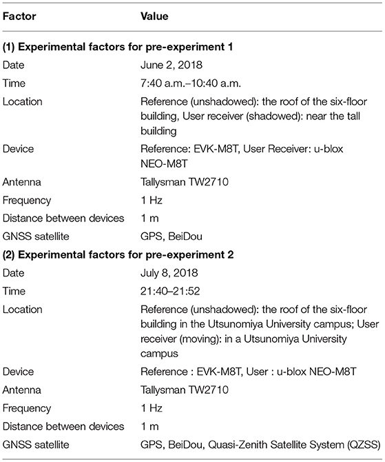
Table 2. Experimental factors for pre-experiment 1 and 2.

In this experiment, true value is defined as the average of the fixed solution. The distance between the two receivers at the unshadowed environment was 0.947 m, whereas that in the shadowed environment was 0.247 m. Since the real distance was 1 m, the result of the shadowed environment was not good. Also, in the unshadowed environment, some epochs do not have an output. Although there were some errors, they were not as severe. Figure 4 (1, 2) shows the error in the shadowed (light color) and unshadowed (dark color) environments at point a, whereas Figure 4 (3, 4) shows the error at point b. If there is no miscalculation, the difference should be 0. The error in the shadowed environment is larger than that in the unshadowed one. The error trend is changing slowly and extensively. From this experiment, we predict that in the shadowed environment, the noise increases. So it may be possible. The shadowed environment has an error by multipath. Also, since the miscalculation trend is changing slowly and significantly in the shadowed environment, we believe that the effect of satellite constellation is more significant than that in the unshadowed environment.

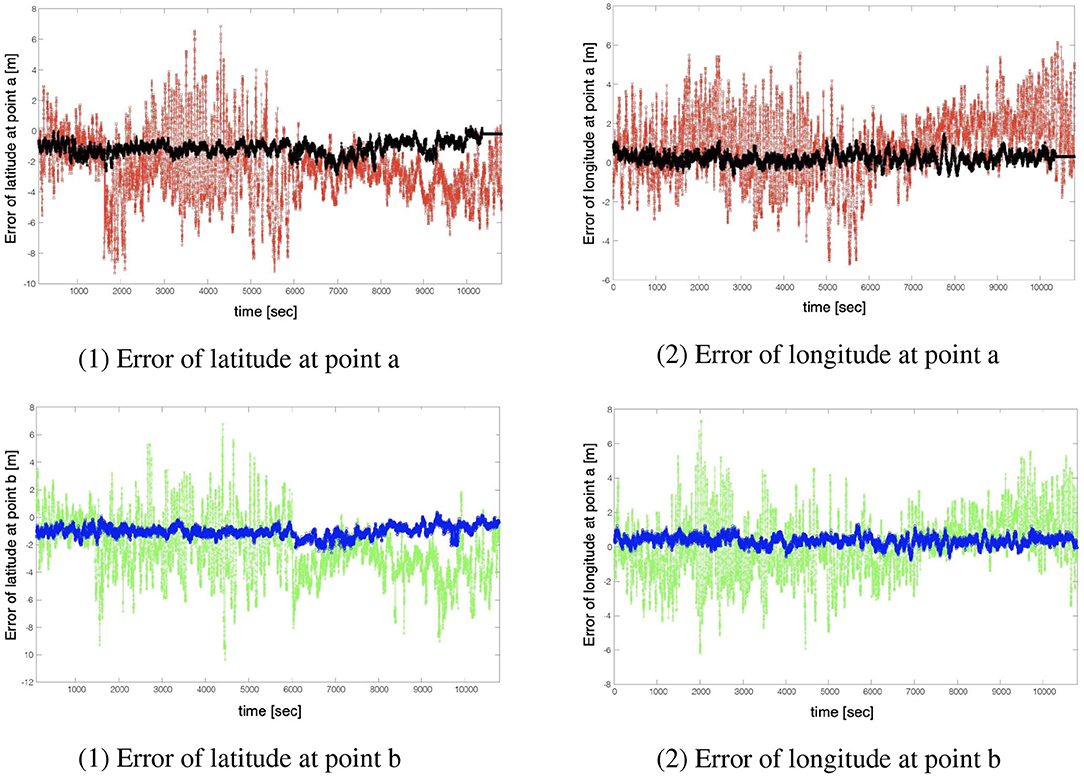
Figure 4. Results at point a and b of pre-experiment 1.

4.2. Evaluating Pre-experiment 2

We performed the next experiment to observe the trend of the positioning results of moving two receivers affected by multipath. We examined the relationship between the average error of the position of each receiver and the distance from the receivers. We set two receivers on a push car, which moved to Utsunomiya University campuses and measured the positions. The distance between receivers was 40 cm. The moving route was selected for motion in the shadowed area. Table 2 (2) shows the experimental factors. We used a fixed RTK solution as the true value and calculated the positioning error as the distance using Hubeny's formula (Vincenty, 2013) and the longitude and latitude of the receiver's true value and position.

We define the errors in two receivers as e₁ and e₂, and the average of the errors is $ē=\frac{e_1+e_2}{2}$[m]. Then, we defined the distance between two receivers as $\tilde{r}$[m], as we would like to evaluate the relationship between the average positioning error (ē) and the distance between two receivers ($\tilde{r}$). This examination was performed at the epoch, where the positioning error (e₁, e₂) and distance between receivers ($\tilde{r}$) were acquired.

Figure 5 (left) shows how if the distance between receivers ($\tilde{r}$) were increased, the average positioning error of two receivers (ē) was increased. Figure 5 (right) is an enlargement of Figure 5 (left), where the distance between receivers ($\tilde{r}$) is between 0 and 10 m. This figure shows that there are many points scattered in the positive direction of the vertical axis, but not in the negative direction. Figure 5 (left) and (right) show the distance between receivers ($\tilde{r}$) and the average positioning error of two receivers (ē), which has a positive correlation because if ē becomes larger, $\tilde{r}$ should be larger.

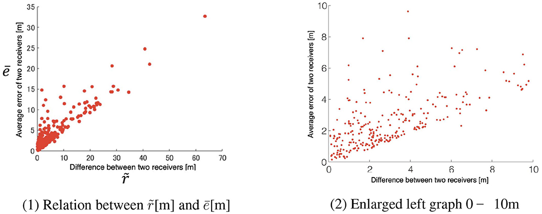
Figure 5. Relationship between the distance of two receivers and the error.

The average positioning error of two receivers (ē) requires the true value, although the distance between receivers ($\tilde{r}$) can be calculated from the positioning data of the receiver. Therefore, we believe that it is possible to calculate the average of the positioning error of two receivers (ē) from a distance between receivers ($\tilde{r}$) by using two low-cost GNSS receivers. If we can obtain the average of the positioning error of two receivers (ē), we can use that data to develop an error map.

In the next section, we explain the method to calculate the estimated positioning error.

5. The Proposed Method for Calculating the Estimated Positioning Error for the Error Map

This section presents the details of our proposed method for calculating the estimated positioning error for the error map.

5.1. Error Estimation

Figure 6 (1) depicts the parameters and Figure 6 (2) illustrates the system model for the error estimation.

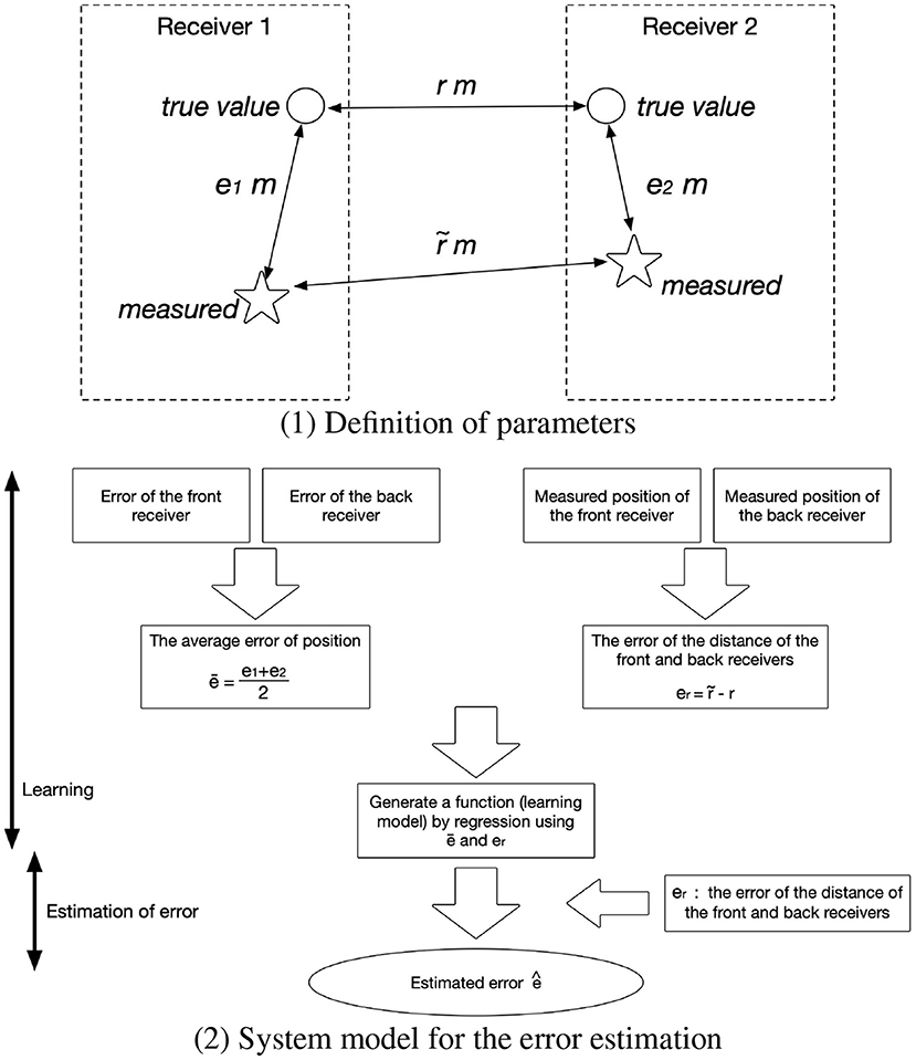
Figure 6. Definition of parameters and System model for the error estimation.

Let us assume there are two receivers located in front of and behind the roof of a car. We use the following parameters:

• e₁[m]: positioning error between the true value and the standalone positioning at the front receiver

• e₂[m]: positioning error between the true value and the standalone positioning at the back receiver

• $\tilde{r}$[m]: the measured distance between two receivers acquired from standalone positioning

• r[m]: the distance between two receivers acquired from the true value

• ē[m]: positioning error of two receivers [calculated by Formula (1)]

• e_r[m]: error of the distance of two receivers [calculated by Formula (2)].

We obtained the error estimation function by performing a regression analysis, with the front-to-back receiver distance error e_r since the x-axis and the front-and-back positioning error mean ē as the y-axis. From the shape of Figure 5 (left), we performed linear regression and trained the intercept to become 0. Subsequently, we obtained the relation between e_r and ē. Using this function, we can obtain e_r from $\tilde{r}$ using Formula (2). We can then estimate ē.

5.2. Deciding on the Magnitude of Error

We discuss the error level evaluation method (i.e., large or small) in this subsection. We also propose methods for deciding on the error level based on the discussion in the previous section. We decide that “the error is large” if the error is larger than $\tilde{r}$; otherwise, “the error is small.” However, this simple method sometimes causes an unexpected problem; hence, we would like to discuss this in detail.

5.2.1. Method Using Mileage and Distance Between Positioning Points

The method explained in the previous section has some problems when deciding on the error level. For example, the positioning point receives an error in the same direction and becomes close to the receiver distance's true value, despite receiving the error. Therefore, the distance calculated from the current time t, the time t′ of the previous epoch, and the speed v are the pseudo-true values. We can then estimate the magnitude of error by taking the difference between the current positioning point and the distance s obtained from the previous epoch's positioning point [Figure 7 (1)]. This value is the difference between the distance that should have been traveled and the distance that was traveled. Thus, we can decide on this considering the following: the error is large if the value is large, and the error is small if the value is small. Therefore, the problem mentioned at the beginning of this section can be solved in many cases. However, this solution still has issues if the positioning points appear in the vehicle's opposite direction.

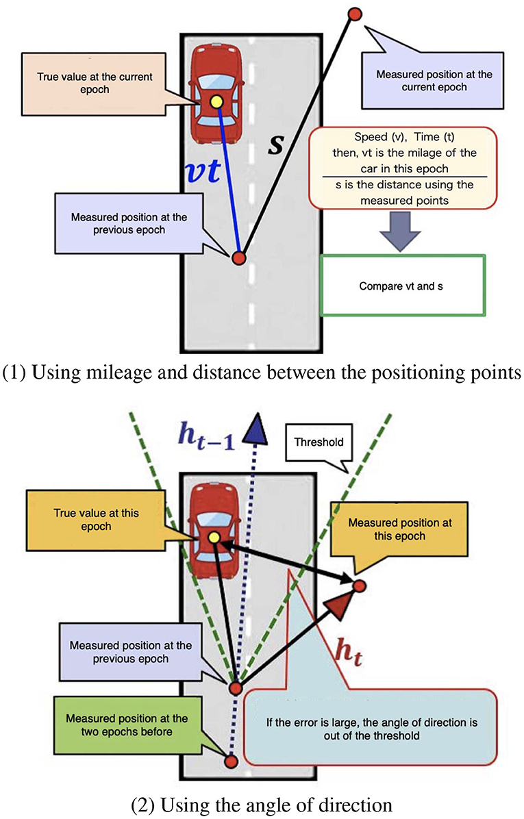
Figure 7. Error level estimation methods.

5.2.2. Method Using the Angle of Direction

We introduce a method for reinforcing the proposed method by using the angle of direction to solve the previous section's problem. This method is used as an estimation reinforcement when the vehicle is going straight on a straight road. First, the vehicle's traveling direction angle is obtained using the past two stable positioning points. Next, the threshold of the angle of the vehicle's traveling direction is set. Finally, we determine if the positioning error is small by determining whether the current epoch's positioning point is within the threshold of that angle. Figure 7 (2) presents an example. As in the lower-left part, the positioning point of the previous epoch and the vehicle's traveling direction angle determine whether the current epoch's positioning point is within the threshold. In this case, it was not within the threshold; thus, it is a “large error.”

5.2.3. Migration of the Methods

We migrate the proposed methods in this section (Figure 8). First, the distance between the two receivers is judged, and we judge whether $\tilde{r}$ exceeds 3[m]. If $\tilde{r}>3$, we judge this as a “large error.” If $\tilde{r}<3$, we judge this as a “small error.” The methods using mileage and angle of the vehicle's traveling direction are applied. If both methods answer “large error,” the result should be “large error”; otherwise, the result is “small error.”

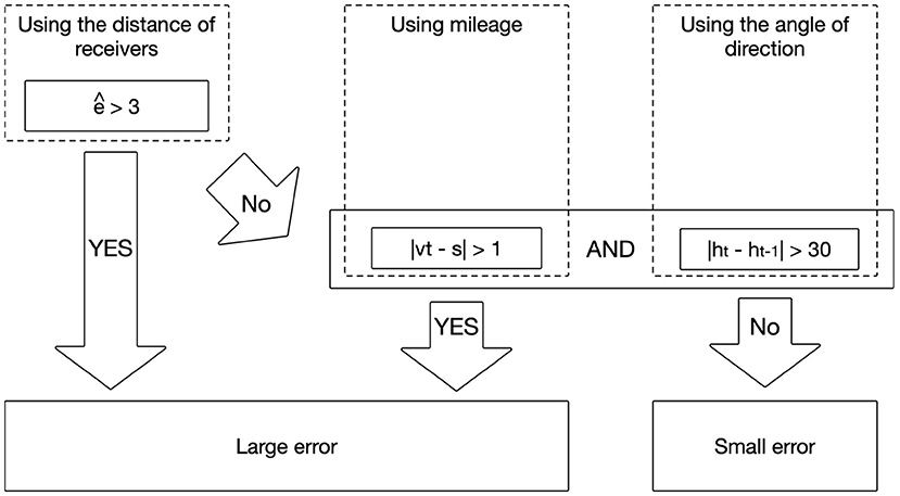
Figure 8. Migration of the methods.

6. Evaluation of the Proposed Methods

This section explains the proposed methods' evaluation results using a car with two receivers on the roof. The calculation was performed after obtaining the data.

6.1. Evaluation of the Error Estimation Method

Table 3 (1) lists the experiment factors of evaluation of the error estimation method.

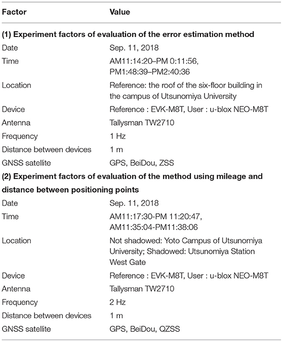
Table 3. Experiment factors of the proposed method.

Two low-priced receivers (u-blox EVK-M8T) were installed on a car roof [Figure 9 (1)]. The distance of the receivers was 1 m. The true value of the position was detected using POS LV 620 from Trimble. POS LV 620 can perform positioning with an accuracy of several centimeters by integrating an inertial measurement unit (IMU) and a DMI (odometer) in addition to a highly accurate GNSS receiver antenna.

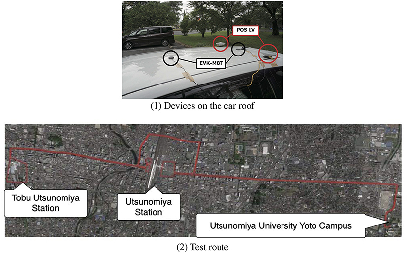
Figure 9. Devices on the car roof and test route.

Figure 9 (2) depicts the route traveled to obtain the experimental data. After leaving Utsunomiya University, Yoto Campus, the car passed through Utsunomiya Station and went to Tobu Utsunomiya Station before returning to Yoto Campus.

The regression analysis data were calculated as the error of the distance of the two receivers (e_r) and the receiver average positioning error (ē) from the data measured at 1:48:39 p.m.–2:40:36 p.m.. The data used for the evaluation were measured at 11:14:20 a.m.–01: 00: 11: 56 p.m.. We used e_r of the distance between the front and rear receivers. The error estimation value ẽ output by the function discussed in the previous section was compared with the true value. The estimated positioning error was evaluated for accuracy. The estimated error (ẽ) obtained by the proposed method was subtracted from the positioning error (e₁) of the front receiver to obtain the absolute value (i.e., |ê - e₁|) summarized as a frequency in Figure 10 (left). Figure 10 (right) depicts a similar result for the back receiver. The value of x = 10 [m] is the frequency, including all 10 m or more errors. The cumulative frequency is also displayed. A comparison of Figure 10 (left) and Figure 10 (right) shows that more than 80% of the estimated error was within 3 m (both within the front and back). Furthermore, in a common part, the epochs with errors of 1 and 2 m are the most in error estimation. The results of Figure 10 (left) are shown in Table 4 as values. The number of epochs is very small when the error is larger than 3 m. The results showed that 80% or more of the estimated error (ẽ) showed an error of 3 m or less from the actual positioning error. We think that the reason for the error of a few meters is the processed regression analysis. The intercept became 0. We also think that no perfect correlation exists in the data, as shown in Figure 5 (left). If the error e_r in the distance between the front and rear receivers became closer to 0, it became inaccurate in the former case. We think that the reason for this is that the learning process was performed. The intercept became 0. Furthermore, the latter led to the method's performance degradation because the function's incompleteness caused it due to the lack of a perfect correlation. This method can also provide a quantitative error amount. Our target was the estimated error of 1 m; however, the result that satisfied this target was approximately 20%. Hence, at this moment, our method is not suitable for a service that requires a strict error level. Our method can be used for services that do not require strict accuracy, such as notifying the user of how reliable the current positioning is.

Figure 10. Frequency of error.

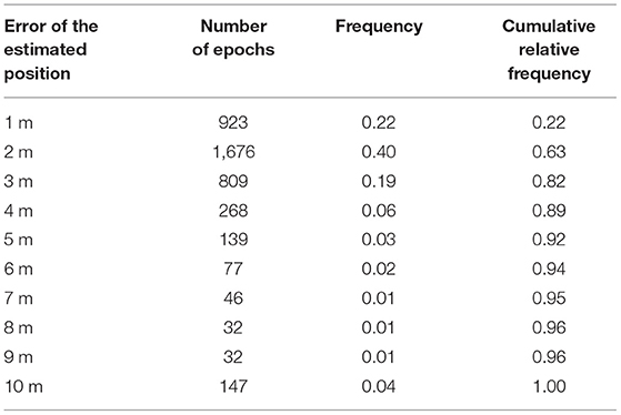
Table 4. Detailed result of frequency of error (front).

6.2. Evaluation of the Method Using Mileage and Distance Between Positioning Points

The evaluation was performed to confirm how much the error can be judged by the proposed method and how much the positioning accuracy can be improved using the "error map.' We used the same devices that we used in the previous evaluation. Table 3 (2) presents the experiment factors. In this experiment, we prepared two types of cases: one for the shadowed environment and one for the not-shadowed environment. The non-shadowed environment was set up near Utsunomiya University Yoto Campus. This area has a few high shields to the left and right of the road, and a stable positioning is possible. The shadowed environment was set up at the rotary at the west exit of Utsunomiya Station. There are many tall buildings around this area, and a pedestrian bridge covers the zenith direction. The evaluation was performed by using the method for determining the magnitude of the error and comparing it with the magnitude of the front receiver's actual error amount. After determining the magnitude of the error using this method, we confirmed whether the positioning accuracy could be improved by selecting satellites using the elevation mask. In the case of a “large error,” we predicted the positioning accuracy could be improved by selecting a high-elevation satellite that does not cause a multi-path. In the case of a “small error,” we predicted the positioning accuracy could be improved by using more satellites in such a way that the weak elevation mask would be useful. We want to verify the error map effectiveness. Table 5 (1) describes the result of the non-shadowed environment. The success rate of the judgment was 97.6%. The result showed that the error size was successfully judged with high accuracy. Almost all actual errors showed a “small error” in the epoch, which is the reason why the judgment was performed well by the method. Table 5 (2) describes the results of the shadowed environment. The judgment success rate was 72.1%, which was not highly accurate. We verified to what extent the elevation mask effect was obtained with this success rate. To calculate the positioning error, we set the elevation mask to 15° (general elevation mask value) when the judgment was “small error” and to 30° when the judgment was “large error.” The results were then compared to those when the mask was set to 15° all the time.

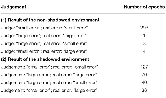
Table 5. Results of evaluation of the method using mileage and distance between positioning points.

The average positioning error of fixed elevation mask (15°) was 5.78 m, and that of variable elevation mask was 5.50 m. This result shows that when the elevation mask was adjusted according to the judgment result, the average positioning error was improved by approximately 0.3 m compared to when the elevation mask was always set to the same value of 15°. By applying this method, the positioning accuracy was improved for 59.5% of the epoch. The loss of six of 273 epochs can be prevented compared to when the elevation mask was always set to 15°. In the non-shadowed environment, the error size was successfully discriminated by the method, and the discrimination was very high at 97.6%. However, in the shadowed environment, the discrimination was at 72.1%. In this environment, the judgment's success rate decreased because the parts discriminated against as “small error” and as “large error” were mixed. However, as a result of setting the elevation mask using this judgment result, we confirmed that the positioning accuracy was improved, albeit with a small value of 0.3 m. The positioning accuracy did not improve much because only a few epochs can significantly improve 1 m or more when the 15° and 30° elevation masks were applied. Therefore, we believe that a great effect can be expected in an environment where the positioning accuracy can be greatly improved by adjusting the elevation mask. Moreover, distinguishing between regions where positioning is stable and where it is unstable is possible. Hence, this method can be used to construct an error map.

The estimation error method could be used to estimate the positioning error. However, a precise error amount cannot be obtained; therefore, we need to select a service that can use this method. We also confirmed that the method using mileage and distance between positioning points could be used for the magnitude of error judgment, especially in the non-shadowed environment, and displays a high error judgment rate. On the contrary, the judgment accuracy in the shadowed environment was lower. We evaluated the effect of changing the elevation masks using the result. Consequently, we confirmed that the error can be improved, albeit insignificantly.

7. Possible Error Map Applications

We discuss the possibility of the error map application in this section.

7.1. A-GPS

Assisted GPS (A-GPS) is a technology that uses information from base stations for positioning with mobile phones. A-GPS is useful for roughly grasping the user position from the received signal base station and narrowing down the user position. A technology called place engine performs positioning using Wi-Fi access points, even in indoor positioning, where satellite signals cannot be received. Therefore, in a shadowed environment, the positioning accuracy can be expected to improve by installation (e.g., beacons). For this purpose, a database of location information must be developed as an infrastructure. An error map can be used as a guide for setting up such infrastructure.

7.2. Elevation Mask Adjustment

We discussed this technique in the previous section. Satellites with low elevation angles generally often transmit low-quality signals. A receiver usually has a function that eliminates satellites transmitting low-quality signals by referring to the elevation angle. If the error map is used to estimate the “small error,” the result is used to apply a weak elevation mask. Consequently, the overall accuracy of the positioning could be increased.

7.3. RTK

RTK is one of the technologies that has been drawing attention in recent years. It is a method of obtaining a mobile station's coordinates by finding the relative position with the mobile station on the user side by employing a reference station whose coordinates are known. The method accuracy is said to be of the order of a few centimeters, and high positioning accuracy can be achieved. The RTK system is required to count the number of satellite carrier waves at the user receiver. However, they may be interrupted by blocking the signal at a shadow, such as a building. Consequently, positioning may not be stable, even if the RTK is used in a shadowed environment. The degradation of the RTK positioning accuracy can be prevented by eliminating a satellite with a low-quality signal. It is possible to determine whether the environment is shadowed or not by using an error map; thus, it is possible to improve the positioning accuracy by using the variable elevation mask described to eliminate satellites that may cause signal interruptions.

7.4. Dynamic Map

Current positioning systems often use sensors to perform highly accurate positioning. Positioning support using dynamic maps for transportation is expected as a support method. Technologies that use map information, such as map matching, are often used. A system that supports each user's positioning should be put to practical use by employing the map information and the 3D building information, and smartphone and automobile information as big data. In this study, we examined the method for making a GNSS positioning error map as part of such a dynamic map. Furthermore, using 5G is expected to increase the communication speed, reduce the hardware size of IoT systems, and improve the data mining technology to enable an efficient use of big data. We expect the availability of dynamic maps in the future.

8. Conclusion

In this paper, we mentioned a cognitive navigation system inspired by the CogInfoCom that extends human cognitive capabilities and would even enable life support. Also, we described details of the error map as the technical basis of a cognitive navigation system.

An error map was designed to display the accuracy of the positioning of GNSS. We mentioned the method to measure the positioning error of GNSS by using two GNSS receivers. We designed the technique in two ways using two GNSS receivers, namely the estimation of error using two GNSS receivers and the comparison of the error size assisted by the error map. First, we explained the problems related to positioning using GNSS and proposed the new error map idea to adopt the multi-path environment and acquire a better position result. Next, we investigated the positioning error caused by the multi-path under a shadowed environment when moving and stopping. Consequently, we confirmed that the distance of the two GNSS receivers and the average positioning error from these two receivers positively correlate. We proposed the two following methods according to the results: (1) error estimation by the linear regression; and (2) comparison of the error size assisted by the error map. We then evaluated the performance of the proposed method.

It is difficult to estimate the level of positioning error of GNSS. Usually, the number of satellites or Dilution of Precision (DOP) is used for that purpose. However, such methods cannot estimate the level of the error caused by multipath by buildings. A new idea to estimate the level of positioning error of GNSS is required by reflecting real filed positioning data. The proposed idea provides a useful and straightforward method to estimate the level of positioning error of GNSS by using a known distance of two GNSS receives.

Our method satisfied the target (error ≦ 1 m) of 20% of test data, but could not satisfy the target we set in sections 4 and 5. However, we can use our method for LBS, which does not require a critical boundary of accuracy. For the error size comparison, the no-shadow case provided an accuracy of over 90%; however, the accuracy was lower than 72% in the shadow case. We can distinguish the positioning stability; thus, we can offer a service to provide information about the possible error by using the error map and develop LBSs by incorporating the location's possible error.

The development of a real error map requires further study. If we develop an error map, we should consider several things, including the useful number of error levels (such as 3 or 5 or 10) and the number of epochs for error calculation. Also, the idea of developing and maintaining the error map is required. One possibility is to attach GNSS receivers on buses, trucks, and taxis to collect the position data and errors. The map must be frequently updated after developing the error map. This map provides information about the error level, and the user can rely on it as information to support positioning (e.g., shadow mask application to obtain more accurate position data or understand the position data reliability).

We think that many fields can be extended usability and performance by using the idea of CogInfoCom. We would like to try to use the concept of CogInfoCom in the different research areas.

Data Availability Statement

The raw data supporting the conclusions of this article will be made available by the authors, without undue reservation.

Author Contributions

All authors listed have made a substantial, direct and intellectual contribution to the work, and approved it for publication.

Funding

The part of the research results was obtained from the commissioned research by the National Institute of Information and Communications Technology (NICT), JAPAN. Also, this research was supported by JSPS KAKENHI Grant Number JP17H02249, JP18K11849, and JP17H01731.

Conflict of Interest

The authors declare that the research was conducted in the absence of any commercial or financial relationships that could be construed as a potential conflict of interest.

References

Baranyi, P., and Csapo, A. (2012). Definition and synergies of cognitive infocommunications. Acta Polytech. Hung. 9, 67–83.
Baranyi, P., Csapo, A., and Sallai, G. (2015). Cognitive Infocommunications (CogInfoCom). Cham: Springer International.
Iwase, T., Suzuki, N., and Watanabe, Y. (2013). Estimation and exclusion of multipath range error for robust positioning. GPS Solut. 17, 53–62. doi: 10.1007/s10291-012-0260-1
Kitani, T., Hatano, H., Onishi, H., and Hirao, S. (2012). A Method to Improve Positioning Accuracy of GPS by Sharing Error Information Among Neighbor Devices. Information Processing Society of Japan SIG Technical Report in Japanese 2012-ITS-49, 1–6.
Klobuchar, J. A. (1987). Ionospheric time-delay algorithm for single frequency GPS users. IEEE Trans. Aerospace Electr. Syst. 23, 325–331. doi: 10.1109/TAES.1987.310829
Kubo, N., Kobayashi, K., Hsu, L.-T., and Amai, O. (2017). Multipath mitigation technique under strong multipath environment using multiple antennas. J. Aeronaut. 49, 75–82.
Misra, P., and Enge, P. (2001). Global Positioning System Signals, Measurements, and Performance. Lincoln, MA: Ganga-Jamuna Press.
Miyata, H., Noguchi, T., Sakitani, A., and Egashira, S. (1996). Consideration on high accurate positioning with simplified DGPS. ITE Tech. Rep. (in Japanese) 20, 71–76.
Miyata, H., and Sakitani, A. (1997). Improving accuracy of simplified dgps positioning by the after processing. ITE Tech. Rep. (in Japanese) 21, 19–22.
Nakamura, Y. (2018). A research on reduction method of positioning error based on error characteristics under the same combination of gnss satellites. Utsunomiya: Utsunomiya University Graduation thesis (in Japanese).
Odaka, Y., Takano, S., In, Y., Higuchi, M., and Murakami, H. (2011). “The evaluation of the error characteristics of multiple GPS terminals,” in Proceedings of the 2nd International Conference on Circuits, Systems, Control, Signals (CSCS '11) (Prague), 13–21.
Osechas, O., Kim, K. J., Parsons, K., and Sahinoglu, Z. (2015). “Detecting multipath errors in terrestrial GNSS applications,” in Proceedings of the 2015 International Technical Meeting of The Institute of Navigation (Dana Point, CA), 465–474.
Rohani, M., Gingras, D., and Gruyer, D. (2016). A novel approach for improved vehicular positioning using cooperative map matching and dynamic base station DGPS concept. IEEE Trans. Intell. Transport. Syst. 17, 230–239. doi: 10.1109/TITS.2015.2465141
Saastamoinen, J. (1973a). Contributions to the theory of atmospheric refraction. Bull. Geodesique 30, 279–298.
Saastamoinen, J. (1973b). Contributions to the theory of atmospheric refraction. Bull. Geodesique 30, 383–397.
Saastamoinen, J. (1973c). Contributions to the theory of atmospheric refraction. Bull. Geodesique 30, 13–34.
Satirapod, C., and Chalermwattanachai, P. (2005). Impact of different tropospheric models on gps baseline accuracy: case study in Thailand. J. Glob. Posit. Syst. 4, 36–40. doi: 10.5081/jgps.4.1.36
Vincenty, T. (2013) (1975 (Published online: 2013)). Direct and inverse solutions of geodesics on the ellipsoid with application of nested equations. Surv. Rev. XXIII, 88–93. doi: 10.1179/sre.1975.23.176.88.
Keywords: Global Navigation Satellite System, error map, cooperative positioning, intelligent transport system, CogInfoCom
Citation: Ito A, Nakamura Y, Hiramatsu Y, Kitani T and Hatano H (2021) Developing an Error Map for Cognitive Navigation System. Front. Comput. Sci. 3:661904. doi: 10.3389/fcomp.2021.661904
Received: 31 January 2021; Accepted: 21 March 2021;
Published: 04 May 2021.
Edited by:
Péter Baranyi, Széchenyi István University, HungaryReviewed by:
Jozsef Katona, University of Dunaújváros, HungaryGyörgy Molnár, Budapest University of Technology and Economics, Hungary
Copyright © 2021 Ito, Nakamura, Hiramatsu, Kitani and Hatano. This is an open-access article distributed under the terms of the Creative Commons Attribution License (CC BY). The use, distribution or reproduction in other forums is permitted, provided the original author(s) and the copyright owner(s) are credited and that the original publication in this journal is cited, in accordance with accepted academic practice. No use, distribution or reproduction is permitted which does not comply with these terms.
*Correspondence: Atsushi Ito, atc.00s@g.chuo-u.ac.jp
†Present address: Yosuke Nakamura, OKI Software Co., Ltd., Saitama, Japan