Combining Dynamical and Statistical Modeling to Improve the Prediction of Surface Air Temperatures 2 Months in Advance: A Hybrid Approach
 Pascal Oettli1*
  Masami Nonaka1
  Ingo Richter1 Hiroyuki Koshiba2 Yosuke Tokiya2 Itsumi Hoshino2 Swadhin K. Behera1
- 1Application Laboratory Research Institute for Value-Added-Information Generation (APL VAiG), Japan Agency for Marine-Earth Science and Technology (JAMSTEC), Yokohama, Japan
- 2JERA Co., Inc., Tokyo, Japan
A new type of hybrid prediction system (HPS) of the land surface air temperature (SAT) is described and its skill evaluated for one particular application. This approach utilizes sea-surface temperatures (SST) forecast by a dynamical prediction system, SINTEX-F2, to provide predictors of the SAT to a statistical modeling system consisting of a set of nine different machine learning algorithms. The statistical component is aimed to restore teleconnections between SST and SAT, particularly in the mid-latitudes, which are generally not captured well in the dynamical prediction system. The HPS is used to predict the SAT in the central region of Japan around Tokyo (Kantō) as a case study. Results show that at 2-month lead the hybrid model outperforms both persistence and the SINTEX-F2 prediction of SAT. This is also true when prediction skill is assessed for each calendar month separately. Despite the model's strong performance, there are also some limitations. The limited sample size makes it more difficult to calibrate the statistical model and to reliably evaluate its skill.
Introduction
For the last two decades, seasonal climate prediction (SCP) has become an area of study in its own right (Pepler et al., 2015), similar to weather prediction and climate change projection. Continuous improvements (Doblas-Reyes et al., 2013) have increased the value of SCP in decision-making, though quantifying its benefits remains a challenge (Kumar, 2010; Soares et al., 2018).
In the agricultural sector, decision-making that adapts to climate variability is essential for food security (Hansen, 2002; Meza et al., 2008). For example, in Europe, SCP are helpful in the selection of winter wheat and planning of agro-management practices (Ceglar and Toreti, 2021). In the energy sector, the sudden weather changes and climate variability impact energy consumption (Auffhammer and Mansur, 2014) and, for example, the use of air conditioners (Auffhammer and Aroonruengsawat, 2012; Auffhammer, 2014).
SCP is also used in risk management (Troccoli et al., 2008) and crop insurance (Osgood et al., 2008; Carriquiry and Osgood, 2012), and is viewed as a viable alternative to traditional crop insurance in countries with rainfed agriculture (Leblois and Quirion, 2013), although its full adoption to the benefit of local farmers has still been slow so far (Leblois and Quirion, 2013). Also, combining dynamical and statistical modeling often increases the value of SCP information for decision makers and end-users, as it improves the skill of the forecast and can serve to downscale forecasts to relevant spatial scales. For example, working on the improvement of the Australian seasonal rainfall, Schepen et al. (2012) have confirmed that merging statistical and dynamical forecasts maximizes spatial and temporal coverage of skillfulness. This in turn enhances the value for end-users. However, Darbyshire et al. (2020) concluded that the practical value of SCP is still relatively low and inconsistent for seven Australian case studies and call for improvement of forecasts, in accordance with similar findings by Gunasekera (2018) in the energy sector, stressing the need to create more skillful seasonal forecasts. There are different ways to achieve improvements, like increasing the spatio-temporal resolution of seasonal forecast systems, correcting/adjusting the systematic errors (or bias) of such a system by downscaling or by constructing a statistical model linking a predictand and its predictors.
Oceans are major drivers of the climate system (Shukla, 1998) and the main source of seasonal predictability (Barnston, 1994 and references therein; Goddard et al., 2001; Shukla and Kinter, 2006) for temperature and precipitation. While dynamical prediction systems can accurately predict seasonal climate in the tropics due to the strong coupling between ocean and atmosphere, prediction skills of the SAT are limited in many terrestrial parts of the world (Figure 1), partly because dynamical forecast systems cannot fully reproduce the relevant atmospheric processes (Shukla, 1985; Branković et al., 1990; Livezey, 1990; Milton, 1990; Barnston, 1994; Sheffield et al., 2013a,b; Henderson et al., 2017). Also, many of the teleconnections between the tropics/sub-tropics and the mid-latitudes are not well-represented, with the exception of those arising from the El Niño–Southern Oscillation (ENSO). As monthly-scale SAT in the extra-tropics, including our target region, can be strongly affected by atmospheric teleconnections (e.g., Oettli et al., 2021), there is a potential gain in skill that could be realized by representing teleconnections between the tropics and the mid-latitudes through statistical modeling, by using sea-surface temperature (SST) as a predictor of the surface air temperature (SAT).
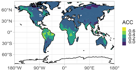
Figure 1. Anomaly correlation coefficient between the 2-month lead SINTEX-F2 ensemble mean 2-meter temperature and the GHCN CAMS 2-meter temperature (Fan and van den Dool, 2008) for the period 1983–2015 (396 months).
The conventional approach involves multivariate linear statistical models (Barnston, 1994; Drosdowsky and Chambers, 2001). While these models are easy to construct, they are rather limited because they miss some of the important non-linear links between SST and SAT. Machine learning (ML), a subset of artificial intelligence that improves algorithms automatically through experience (Mitchell, 1997; Hastie et al., 2009; James et al., 2013; Kuhn and Johnson, 2016), can capture such non-linearities through statistical modeling.
Artificial Neural Networks (ANN) and Support Vector Machines (SVM) have been successfully used to forecast SAT at different time scales (Cifuentes et al., 2020; Tran et al., 2021). The predictability comes from the temperatures only (e.g., Ustaoglu et al., 2008; Chattopadhyay et al., 2011), or in association with other atmospheric variables (e.g., Mori and Kanaoka, 2007; Smith et al., 2009), oceanic modes (Salcedo-Sanz et al., 2016), or SST indices (Ratnam et al., 2021b). But the skills of such forecast systems are highly variable (Cifuentes et al., 2020) and dependent on past observations. Could the skill of such models be improved by including oceanic conditions forecast by a dynamical model?
In the present study, we attempt to harness the skills from both dynamical and statistical modeling approaches by adopting a hybrid approach to SCP, which has been demonstrated to yield skillful seasonal precipitation forecasts in northwest America (Gibson et al., 2021). In this approach, a dynamical prediction system, SINTEX-F2 (Doi et al., 2016, 2017), is used to provide the SST anomaly field, from which potential predictors of the SAT are extracted. The extracted predictors are used to construct a statistical prediction model using the following nine ML algorithms: Artificial Neural Networks with single- (SLP) and multi-layer perceptrons (MLP); Support Vector Machines with linear (SVML) and radial kernels (SVMR); Random Forests (RF); relatively recent approaches based on the gradient boosting of decision trees, namely the extreme gradient boosting with linear (XGBL) and tree-based (XGBT) approaches, and CatBoost (CBST); and Bayesian additive regression trees (BART). These boosting techniques are largely used in classification problems (Hancock and Khoshgoftaar, 2020; Ibrahim et al., 2020; Xia et al., 2020; Zhang et al., 2020; Jabeur et al., 2021; Luo et al., 2021), but less so for regression problems. This study provides a good opportunity to evaluate the skills of boosting procedures in the prediction of SAT.
In this study, we focus on SAT because it is a crucial climatic factor in agriculture (because it conditions the crop growth and its physiology) and in the energy sector (because it has a large impact on the fuel consumption for heating and cooling systems), two give two examples. Thus, the seasonal prediction of SAT may help to mitigate impacts of climate variations by allowing to take appropriate action in advance.
Motivated by an ongoing project in the energy sector, the target lead time for our hybrid model is 2 months. Forecasts between monthly and seasonal time steps are important for mid-term planification, such as the water and energy management (Oludhe et al., 2013) or the indoor residual spraying for malaria transmission control and elimination (World Health Organization, 2015). Therefore, we use the 2-month lead SST forecasts from the dynamical model as input for the hybrid prediction system (HPS). Details of the HPS and associated data are presented in Section Materials and Methods, and then the hybrid system skills are assessed in Section Application to the Kantō Region, using the Kantō region (a geographical area of the main island of Japan, comprising the Kantō plain to the central eastern part and mountainous region to the North and the West; Figure 2A), as an example of application. Finally, results are discussed in Section Summary and Discussion.
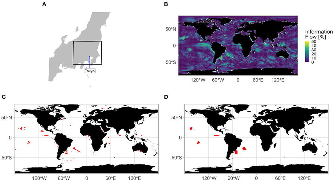
Figure 2. (A) Location of the Kantō region (black box) in Japan. (B) Example of normalized information flow calculation, (C) grid points complying with the selection criterion (NIF ≥ 30%) for the global region, and (D) areas complying with the selection criteria (NIF ≥ 30%, surface area ≥ 300,000 km2) for the global region.
Materials and Methods
SINTEX-F2 Seasonal Prediction System
The SINTEX-F2 prediction model (Doi et al., 2016), and its upgraded version, the SINTEX-F2 3DVAR system (Doi et al., 2017) forecast monthly mean SST at various lead times.
Our goal is the prediction of the SAT anomaly in the Kantō region, 2 months in advance using the information coming from the SINTEX-F2 SST anomaly prediction fields. To achieve this purpose, the predicted SST anomalies at 2 months lead time are taken for all 24 members plus the ensemble mean (hereafter 2mlEMs). The monthly anomalies we use are calculated by subtracting the 1983–2015 monthly climatology and removing the linear trend calculated over the same time period.
The SINTEX-F2 prediction model has high skill in the prediction of the ENSO (Luo et al., 2005, 2008b; Jin et al., 2008; Doi et al., 2016), a fundamental requirement for any seasonal prediction system (Stockdale et al., 2011) to be considered skillful. SINTEX-F2 is also successful in predicting the Indian Ocean Dipole (Luo et al., 2007, 2008a; Doi et al., 2016) and the subtropical dipole modes (Yuan et al., 2014).
Surface Air Temperatures in the Kantō Region
From the Automated Meteorological Data Acquisition System (AMeDAS) network maintained by the Japanese Meteorological Agency (2018), monthly mean SAT from 102 stations are extracted to cover the Kantō region (138–141°E, 35–37°N, Figure 2A), for the period March 1983 (due to the 2 months difference)–July 2020. Except for the initial quality check performed at JMA, no further quality check or homogenization has been performed before the analyses. An SAT index for the Kantō region is calculated by arithmetically averaging the values of the 102 stations, without weighting by latitude, considering the rather small region used in this study. To comply with SINTEX-F2 forecasts, departures from the 1983 to 2015 monthly climatology are calculated, and the linear trend calculated over the same period is subsequently removed.
Cause-and-Effect Relationships
The natural way to find linear relationships between time series is the calculation of the correlation coefficient. Correlation, however, does not imply causation (Barnard, 1986) and is not sufficient to establish causality (Sugihara et al., 2012). Therefore, different statistical concepts have been developed to identify the mutual information (Shannon, 1948) between time series and the underlying cause-and-effect relationships between them. Popular statistical concepts include the Granger causality (Granger, 1969), the transfer entropy (Schreiber, 2000), the climate networks (Tsonis and Roebber, 2004), the convergent cross mapping (Sugihara et al., 2012), or the information flow (Liang and Kleeman, 2007a,b; Liang, 2008, 2014, 2016).
The information flow (IF) measures the rate of information flowing from X2 to X1 and the maximum likelihood estimator of the rate of IF (Liang, 2014) is:
with Cij the sample covariance between Xi and Xj, and Ci, dj the sample covariance between Xi and a series derived from Xj using the Euler forward differencing scheme: , with k = 1 or k = 2, some integer defining the time lag of the Euler forward scheme (i, j = 1, 2), n∈N (the sample size), and Δt the time step (Liang, 2014, 2019).
The IF has been shown to be efficient for detecting causality in linear and non-linear systems (Stips et al., 2016). In order to assess the relative importance of an identified causality, a normalized version of the information flow (NIF) has been developed (Liang, 2015; Bai et al., 2018), as:
with abs(T2 → 1) the absolute IF and the rate of change of the stochastic effects, defined as (adapted from Bai et al., 2018):
with E the mathematical expectation, g11 the perturbation amplitudes of X1 and ρ1 the marginal probability density function of X1 (Liang, 2019).
The normalization avoids the relative causality to become too small (Bai et al., 2018).
Design of the Hybrid Prediction System
Since the model should be evaluated against a data set independent of the one used to train the prediction system (Davis, 1976; Chelton, 1983; Dijkstra et al., 2019), the available data are divided into three subsets. The calibration subset covers the period March 1983 to February 2010 (for a total of 27 years), the validation subset covers the period March 2010 to February 2020 (10 years), and the evaluation subset covers March 2020 to August 2021 (1 year). While it not possible to calculate skill metrics on the evaluation subset, we consider it is a good way to see whether a totally independent subset (i.e., not used either during the training step or during the optimization step) is able to reproduce observed anomalies for different seasons. All subsets start from March because of the 2 months lead initialization of SINTEX-F2.
Defining the Potential Predictors
For each month, the NIF is used to quantify the flow of information from each grid point of each of the 25 SINTEX-F2 2mlEMs into any SAT time series of interest (see Figure 2B for an illustration with the SAT index of the Kantō region) and delineate areas of interest as potential sources of predictability, and thus as potential predictors to use in our hybrid prediction model (upper part of Figure 3). For each 2mlEMs, only grid points with an NIF significant at 99% (Liang, 2015) are kept, reducing the amount of data. Subsequently, grid points with an NIF larger or equal to 30% are kept as a first group of potential predictors (Figures 2C, 3, “GR-Z” block). A second class is then defined by aggregating adjacent retained grid points and calculating the convex hull (i.e., the smallest convex area containing them; Figure 2D), in order to determine regions that potentially offer predictability. Only areas with a surface area larger or equal to 300,000 km2 are kept in the second group (Figure 3, “GR-Z” block). The extraction is done globally (Figure 3, “GR-Z” block), but also for the tropical region only (30°N−30°S), where the SINTEX-F2 has high skill (Doi et al., 2016).

Figure 3. Workflow of the hybrid prediction system (HPS). For each month, the general process consists of NIF calculation, followed, in order, by the selection of geographical region and zones (GR-Z), the selection of predictors (PredS), the calibration of models through different machine learning algorithms (Alg), and the optimal configuration (OC) ending to the creation of HPS. SLP and MLP are artificial neural network with single- and multi-layer perceptron, respectively; SMVL and SVMR are the support vector machine with linear and radial kernels, respectively; RF is the random forest; XGBL and XGBT are extreme gradient boosting with linear and tree-based approaches, respectively; CBST is CatBoost and BART is Bayesian additive regression trees.
Selecting the Predictors
A set of predictors is designed by performing a feature selection (Figure 3, “PredS” block). First, we test for multicollinearity to reduce the redundancy contained in the pool of potential predictors. The absolute values of pair-wise correlations are considered. If two variables have a high correlation, the function looks at the mean absolute correlation of each of the two variables with all the other variables and removes the variable with the largest mean absolute correlation. The cutoff is fixed at 0.8.
Second, the feature selection itself is performed by using the Boruta method (Kursa and Rudnicki, 2010; Kursa et al., 2010), which iteratively compares the importance of attributes with their shuffled versions of the original attribute (i.e., their “shadows”). At each iteration, the importance of original attributes is compared to their respective “shadow” versions. All original attributes that have smaller importance than the “shadow” are dropped. Shadows are re-created in each iteration. For this study, we fixed the maximum number of iterations at 10,000. A Random Forest algorithm (Breiman, 2001) is used to provide the variable importance measure necessary for the Boruta method to achieve the selection.
Finally, the variance inflation factor (VIF; Marquardt, 1970; Fox and Monette, 1992) is calculated for the remaining predictors and those with values larger or equal to 5 are kept, to create the final selection of predictors. All the three steps of the feature selection are performed over the calibration period and for the two classes of predictors previously defined (i.e., grid points and convex hull areas).
A second set of predictors (Figure 3, “PredS” block), including all the potential predictors without the prior selection, is also defined. Here, the idea is to let the machine learning (ML) algorithms manage the whole data and create an optimal model.
Performance Measurement
The accuracy of the predictions is assessed by calculating several metrics between the observations and the predictions.
• Anomaly Correlation Coefficient (ACC): While the ACC is sensitive to outliers, it remains a simple metric to evaluate the co-variability of two time series. A positive value (as close as possible to +1) indicates similar variability and is targeted;
• Root Mean Square Error (RMSE): A popular measurement of prediction model accuracy. RMSE should be as small as possible (with a perfect model, RMSE would be equal to 0);
• Mean Absolute Error (MAE; Willmott and Matsuura, 2005): Another measurement of model error;
• Mean Absolute Scaled Error (MASE; Hyndman and Koehler, 2006): Calculated by scaling the error based on the in-sample MAE from the random walk forecast method. MASE is below 1 when the forecast is better than the average one-step naïve forecast. MASE has been shown (Franses, 2016) to be consistent with the standard statistical procedures for testing equal forecast accuracy (Diebold and Mariano, 1995);
• Linear Error in Probability Space (LEPS; Ward and Folland, 1991): Provides an equitable scoring system, but can tend to assign better score to poorer forecasts near the extremes (“bend back”). It is a negatively oriented score, where 0 is a perfect score;
• Skill Error: A positively oriented score that is considered an enhancement of the LEPS (Potts et al., 1996) because it solves the “bend back” problem. Because this score is not widely used, we show the SK together with the LEPS. SK is defined as
with f the predicted values, a the actual values, overbar the mean of all samples of the variable, n the total number of samples and e is the forecast error (i.e., a–f). In the MASE equation, the denominator is the mean absolute error of 1-month-ahead forecasts from each data point in the sample (Hyndman, 2006) i.e., ft = at−1, with T the training period and t a time step during T. In LEPS and SK equations, CDFa is the cumulative density function of actual values.
Outcomes of the hybrid approach are compared to the SAT index for the Kantō region calculated from the SINTEX-F2 ensemble mean (i.e., the arithmetic average of the 24 members). The 2-month persistence is also considered as a one-period-ahead naïve forecast (i.e., the SAT anomalies taken 2 months before are considered as good predictors of the SAT anomalies 2 months after). Hybrid prediction systems must have better performance than this naïve forecast to show skills in predicting SAT in the Kantō region.
Machine Learning
To predict an SAT index from 2mlEMs, we need to map the routes connecting SAT and SST, to create a general rule, i.e., a statistical model able to accurately predict the SAT from the 2mlEMs. ML can efficiently describe underlying processes between input and output data, mapping the paths from the former to the latter, and is thus applied to our purpose.
Tuning parameters (or hyperparameters) of the algorithm are generated by a random search (Bergstra and Bengio, 2012), which generates 10 combinations of them. The details of the tuning parameters for each method are introduced below.
Artificial Neural Network
The architecture of the artificial neural network (ANN) is designed to mimic the human brain and how the neurons interact with each other, how they are activated and how they learn. ANN consists of an input layer, one or multiple hidden layers and an output layer. A hidden layer is constructed by interconnecting artificial neurons (or nodes) with a specific weight and threshold (which determine whether a node is activated or not). ANNs are often used for pattern recognition but are increasingly used in a broad range of applications, including ENSO forecasts (Ham et al., 2019; Yan et al., 2020).
We use a simple feed-forward multi-layer perceptron with a single hidden layer (i.e., single-layer perceptron) for its ease of use and robustness. The tuning parameters consist of the number of artificial neurons of the hidden layer and the weight regularization (via an exponentially decay to zero), which both to helps the optimization process and avoids over-fitting (Venables and Ripley, 2002). The internal number of iterations to hit the local minima, i.e., the improvement of accuracy through training, is set at 100.
In addition, we also use a multi-layer perceptron with three hidden layers, instead of one, and threshold activation, to alter the results of the ANN. The tuning parameters are the number of nodes in each hidden layer.
Random Forest
A random forest fits a number of decision tree classifiers (which learn simple decision rules inferred from the data features) on various sub-samples of the dataset and uses averaging to improve the predictive accuracy and control over-fitting. The tuning parameter is the number of variables randomly sampled as candidates at each split. The number of trees to grow is set to 500, to ensure that every input row gets predicted at least a few times.
Support Vector Machine
Support vector machine minimizes the coefficients (instead of the squared error in the case of linear regression) in order to reach an acceptable error of the model. A choice of different kernel functions (i.e., a pattern analysis to identify recurrent relationship in datasets) can be specified for the decision function (i.e., decide the acceptable error). Expecting the results being sensitive to the use of different kernels, we choose linear and radial kernels. The former is the dot product between two given observations while the latter creates complex regions within the feature space. The tuning parameter for the linear kernel is the cost regularization parameter, C, which controls the smoothness of the fitted function. In addition to the C parameter, the tuning parameter s (the inverse kernel width) is available in radial kernels.
Gradient Boosting
Gradient boosting (Figure 3, “Alg” block) is an ensemble learning technique to build a strong classifier from several weak classifiers (typically decision trees), through iteration (Breiman et al., 1984; Friedman, 1999a,b). Here we used the XGBoost implementation (Chen and Guestrin, 2016), which gives better performance and a better control of over-fitting issues. Two types of boosters are utilized to create the prediction system, a linear model, with squared loss as objective function, and a tree-based model.
The maximum number of boosting iterations (trees to be grown) is common to both boosters. The linear model has two other hyperparameters: the L1 regularization (lasso regression which adds “absolute value of magnitude” of coefficient as a penalty term to the loss function) and the L2 regularization (ridge regression which adds “squared magnitude” of coefficient as a penalty term to the loss function). In the case of the tree-based model, the maximum depth of a tree, the learning rate (scaling the contribution of each tree, to prevent overfitting by making the boosting process more conservative), the minimum loss reduction (to make a further partition on a leaf node of the tree), subsample ratio of columns when constructing each tree, the minimum sum of instance weight (to stop further partitioning of the tree), and the subsample percentage (random collection of the data instances to grow trees and prevent overfitting).
The CatBoost implementation (Dorogush et al., 2018; Prokhorenkova et al., 2019), a more recent gradient boosting of decision trees, is also used. It provides a different kind of boosting through a symmetric procedure. This approach imposes that all nodes at the same level test the same predictor with the same condition, allowing for a simple fitting scheme and efficiency on CPUs. Also, to avoid overfitting, the optimal solution is found by the regularization operated by the tree structure itself. In this algorithm, the number of trees, the depth of trees, the learning rate, the coefficient of the L2 regularization, the percentage of features to use at each iteration and the number of splits for numerical features are the tuning parameters.
Bayesian Additive Regression Trees
Inspired by the boosting approach i.e., summing the contribution of sequential weak learners to build a strong learner, Bayesian Additive Regression Trees (BART; Chipman et al., 2010) depends on an underlying Bayesian probability model (Figure 3, “Alg” block). The bartMachine implementation (Kapelner and Bleich, 2016) is used in our prediction framework.
The associated hyperparameters are the number of trees to be grown in the sum-of-trees model, the prior probability that E(Y |X) is contained in the interval (ymin, ymax) based on a normal distribution, the base and power hyperparameters in tree prior probability for whether a node is non-terminal or not, and the degrees of freedom for the inverse χ2 prior.
Limitations
Machine learning approaches have recently gained large popularity in climate sciences (Monteleoni et al., 2013; Lakshmanan et al., 2015; Voyant et al., 2017; Chantry et al., 2021), but concerns and constraints still exist (Makridakis et al., 2018). First, it is hard to derive physical understanding through the use of ML, even though some attempts have been made to address this issue (McGovern et al., 2019). The computational complexity of the algorithms, particularly the most recent ones, and the need of lengthy batch training can be a limitation to the use of ML. Also, specially trained algorithms are still required to perform specific tasks. The risk of overfitting is also an important concern and must be kept in mind. Closely related, a balance between interpretability and accuracy must be found when using ML. Relationships between variables that do not exist in the training data are likely to be missed in an independent data set, creating a limitation in the use of ML. Finally, the length of the training data may be an issue, as small datasets may limit pattern recognition (Raudys and Jain, 1991; van der Ploeg et al., 2014).
Training Process
To address the issue of the small sample size of the calibration period, bootstrapping (Efron, 1979) is used during the calibration phase to estimate the extra-sample prediction error (Figure 3, “Alg” block). Bootstrapping involves the generation of random sampling with replacement to estimate the error. It also introduces a bias because the replacement introduces repetitions of the same observation. In order to reduce the bias, the 0.632 bootstrap estimator (Efron, 1983; Efron and Tibshirani, 1997) is used, because on average each bootstrap sample contains about two thirds of observations. The optimal regression model is selected as the one which minimizes the MASE, after intermediate models have been built by resampling the calibration datasets 500 times.
The validation subset is subsequently used to evaluate the performance of the model previously trained, as well as to construct optimized forecast systems. Finally, an evaluation subset is used to assess the skills of the HPS.
Optimizing the Time Series
For each month in our training data, nine (9) ML algorithms are used to construct prediction models from two (2) geographical regions (global and tropical), two (2) classes of zones (grid points and convex hull area), and two (2) sets of predictors (selection of features and all features). As a result, a total of seventy-two (72) prediction models (hereafter ML configurations) associating Geographical Region-Zone-Predictor Set-Algorithm (GR-Z-PredS-Alg) are constructed for the calibration period and evaluated over the validation period (Figure 3).
Using the same predictors, each prediction system can be viewed as an ensemble member with its own internal condition and uncertainties. The ensemble mean of the 72 prediction models is calculated by averaging the outcome, as it is usually, but not always, more skillful than using any of the 72 models individually (Fritsch et al., 2000; Hagedorn et al., 2005; Eade et al., 2014).
We also assume that an individual model can outperform all other models for a specific calendar month. Thus, from the monthly 72 ML configurations, an optimized prediction is also calculated, according to the monthly performance measured over the validation period (Figure 3, “OC” block). For each month, the ACC (hereafter ACC_crit) is calculated between the prediction of each model and the observed SAT anomalies, and the model with the largest positive ACC is kept. This is also done according to the smallest RMSE (hereafter RMSE_crit) and the smallest MASE (hereafter MASE_crit). As a result, three optimized predictions are constructed, one for each of those three methods.
Finally, the long-term and monthly linear trends based on the observed SAT index (1983–2015 period) are added back to the observed and forecasted SAT anomalies.
In the present prediction system, we introduce an original hybrid approach that combines dynamical and statistical (machine learning) methods, in a new way. The major characteristic of this hybrid system is that predictors for the statistical part are not taken from observation (with or without time lag), but are provided by the 2-month lead SST forecasts from the SINTEX-F2 seasonal prediction system. In this way the system benefits from the ability of the dynamical prediction system to predict SST anomalies 2 months in advance. The hybrid approach also aims at statistically inferring teleconnections between remote SST anomalies and mid-latitudes, which are generally misrepresented in the dynamical prediction system.
In the case study below, all calculations have been performed on a personal computer with 8 cores [Intel(R) Xeon(R) CPU E5-1620 v3 @ 3.50 GHz] using the R programming language (R Core Team, 2019) and packages “caret” (Kuhn, 2020), “neuralnet” (Fritsch et al., 2019), “randomForest” (Liaw and Wiener, 2002), “RSNNS” (Bergmeir and Benítez, 2012), “kernlab” (Karatzoglou et al., 2004), “catboost” (Dorogush et al., 2018), “bartMachine” (Kapelner and Bleich, 2016), and “xgboost” (Chen et al., 2020) and required about 120 h to complete.
Application to the Kantō Region
The Kantō region is a highly populated area (43 million in 2015; Ministry of Internal Affairs and Communications, 2020) with high energy demand, particularly during boreal summer and winter. In summer, the heatstroke death rate increases with higher temperature and humidity (Akihiko et al., 2014) in the Kantō region. Akihiko et al. (2014) suggest that early warning systems based on SCP can be developed to reduce the risk of heatstroke, by forecasting the probability of heatwave occurrence a few months in advance.
At the same time, a significant part of the electricity demand in the region is met by thermal power plants, requiring good planning for the fuel management and logistics sufficiently ahead of time. SCP could potentially help in the management of fuel and in the planning of the operation to reduce the cost of the operation. For example, the Northern Illinois University saved approximately $500,000 in natural gas purchase with the help of climate information and forecast tools developed by a faculty member and a group of undergraduate meteorology students (Changnon et al., 1999).
We apply our hybrid prediction system (Figure 3) to the Kantō region. To put it simply, for each month of the year, the NIF is first calculated between the 25 2mlEMs and the Kantō SAT index during the calibration period. Then predictors are extracted and used to construct the 72 GR-Z-PreS-Alg. Finally, monthly SAT anomalies for the Kantō region are calculated over the validation period, using the GR-Z-PreS-Alg applied on the information provided by the 2mlEMs.
Evaluation of the Training Stage
The performance of the 72 monthly models (GR-Z-PreS-Alg) is evaluated by the ACC and RMSE calculated during the resampling phase of the training stage, between observed and forecasted SAT anomalies (Figure 4). In terms of ACC, performances are very similar across calendar months, with most of the coefficients ranging between 0.25 and 0.90. Performances are more variable with RMSE, some trained models being less accurate in July and February with RMSE >1.0. But overall performances are similar between months.
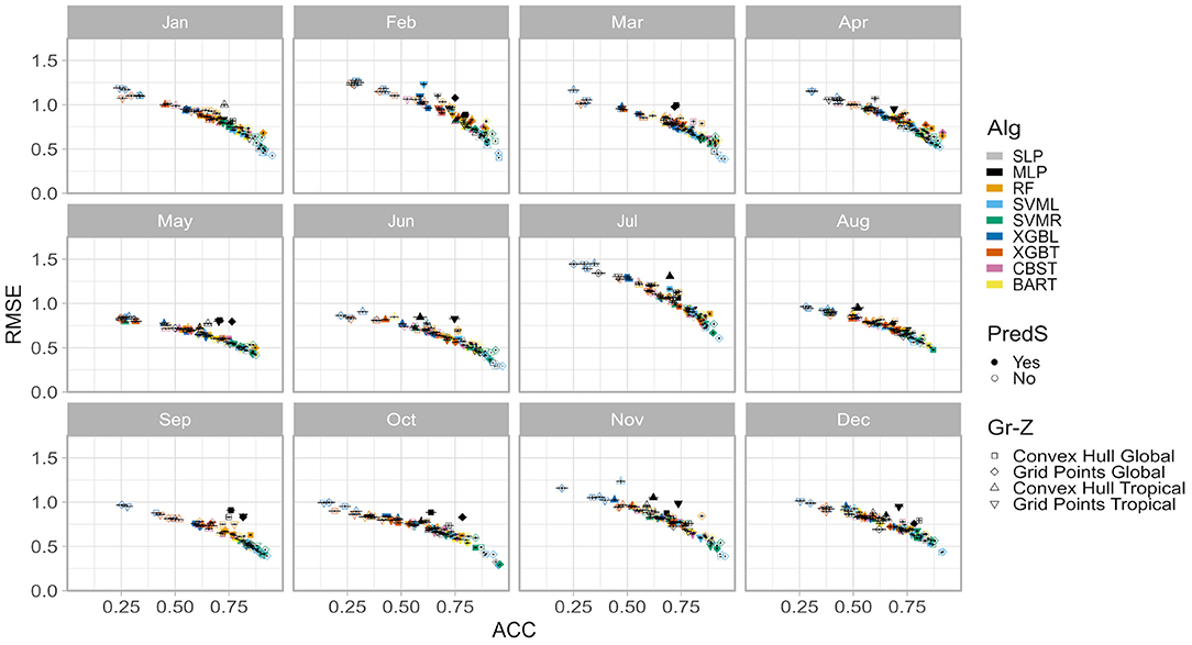
Figure 4. Comparison of model performances during the training phase, in terms of anomaly correlation coefficient (ACC) and root mean square error (RMSE). Shapes correspond to the different combination geographical region/zone (Gr-Z). Colors are the ML algorithms (Alg) with a filling (contour) corresponding to the existence (absence) of feature selection. Vertical and horizontal segment are the dispersion of the performance across the samples.
Across months, XGBL (dark blue) and XGBT (orange) without selection features (open symbol) appear to perform less well-compared to SVML (soft blue), SVMR (lime green), and SLP (gray) with feature selection (closed symbol). Other models are distributed between these two groups of models, following a curved line (better models have both lower RMSE and higher ACC). MLP (black) is a noticeable exception with most of the time high ACC associated to higher RMSE.
However, these results are biased because the evaluation of models is done against the data used to calibrate those models, with a high risk of overfitting, making them less generalizable. In order to possibly overcome this issue, forecasts from all the available monthly GR-Z-PreS-Alg are calculated and the monthly optimization of the time series is performed for the validation period.
Evaluation of the Optimizations
Over the validation period, monthly ACC are calculated between the output of each GR-Z-PreS-Alg and the observed SAT anomalies of the Kantō region (Figure 2A) over the validation period. It is clear from Figure 5 that some ML configurations performed better than others for the same month (some ACC are even negative). In January, the optimal GR-Z-PreS-Alg is the CaBoost (CBST) using all the selected areas of the global region (dark blue bar in the Jan/CBST panel, “Yes” line) with an ACC of 0.50. Other monthly optimal ML configurations can be found in Table 1. Interestingly, all ACC values are around 0.70 or above, ranging between 0.68 (in March) and 0.93 (in July), with the exception of January, February, and November in which a much smaller accuracy (ACC = 0.50, 0.44, and 0.48, respectively) of the optimal choice is obtained, implying that the hybrid model is struggling to accurately predict the SAT anomalies during these months. Another interesting result is the difference between the ACC of models calculated with the calibration subset (Figure 4) and the ACC shown in Figure 5. Support vector machines have good skills during the calibration step, but have generally poor performances with the validation subset, with the exception of boreal summer (SVML is selected as the best approach in August; Table 1). By contrast, gradient boosting approaches were not performing well with the bootstrapping validation, but are more skillful with the validation subset (XGBL/T are selected 6 months out of 12). Results also confirm that the search for an optimal GR-Z-PreS-Alg for each month is a useful approach.
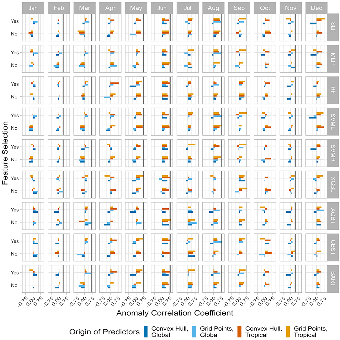
Figure 5. Monthly anomaly correlation coefficients (ACC) between the observed SAT index anomalies in the Kantō region and the forecasted SAT index anomalies during the validation period (March 2010 to February 2020). Each row is the results for a machine learning (ML) algorithm for each month (column). “SLP” is the single-layer artificial neural network, “MLP” is the multi-layer (3 layers) version, “RF” is the random forest, “SVML” is the support vector machine with a linear kernel, “SVMR” is the version with a radial kernel, “BART” is the bartMachine implementation of the BART algorithm, “XGBL” is the linear XGBoost implementation of the gradient boosting and “XGBT” is the tree-based XGBoost implementation. ML are run with the selected predictors (“Yes”) or with all the predictors (“No”). The origin of the predictors is provided by the colors. Vertical black lines denote the best coefficient my month.

Table 1. Optimal selection of monthly GR-Z-PredsS-Alg based on anomaly correlation coefficient criterion (ACC_crit).
We test an alternative approach for finding optimal configurations. In this approach, we use the RMSE_crit, rather than the ACC_crit, as our skill metric (Figure 6). For example, in January, the optimal combination is the linear gradient boosting using all the predictors (convex hull areas) of the global region (RMSE = 0.9164; dark blue bar in the Jan/XGBL panel, “No” line). Other combinations are summarized in Table 2. With this approach, March has the worst score (1.0952) while June has the best (0.4259). Similar to ACC_crit, SVML/R have poorer performances with the RMSE_crit compared to the calibration step, but are selected more often (three times). Again, XGB(L/T) are selected six times.
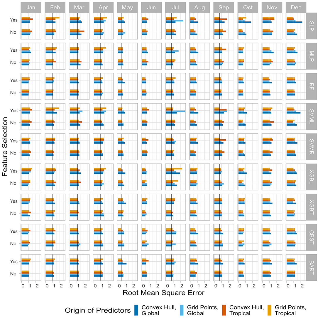
Figure 6. Same as Figure 5 but for the root mean square error (RMSE).
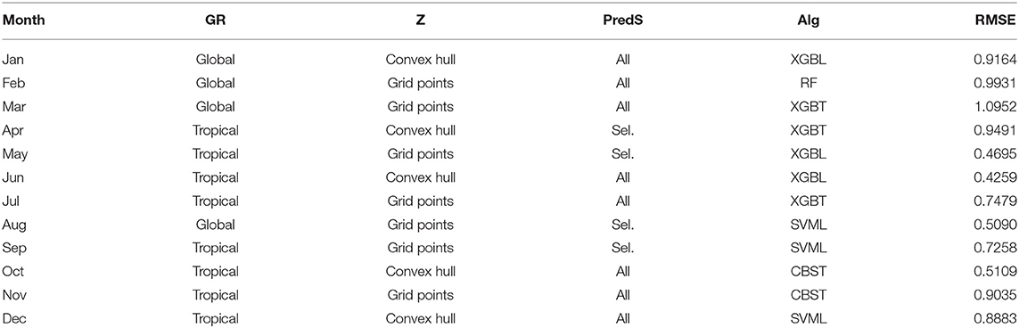
Table 2. Same as Table 1 but from the root mean square error criterion (RMSE_crit).
The same method of optimized selection is applied with the MASE_crit as selection metric (Figure 7) and the final optimal combination for each month is summarized in Table 3. It is worth noting that with this criterion, most of the models are based on extreme gradient boosting (XGBL/T; 6 models) and support vector machine (SVML/R; 5 models). The exception is April with the single-layer artificial neural network.
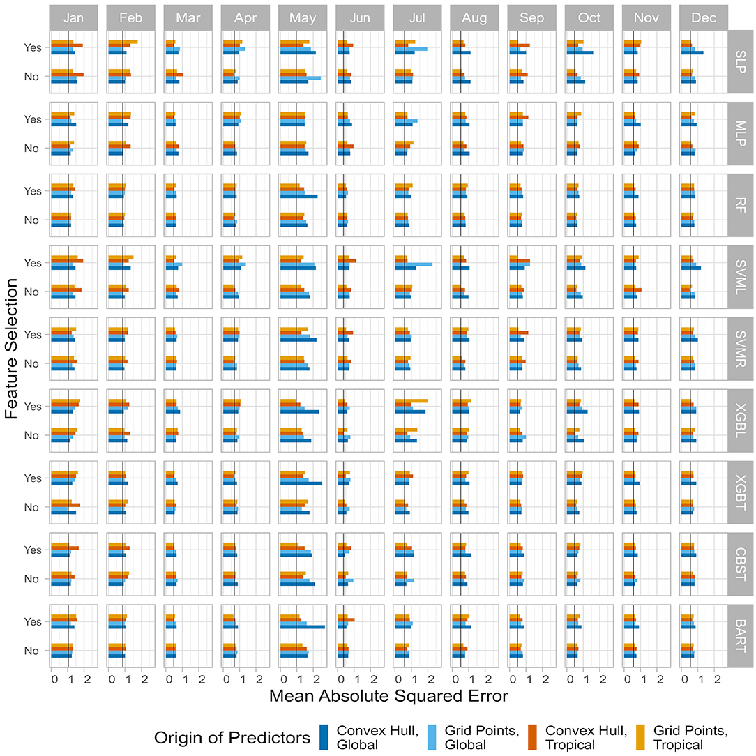
Figure 7. Same as Figure 5 but for the mean absolute scaled error (MASE).

Table 3. Same as Table 1 but from the mean absolute scaled error criterion (MASE_crit).
Together with the ensemble mean (Figure 8A; orange line), three optimized predictions of SAT index anomalies in the Kantō region are constructed, respectively, from the ACC_crit (bright yellow line), RMSE_crit (soft blue line), and MASE_crit (dark blue line). The observed SAT index is also shown for comparison (Figure 8A; black line). Overall interannual variability appears to be quite well-predicted by the various simulated SAT indices. In 2015–2016 or in 2018–2019, models are able to capture the seasonal variability. But sometimes, like in 2012–2013 or 2017 for example, all models have difficulties to capture correct values of SAT, particularly in boreal winter. The three optimized systems have anomaly correlation coefficients larger than 0.5 (Figure 9A), which is better than that of the SINTEX-F2 ensemble mean and the persistence (r < 0.2). Based on other accuracy metrics, the three optimized hybrid systems also systematically outperform the SINTEX-F2 ensemble mean and the 2-month lead persistence with smaller RMSE, MASE, MAE, and LEPS, and larger SK (Figure 9A).
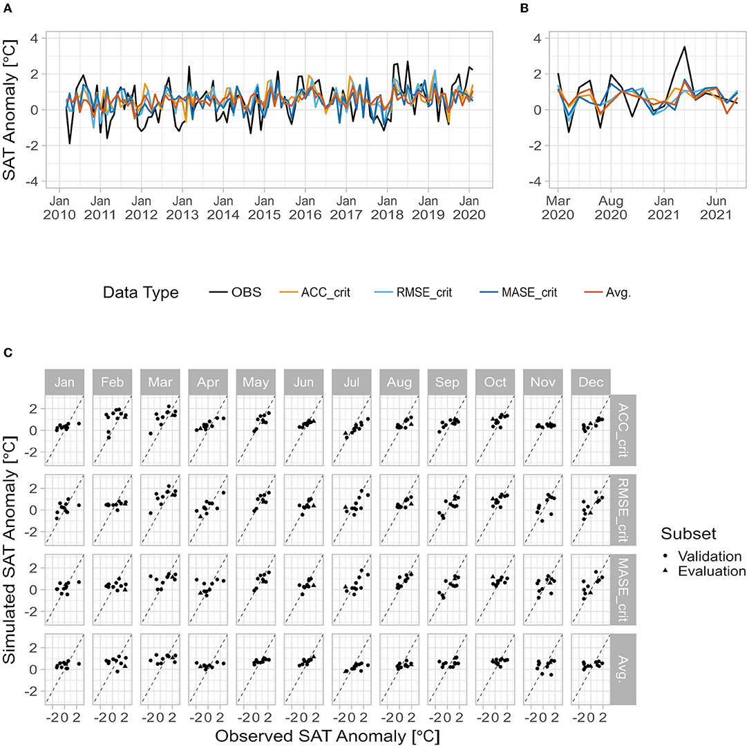
Figure 8. (A) Observed (black line) and predicted SAT index anomalies in the Kantō region for the validation period. Time series of the prediction consist of the average of the models (orange line) and optimized time series according to the anomaly correlation coefficient (yellow line), the root mean square error (cyan line) and the mean absolute scaled error (blue line). Long-term and monthly linear trends are restored. (B) Same as (A) but for the evaluation period. (C) Monthly stratification of scatter plots of the observed anomalies (x-axis) vs. the predicted anomalies (y-axis). Black dots are the forecasts for the validation period and black triangles for the evaluation period. Rows correspond to the different types of prediction system and columns to the month.
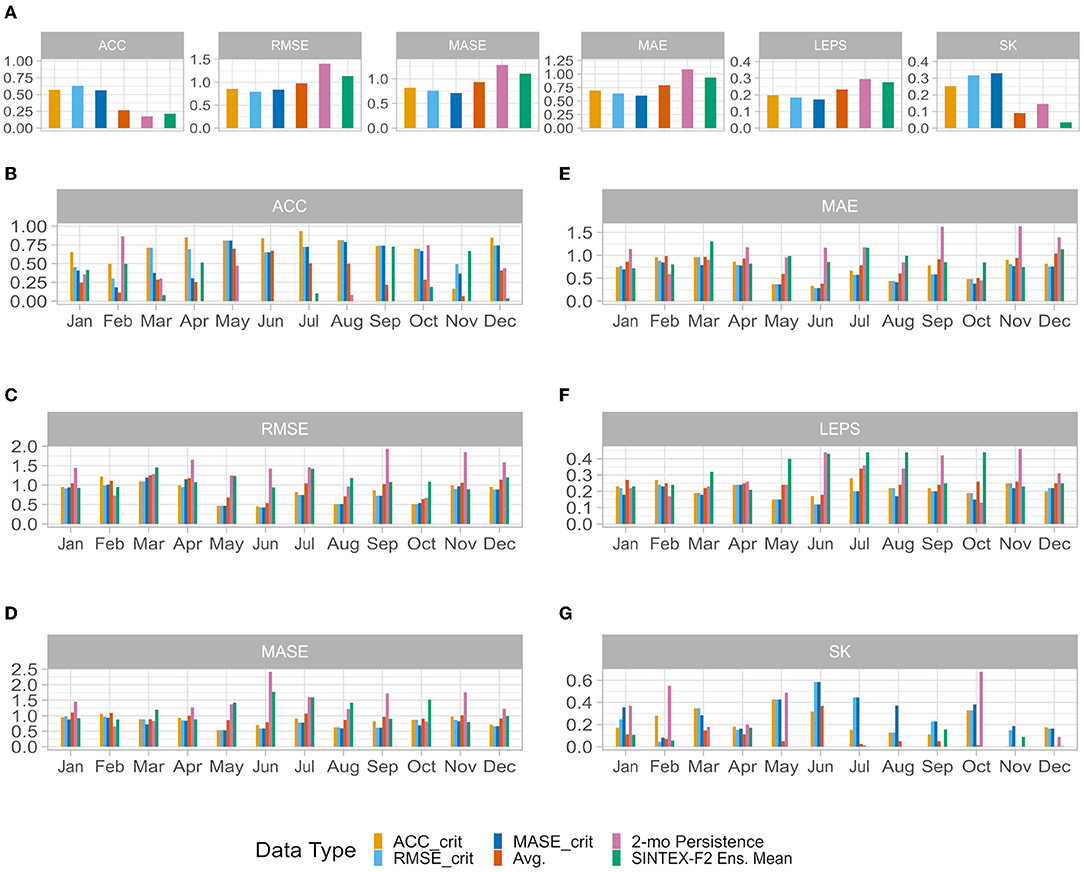
Figure 9. Evaluation of the different prediction systems performance including the 2-month persistence (pink) and SINTEX-F2 (lime green). (A) Overall performance over the complete validation period, showing the anomaly correlation coefficient (ACC), root mean square error (RMSE), mean absolute scaled error (MASE), mean absolute error (MAE), linear error in probability space (LEPS), and skill error (SK). (B–F) Individual monthly performance metrics. Monthly performance according to (B) ACC, (C) RMSE, (D) MASE, (E) MAE, (F) LEPS, and (G) SK.
Interestingly, while all three optimized models perform equally well over the validation period (with the model based on ACC_crit slightly left behind), the average of the 72 models performs less well though still better than the SINTEX-F2 ensemble mean and the 2-month lead persistence (Figure 9A). The selective ensemble mean technique (Ratnam et al., 2021a) may help to improve the average of the 72 models by carefully only picking the models with enough skills, before calculating the average.
The monthly stratification reveals the abilities and limitations of the hybrid prediction systems, and their disparities. In late spring, summer, and fall, simulated SAT are close to the observed ones (i.e., along the 1:1 line in Figure 8B), indicating that the hybrid systems perform quite well. ACCs are close to 0.75 during these seasons for most of the optimized models (Figure 9B). This is confirmed by other metrics, RMSE (Figure 9C), MASE (Figure 9D), MAE (Figure 9E), and LEPS (Figure 9F) are very low compared to other months. Also, the SKs are maximum during the same months (Figure 9G). This clearly indicates that the hybrid systems perform better than the SINTEX-F2 ensemble mean as well as the persistence predictions during these months. In late fall, winter (with the exception of December) and early spring, on the other hand, performance as measured by the ACC and other metrics is not as high as in other seasons. Thus, it seems the hybrid models are less able to predict the sign of the interannual anomalies, as well as their intensity during the cold period. Nevertheless, even for the non-ACC metrics, the hybrid model still outperforms the SINTEX-F2 ensemble mean and the persistence. Along the year, the ensemble average of the hybrid models struggles to reproduce the intensity of the anomalies (“Avg.” line, Figure 8C), with a weak forecast amplitude most of the time. Individual hybrid systems have better results (but suffer from other problems, such as overestimating anomalies in February). It is also confirmed that SAT in February and November are not very well-simulated, with the lowest ACC (Figure 9B) among all months, and poor performance in other metrics as well (Figures 9C–G).
Summary and Discussion
We have presented a novel approach that combines dynamical forecasts with machine learning to predict SAT anomalies over the Kantō region, a part of the central region of Japan. In this approach, the role of the machine learning is to represent the influences of remote SST, which are not well-simulated in the dynamical model.
Results of this HPS are promising, particularly because they outperform both the 2-month lead persistence and the SINTEX-F2 forecasts of the SAT in the Kantō region, indicating the (linear and non-linear) teleconnections have been (partially) restored in this method. Results also suggest that the hybrid approach is able to improve prediction skill in mid-latitudes. The HPS was able to quite accurately forecast the SAT of the evaluation subset, particularly the rapid change of sign between March 2020 and July 2020 (Figure 8B). This is very encouraging, as the HPS seems to address the overfitting issue and to create a good compromise between interpretability and accuracy (Section Limitations). It also performed quite well in winter, but missed the correct sign of October 2020 and the intensity of August 2020 and March 2021 (while correct in sign).
Another interesting result is the share (about 50%) of boosting methods in the HPS, outperforming seminal methods such as artificial neural networks. It is also worth noting that the support vector machine algorithms are also picked up during the optimization phase. The remaining selected methods are distributed random forest and CatBoost. The Bayesian approach is never picked up as the best solution (at least in our study design).
Some previous studies have already discussed the prediction of SAT in Japan, either by selecting the best from the SINTEX-F2 predictions the best ensemble members with regard to the SAT (Ratnam et al., 2021a), or by using past observations of SST to predict winter SAT with the help of ANN (Ratnam et al., 2021b). While a direct comparison of the results is difficult due to the differing approach and study regions, the forecast skills in winter are quite comparable. We recognize a potential application could be to combine these prediction systems, for example by selecting the best systems (based on accuracy measurement) or by weighting the forecasts (Bates and Granger, 1969; Aiolfi and Timmermann, 2006; Aiolfi et al., 2010; Hsiao and Wan, 2014). This will be explored in a future study.
On the other hand, the results also show some limitations of this approach. Even though the HPS outperforms the dynamical forecast system, it can only reproduce around 35–40% of the variance of the Kantō SAT index between 2010 and 2020.
This suggests that model improvement may be obtained by including additional variables, such as the geopotential height, to take into account the atmospheric dynamics, which are likely to play a role in the SAT variability, as well as soil moisture, which is a key variable in the occurrence of temperature extremes (Seneviratne et al., 2010; Quesada et al., 2012). In some years, as seen in Figure 8A, the HPS could not correctly predict the SAT index in the Kantō region. Exploring the reasons of these forecast failures could help to improve the HPS by adding supplementary information, such as atmospheric processes. Adding more variables and introducing time lags will likely increase the amount of information to analyze, and using deep learning algorithms may help to improve the seasonal forecast by revealing unknown interactions among variables. We would also like to add that deep-learning could in fact be used as a tool for prediction (with feature selection to avoid redundancy in the information). But it could also be used as an analysis tool to document the relationships between variables, particularly through the use of layer-wise relevance propagation (LRP) or heat maps (Bach et al., 2015; Zhou et al., 2016; Montavon et al., 2019; Toms et al., 2020). LRPs quantifies the contributions of the predictors to the predictand, providing a physical interpretation.
The HPS approach is based on the strong assumptions that (1) the explanatory power of the predictors selected in each monthly model is robust in time i.e., we assume that the selection during the calibration of the models is valid for the validation period and, most importantly, for the future. (2) Although the model seems to be robust over different time periods, it relies on the accurate seasonal prediction of SST, particularly outside the tropical region where SINTEX-F2 has more limited skills.
ML algorithms used in this study have a relatively low risk of over-fitting, but because of the limited sample size for calibration, over-fitting cannot be totally avoided, which may explain the limited skills of the hybrid model in some months.
A possible drawback of the HPS is the limitation in deriving physical interpretation from the monthly models as by construction, potential sources of predictability from the global ocean are included, regardless of physical distance to the target region. Due this limitation, it is still difficult to derive physical mechanisms from ML (Section Limitations). Such physical understanding will eventually help to improve prediction skill and should be therefore addressed in future studies.
Data Availability Statement
The datasets presented in this article are not readily available because of confidentiality agreements. Supporting SINTEX-F2 model data can only be made available to bona fide researcher's subject to a non-disclosure agreement. Details of the data and how to request access are available from the authors. Monthly mean surface air temperatures are available by contacting the Japanese Meteorological Agency (JMA). The list of the stations used in this work is available from the authors. Requests to access the datasets should be directed to SINTEX-F2: Takeshi Doi, takeshi.doi@jamstec.go.jp; Monthly mean surface air temperatures: https://www.jma.go.jp/jma/indexe.html.
Author Contributions
HK, YT, and IH initiated the internal project. PO, MN, IR, and SB contributed to conception and design of the study. PO performed the statistical analysis and wrote the first draft of the manuscript. All authors contributed to manuscript revision, read, and approved the submitted version.
Funding
This research was partly supported by JERA Co., Inc.
Conflict of Interest
HK, YT, and IH were employed by the company JERA Co., Inc. This study received funding from JERA Co., Inc. The funder had the following involvement with the study: decision to publish and preparation of the manuscript.
The remaining authors declare that the research was conducted in the absence of any commercial or financial relationships that could be construed as a potential conflict of interest.
Publisher's Note
All claims expressed in this article are solely those of the authors and do not necessarily represent those of their affiliated organizations, or those of the publisher, the editors and the reviewers. Any product that may be evaluated in this article, or claim that may be made by its manufacturer, is not guaranteed or endorsed by the publisher.
Acknowledgments
The authors would like to thank Dr. Takeshi Doi (APL VAiG, JAMSTEC, Japan) for providing the SINTEX-F2 data. The authors are also grateful to Japanese Meteorological Agency for providing dataset.
References
Aiolfi, M., Capistrán, C., and Timmermann, A. (2010). Forecast Combinations. Rochester, NY: Social Science Research Network. doi: 10.2139/ssrn.1609530
Aiolfi, M., and Timmermann, A. (2006). Persistence in forecasting performance and conditional combination strategies. J. Econom. 135, 31–53. doi: 10.1016/j.jeconom.2005.07.015
Akihiko, T., Morioka, Y., and Behera, S. K. (2014). Role of climate variability in the heatstroke death rates of Kantō region in Japan. Sci. Rep. 4:5655. doi: 10.1038/srep05655
Auffhammer, M. (2014). Cooling China: the weather dependence of air conditioner adoption. Front. Econ. China 9, 70–84. doi: 10.3868/s060-003-014-0005-5
Auffhammer, M., and Aroonruengsawat, A. (2012). Hotspots of Climate-Driven Increases in Residential Electricity Demand: A Simulation Exercise Based on Household Level Billing Data for California. California Energy Commission. Available online at: https://escholarship.org/uc/item/98x2n4rs (accessed September 16, 2021).
Auffhammer, M., and Mansur, E. T. (2014). Measuring climatic impacts on energy consumption: a review of the empirical literature. Energy Econ. 46, 522–530. doi: 10.1016/j.eneco.2014.04.017
Bach, S., Binder, A., Montavon, G., Klauschen, F., Müller, K.-R., and Samek, W. (2015). On pixel-wise explanations for non-linear classifier decisions by layer-wise relevance propagation. PLoS ONE 10:e0130140. doi: 10.1371/journal.pone.0130140
Bai, C., Zhang, R., Bao, S., Liang, X. S., and Guo, W. (2018). Forecasting the tropical cyclone genesis over the Northwest Pacific through identifying the causal factors in cyclone–climate interactions. J. Atmos. Oceanic Technol. 35, 247–259. doi: 10.1175/JTECH-D-17-0109.1
Barnard, G. A. (1986). “Causation,” in Encyclopedia of Statistical Sciences, eds S. Kotz and N. L. Johnson (New York, NY: John Wiley and Sons),387–389.
Barnston, A. G. (1994). Linear statistical short-term climate predictive skill in the Northern Hemisphere. J. Clim. 7, 1513–1564. doi: 10.1175/1520-0442(1994)007<1513:LSSTCP>2.0.CO
Bates, J. M., and Granger, C. W. J. (1969). The combination of forecasts. Oper. Res. Q. 20, 451–468. doi: 10.2307/3008764
Bergmeir, C., and Benítez, J. M. (2012). Neural networks in R using the stuttgart neural network simulator: RSNNS. J. Stat. Softw. 46, 1–26. doi: 10.18637/jss.v046.i07
Bergstra, J., and Bengio, Y. (2012). Random search for hyper-parameter optimization. J. Mach. Learn. Res. 13, 281–305.
Branković, C., Palmer, T. N., Molteni, F., Tibaldi, S., and Cubasch, U. (1990). Extended-range predictions with ECMWF models: time-lagged ensemble forecasting. Q. J. R. Meteorol. Soc. 116, 867–912. doi: 10.1002/qj.49711649405
Breiman, L., Friedman, J. H., Olshen, R. A., and Stone, C. J. (1984). Classification and Regression Trees. New York, NY: Routledge. doi: 10.1201/9781315139470
Carriquiry, M. A., and Osgood, D. E. (2012). Index insurance, probabilistic climate forecasts, and production. J. Risk Insur. 79, 287–300. doi: 10.1111/j.1539-6975.2011.01422.x
Ceglar, A., and Toreti, A. (2021). Seasonal climate forecast can inform the European agricultural sector well in advance of harvesting. npj Clim. Atmos. Sci. 4, 42–49. doi: 10.1038/s41612-021-00198-3
Changnon, D., Creech, T., Marsili, N., Murrell, W., and Saxinger, M. (1999). Interactions with a weather-sensitive decision maker: a case study incorporating ENSO information into a strategy for purchasing natural gas. Bull. Amer. Meteor. Soc. 80, 1117–1126. doi: 10.1175/1520-0477(1999)080<1117:IWAWSD>2.0.CO
Chantry, M., Christensen, H., Dueben, P., and Palmer, T. (2021). Opportunities and challenges for machine learning in weather and climate modelling: hard, medium and soft AI. Philos. Trans. R. Soc. A Math. Phys. Eng. Sci. 379:20200083. doi: 10.1098/rsta.2020.0083
Chattopadhyay, S., Jhajharia, D., and Chattopadhyay, G. (2011). Univariate modelling of monthly maximum temperature time series over northeast India: neural network versus Yule–Walker equation based approach. Meteorol. Appl. 18, 70–82. doi: 10.1002/met.211
Chelton, D. B. (1983). Effects of sampling errors in statistical estimation. Deep Sea Res. Part I Oceanogr. Res. Pap. 30, 1083–1103. doi: 10.1016/0198-0149(83)90062-6
Chen, T., and Guestrin, C. (2016). “XGBoost: A scalable tree boosting system,” in Proceedings of the 22nd ACM SIGKDD International Conference on Knowledge Discovery and Data Mining (San Francisco, CA), 785–794. doi: 10.1145/2939672.2939785
Chen, T., He, T., Benesty, M., Khotilovich, V., Tang, Y., Cho, H., et al. (2020). xgboost: Extreme Gradient Boosting. Available online at: https://github.com/dmlc/xgboost (accessed February 19, 2020).
Chipman, H. A., George, E. I., and McCulloch, R. E. (2010). BART: Bayesian additive regression trees. Ann. Appl. Stat. 4, 266–298. doi: 10.1214/09-AOAS285
Cifuentes, J., Marulanda, G., Bello, A., and Reneses, J. (2020). Air temperature forecasting using machine learning techniques: a review. Energies 13:4215. doi: 10.3390/en13164215
Darbyshire, R., Crean, J., Cashen, M., Anwar, M. R., Broadfoot, K. M., Simpson, M., et al. (2020). Insights into the value of seasonal climate forecasts to agriculture. Aust. J. Agric. Resour. Econ. 64, 1034–1058. doi: 10.1111/1467-8489.12389
Davis, R. E. (1976). Predictability of sea surface temperature and sea level pressure anomalies over the north Pacific Ocean. J. Phys. Oceanogr. 6, 249–266. doi: 10.1175/1520-0485(1976)006<0249:POSSTA>2.0.CO;2
Diebold, F. X., and Mariano, R. S. (1995). Comparing predictive accuracy. J. Bus. Econ. Statist. 13, 253–263. doi: 10.1080/07350015.1995.10524599
Dijkstra, H. A., Petersik, P., Hernández-García, E., and López, C. (2019). The application of machine learning techniques to improve El Niño prediction skill. Front. Phys. 7:153. doi: 10.3389/fphy.2019.00153
Doblas-Reyes, F. J., García-Serrano, J., Lienert, F., Biescas, A. P., and Rodrigues, L. R. L. (2013). Seasonal climate predictability and forecasting: status and prospects. WIREs Clim. Change 4, 245–268. doi: 10.1002/wcc.217
Doi, T., Behera, S. K., and Yamagata, T. (2016). Improved seasonal prediction using the SINTEX-F2 coupled model. J. Adv. Model. Earth Syst. 8, 1847–1867. doi: 10.1002/2016MS000744
Doi, T., Storto, A., Behera, S. K., Navarra, A., and Yamagata, T. (2017). Improved prediction of the indian ocean dipole mode by use of subsurface ocean observations. J. Clim. 30, 7953–7970. doi: 10.1175/JCLI-D-16-0915.1
Dorogush, A. V., Ershov, V., and Gulin, A. (2018). CatBoost: gradient boosting with categorical features support. arXiv 1–7.
Drosdowsky, W., and Chambers, L. E. (2001). Near-global sea surface temperature anomalies as predictors of Australian seasonal rainfall. J. Clim. 14, 1677–1687. doi: 10.1175/1520-0442(2001)014<1677:NACNGS>2.0.CO;2
Eade, R., Smith, D., Scaife, A., Wallace, E., Dunstone, N., Hermanson, L., et al. (2014). Do seasonal-to-decadal climate predictions underestimate the predictability of the real world? Geophys. Res. Lett. 41, 5620–5628. doi: 10.1002/2014GL061146
Efron, B. (1979). Bootstrap methods: another look at the jackknife. Ann. Statist. 7, 1–26. doi: 10.1214/aos/1176344552
Efron, B. (1983). Estimating the error rate of a prediction rule: improvement on cross-validation. J. Amer. Statist. Assoc. 78, 316–331. doi: 10.2307/2288636
Efron, B., and Tibshirani, R. (1997). Improvements on cross-validation: The .632+ Bootstrap method. J. Amer. Statist. Assoc. 92, 548–560. doi: 10.2307/2965703
Fan, Y., and van den Dool, H. (2008). A global monthly land surface air temperature analysis for 1948-present. J. Geophys. Res. 113, 1–18. doi: 10.1029/2007JD008470
Fox, J., and Monette, G. (1992). Generalized collinearity diagnostics. J. Amer. Statist. Assoc. 87, 178–183. doi: 10.2307/2290467
Franses, P. H. (2016). A note on the mean absolute scaled error. Int. J. Forecast. 32, 20–22. doi: 10.1016/j.ijforecast.2015.03.008
Friedman, J. H. (1999a). Greedy Function Approximation: A Gradient Boosting Machine. Standford, CA: Standford University. Available online at: https://statweb.stanford.edu/j~hf/ftp/trebst.pdf (accessed November 30, 2020).
Friedman, J. H. (1999b). Stochastic Gradient Boosting. Standford, CA: Standford University Available online at: https://statweb.stanford.edu/j~hf/ftp/stobst.pdf (accessed November 30, 2020).
Fritsch, J. M., Hilliker, J., Ross, J., and Vislocky, R. L. (2000). Model consensus. Wea. Forecast. 15, 571–582. doi: 10.1175/1520-0434(2000)015<0571:MC>2.0.CO;2
Fritsch, S., Guenther, F., and Wright, M. N. (2019). Neuralnet: Training of Neural Networks. Available online at: https://CRAN.R-project.org/package=neuralnet (accessed October 29, 2021).
Gibson, P. B., Chapman, W. E., Altinok, A., Delle Monache, L., DeFlorio, M. J., and Waliser, D. E. (2021). Training machine learning models on climate model output yields skillful interpretable seasonal precipitation forecasts. Commun. Earth Environ. 2:159. doi: 10.1038/s43247-021-00225-4
Goddard, L., Mason, S. J., Zebiak, S. E., Ropelewski, C. F., Basher, R., and Cane, M. A. (2001). Current approaches to seasonal to interannual climate predictions. Int. J. Climatol. 21, 1111–1152. doi: 10.1002/joc.636
Granger, C. W. J. (1969). Investigating causal relations by econometric models and cross-spectral methods. Econometrica 37, 424–438. doi: 10.2307/1912791
Gunasekera, D. (2018). “Bridging the energy and meteorology information gap,” in Weather and Climate Services for the Energy Industry, ed A. Troccoli (Cham: Springer International Publishing), 1–12. doi: 10.1007/978-3-319-68418-5_1
Hagedorn, R., Doblas-Reyes, F. J., and Palmer, T. N. (2005). The rationale behind the success of multi-model ensembles in seasonal forecasting—I. Basic concept. Tellus A 57, 219–233. doi: 10.1111/j.1600-0870.2005.00103.x
Ham, Y.-G., Kim, J.-H., and Luo, J.-J. (2019). Deep learning for multi-year ENSO forecasts. Nature 573, 568–572. doi: 10.1038/s41586-019-1559-7
Hancock, J. T., and Khoshgoftaar, T. M. (2020). CatBoost for big data: an interdisciplinary review. J. Big Data 7:94. doi: 10.1186/s40537-020-00369-8
Hansen, J. W. (2002). Realizing the potential benefits of climate prediction to agriculture: issues, approaches, challenges. Agric. Syst. 74, 309–330. doi: 10.1016/S0308-521X(02)00043-4
Hastie, T., Tibshirani, R., and Friedman, J. H. (2009). The Elements of Statistical Learning: Data Mining, Inference, and Prediction, 2nd Edn. New York, NY: Springer.
Henderson, S. A., Maloney, E. D., and Son, S.-W. (2017). Madden–Julian oscillation pacific teleconnections: the impact of the basic state and MJO representation in general circulation models. J. Clim. 30, 4567–4587. doi: 10.1175/JCLI-D-16-0789.1
Hsiao, C., and Wan, S. K. (2014). Is there an optimal forecast combination? J. Econom. 178, 294–309. doi: 10.1016/j.jeconom.2013.11.003
Hyndman, R. J. (2006). Another look at forecast-accuracy metrics for intermittent demand. Foresight. 4, 43–46. Available online at: https://robjhyndman.com/papers/foresight.pdf
Hyndman, R. J., and Koehler, A. B. (2006). Another look at measures of forecast accuracy. Int. J. Forecast. 22, 679–688. doi: 10.1016/j.ijforecast.2006.03.001
Ibrahim, A. A., Ridwan, R. L., Muhammed, M. M., Abdulaziz, R. O., and Saheed, G. A. (2020). Comparison of the catboost classifier with other machine learning methods. IJACSA. 11, 738–748. doi: 10.14569/IJACSA.2020.0111190
Jabeur, S. B., Gharib, C., Mefteh-Wali, S., and Arfi, W. B. (2021). CatBoost model and artificial intelligence techniques for corporate failure prediction. Technol. Forecast. Soc. Change 166:120658. doi: 10.1016/j.techfore.2021.120658
James, G., Witten, D., Hastie, T., and Tibshirani, R. (2013). An Introduction to Statistical Learning. New York, NY: Springer. doi: 10.1007/978-1-4614-7138-7
Japanese Meteorological Agency (2018). Comments on Meteorological Observation Statistics [in Japanese]. Tokyo: Japan Meteorological Agency. Available online at: https://www.data.jma.go.jp/obd/stats/data/kaisetu/shishin/shishin_all.pdf (accessed March 28, 2019).
Jin, E. K., Kinter, J. L., Wang, B., Park, C.-K., Kang, I.-S., Kirtman, B. P., et al. (2008). Current status of ENSO prediction skill in coupled ocean–atmosphere models. Clim. Dyn. 31, 647–664. doi: 10.1007/s00382-008-0397-3
Kapelner, A., and Bleich, J. (2016). BARTmachine: machine learning with bayesian additive regression trees. J. Stat. Softw. 70, 1–40. doi: 10.18637/jss.v070.i04
Karatzoglou, A., Smola, A., Hornik, K., and Zeileis, A. (2004). kernlab – An S4 package for kernel methods in R. J. Stat. Softw. 11, 1–20. doi: 10.18637/jss.v011.i09
Kuhn, M. (2020). Caret: Classification and regression training. Available online at: https://CRAN.R-project.org/package=caret (accessed January 12, 2021).
Kuhn, M., and Johnson, K. (2016). Applied Predictive Modeling. Corrected at 5th Printing. New York, NY: Springer. doi: 10.1007/978-1-4614-6849-3
Kumar, A. (2010). On the assessment of the value of the seasonal forecast information. Meteorol. Appl. 17, 385–392. doi: 10.1002/met.167
Kursa, M. B., Aleksander, J., and Rudnicki, W. R. (2010). Boruta – a system for feature selection. Fundam. Inform. 101, 271–285. doi: 10.3233/FI-2010-288
Kursa, M. B., and Rudnicki, W. R. (2010). Feature selection with the Boruta package. J. Stat. Softw. 36, 1–13. doi: 10.18637/jss.v036.i11
Lakshmanan, V., Gilleland, E., McGovern, A., and Tingley, M., (Eds.). (2015). Machine Learning and Data Mining Approaches to Climate Science: Proceedings of the 4th International Workshop on Climate Informatics. Cham; Heidelberg; New York, NY: Springer.
Leblois, A., and Quirion, P. (2013). Agricultural insurances based on meteorological indices: realizations, methods and research challenges. Meteorol. Appl. 20, 1–9. doi: 10.1002/met.303
Liang, X. S. (2008). Information flow within stochastic dynamical systems. Phys. Rev. E 78:031113. doi: 10.1103/PhysRevE.78.031113
Liang, X. S. (2014). Unraveling the cause-effect relation between time series. Phys. Rev. E 90, 052150. doi: 10.1103/PhysRevE.90.052150
Liang, X. S. (2015). Normalizing the causality between time series. Phys. Rev. E 92:022126. doi: 10.1103/PhysRevE.92.022126
Liang, X. S. (2016). Information flow and causality as rigorous notions ab initio. Phys. Rev. E 94:052201. doi: 10.1103/PhysRevE.94.052201
Liang, X. S. (2019). A study of the cross-scale causation and information flow in a stormy model mid-latitude atmosphere. Entropy 21:149. doi: 10.3390/e21020149
Liang, X. S., and Kleeman, R. (2007a). A rigorous formalism of information transfer between dynamical system components. I. Discrete mapping. Phys. D 231, 1–9. doi: 10.1016/j.physd.2007.04.002
Liang, X. S., and Kleeman, R. (2007b). A rigorous formalism of information transfer between dynamical system components. II. Continuous flow. Phys. D 227, 173–182. doi: 10.1016/j.physd.2006.12.012
Livezey, R. E. (1990). Variability of skill of long-range forecasts and implications for their use and value. Bull. Amer. Meteor. Soc. 71, 300–309. doi: 10.1175/1520-0477(1990)071<0300:VOSOLR>2.0.CO;2
Luo, J.-J., Masson, S., Behera, S., and Yamagata, T. (2007). Experimental forecasts of the Indian ocean dipole using a coupled OAGCM. J. Clim. 20, 2178–2190. doi: 10.1175/JCLI4132.1
Luo, J.-J., Masson, S., Behera, S. K., Shingu, S., and Yamagata, T. (2005). Seasonal climate predictability in a coupled OAGCM using a different approach for ensemble forecasts. J. Clim. 18, 4474–4497. doi: 10.1175/JCLI3526.1
Luo, J.-J., Masson, S., Behera, S. K., and Yamagata, T. (2008b). Extended ENSO predictions using a fully coupled ocean–atmosphere model. J. Clim. 21, 84–93. doi: 10.1175/2007JCLI1412.1
Luo, J. -J., Behera, S., Masumoto, Y., Sakuma, H., and Yamagata, T. (2008a). Successful prediction of the consecutive IOD in 2006 and 2007. Geophys. Res. Lett. 35, 1–6. doi: 10.1029/2007GL032793
Luo, M., Wang, Y., Xie, Y., Zhou, L., Qiao, J., Qiu, S., et al. (2021). Combination of feature selection and CatBoost for prediction: the first application to the estimation of aboveground biomass. Forests 12:216. doi: 10.3390/f12020216
Makridakis, S., Spiliotis, E., and Assimakopoulos, V. (2018). Statistical and machine learning forecasting methods: concerns and ways forward. PLoS ONE 13:e0194889. doi: 10.1371/journal.pone.0194889
Marquardt, D. W. (1970). Generalized inverses, ridge regression, biased linear estimation, and nonlinear estimation. Technometrics 12, 591–612. doi: 10.1080/00401706.1970.10488699
McGovern, A., Lagerquist, R., John Gagne, D., Jergensen, G. E., Elmore, K. L., Homeyer, C. R., et al. (2019). Making the black box more transparent: understanding the physical implications of machine learning. Bull. Amer. Meteor. Soc. 100, 2175–2199. doi: 10.1175/BAMS-D-18-0195.1
Meza, F. J., Hansen, J. W., and Osgood, D. (2008). Economic value of seasonal climate forecasts for agriculture: review of ex-ante assessments and recommendations for future research. J. Appl. Meteor. Climatol. 47, 1269–1286. doi: 10.1175/2007JAMC1540.1
Milton, S. F. (1990). Practical extended-range forecasting using dynamical models. Meteorol. Mag 119, 221–233.
Ministry of Internal Affairs Communications (2020). Statistical Observations of Municipalities [in Japanese]. Tokyo: Statistics Bureau, Ministry of Internal Affairs and communications. Available online at: https://www.stat.go.jp/data/s-sugata/ (accessed December 7, 2020).
Montavon, G., Binder, A., Lapuschkin, S., Samek, W., and Müller, K.-R. (2019). “Layer-wise relevance propagation: an overview,” in Explainable AI: Interpreting, Explaining and Visualizing Deep Learning Lecture Notes in Computer Science, eds W. Samek, G. Montavon, A. Vedaldi, L. K. Hansen, and K.-R. Müller (Cham: Springer International Publishing), 193–209. doi: 10.1007/978-3-030-28954-6_10
Monteleoni, C., Schmidt, G. A., and McQuade, S. (2013). Climate informatics: accelerating discovering in climate science with machine learning. Comput. Sci. Eng. 15, 32–40. doi: 10.1109/MCSE.2013.50
Mori, H., and Kanaoka, D. (2007). “Application of support vector regression to temperature forecasting for short-term load forecasting,” in 2007 International Joint Conference on Neural Networks (Orlando, FL), 1085–1090. doi: 10.1109/IJCNN.2007.4371109
Oettli, P., Nonaka, M., Kuroki, M., Koshiba, H., Tokiya, Y., and Behera, S. K. (2021). Understanding global teleconnections to surface air temperatures in Japan based on a new climate classification. Int. J. Climatol. 41, 1112–1127. doi: 10.1002/joc.6754
Oludhe, C., Sankarasubramanian, A., Sinha, T., Devineni, N., and Lall, U. (2013). The role of multimodel climate forecasts in improving water and energy management over the Tana River Basin, Kenya. J. Appl. Meteor. Climatol. 52, 2460–2475. doi: 10.1175/JAMC-D-12-0300.1
Osgood, D. E., Suarez, P., Hansen, J., Carriquiry, M., and Mishra, A. (2008). Integrating Seasonal Forecasts and Insurance for Adaptation among Subsistence Farmers: The Case of Malawi. Washington, DC: World Bank. Available online at: https://openknowledge.worldbank.org/handle/10986/6873 (accessed December 8, 2020).
Pepler, A. S., Díaz, L. B., Prodhomme, C., Doblas-Reyes, F. J., and Kumar, A. (2015). The ability of a multi-model seasonal forecasting ensemble to forecast the frequency of warm, cold and wet extremes. Weather Clim. Extremes 9, 68–77. doi: 10.1016/j.wace.2015.06.005
Potts, J. M., Folland, C. K., Jolliffe, I. T., and Sexton, D. (1996). Revised “LEPS” scores for assessing climate model simulations and long-range forecasts. J. Clim. 9, 34–53. doi: 10.1175/1520-0442(1996)009<0034:RSFACM>2.0.CO;2
Prokhorenkova, L., Gusev, G., Vorobev, A., Dorogush, A. V., and Gulin, A. (2019). CatBoost: unbiased boosting with categorical features. arXiv 1–23.
Quesada, B., Vautard, R., Yiou, P., Hirschi, M., and Seneviratne, S. I. (2012). Asymmetric European summer heat predictability from wet and dry southern winters and springs. Nat. Clim. Change 2, 736–741. doi: 10.1038/nclimate1536
R Core Team (2019). R: A Language and Environment for Statistical Computing. Vienna: R Foundation for Statistical Computing. Available online at: https://www.R-project.org/ (accessed April 1, 2021).
Ratnam, J. V., Doi, T., Morioka, Y., Oettli, P., Nonaka, M., and Behera, S. K. (2021a). Improving predictions of surface air temperature anomalies over japan by the selective ensemble mean technique. Weather Forecast. 36, 207–217. doi: 10.1175/WAF-D-20-0109.1
Ratnam, J. V., Nonaka, M., and Behera, S. K. (2021b). Winter surface air temperature prediction over Japan using artificial neural networks. Weather Forecast. 36, 1343–1356. doi: 10.1175/WAF-D-20-0218.1
Raudys, S. J., and Jain, A. K. (1991). Small sample size effects in statistical pattern recognition: recommendations for practitioners. IEEE Trans. Pattern Anal. Mach. Intell. 13, 252–264. doi: 10.1109/34.75512
Salcedo-Sanz, S., Deo, R. C., Carro-Calvo, L., and Saavedra-Moreno, B. (2016). Monthly prediction of air temperature in Australia and New Zealand with machine learning algorithms. Theor. Appl. Climatol. 125, 13–25. doi: 10.1007/s00704-015-1480-4
Schepen, A., Wang, Q. J., and Robertson, D. E. (2012). Combining the strengths of statistical and dynamical modeling approaches for forecasting Australian seasonal rainfall. J. Geophys. Res. Atmos. 117:D20107. doi: 10.1029/2012JD018011
Schreiber, T. (2000). Measuring information transfer. Phys. Rev. Lett. 85, 461–464. doi: 10.1103/PhysRevLett.85.461
Seneviratne, S. I., Corti, T., Davin, E. L., Hirschi, M., Jaeger, E. B., Lehner, I., et al. (2010). Investigating soil moisture–climate interactions in a changing climate: a review. Earth Sci. Rev. 99, 125–161. doi: 10.1016/j.earscirev.2010.02.004
Shannon, C. E. (1948). A mathematical theory of communication. Bell Syst. Tech. J. 27, 623–666. doi: 10.1002/j.1538-7305.1948.tb00917.x
Sheffield, J., Barrett, A. P., Colle, B., Fernando, D. N., Fu, R., Geil, K. L., et al. (2013a). North American climate in CMIP5 experiments. Part I: evaluation of historical simulations of continental and regional climatology*. J. Clim. 26, 9209–9245. doi: 10.1175/JCLI-D-12-00592.1
Sheffield, J., Camargo, S. J., Fu, R., Hu, Q., Jiang, X., Johnson, N., et al. (2013b). North American climate in CMIP5 experiments. Part II: evaluation of historical simulations of intraseasonal to decadal variability. J. Clim. 26, 9247–9290. doi: 10.1175/JCLI-D-12-00593.1
Shukla, J. (1985). “Predictability,” in Advances in Geophysics (Elsevier), 87–122. doi: 10.1016/S0065-2687(08)60186-7
Shukla, J. (1998). Predictability in the midst of chaos: a scientific basis for climate forecasting. Science 282, 728–731. doi: 10.1126/science.282.5389.728
Shukla, J., and Kinter, J. L. (2006). “Predictability of seasonal climate variations: a pedagogical review,” in Predictability of Weather and Climate, eds R. Hagedorn and T. Palmer (Cambridge: Cambridge University Press), 306–341. doi: 10.1017/CBO9780511617652.013
Smith, B. A., Hoogenboom, G., and McClendon, R. W. (2009). Artificial neural networks for automated year-round temperature prediction. Comput. Electron. Agric. 68, 52–61. doi: 10.1016/j.compag.2009.04.003
Soares, M. B., Daly, M., and Dessai, S. (2018). Assessing the value of seasonal climate forecasts for decision-making. WIREs Clim. Change 9:e523. doi: 10.1002/wcc.523
Stips, A., Macias, D., Coughlan, C., Garcia-Gorriz, E., and Liang, X. S. (2016). On the causal structure between CO2 and global temperature. Sci. Rep. 6:21691. doi: 10.1038/srep21691
Stockdale, T. N., Anderson, D. L. T., Balmaseda, M. A., Doblas-Reyes, F., Ferranti, L., Mogensen, K., et al. (2011). ECMWF seasonal forecast system 3 and its prediction of sea surface temperature. Clim. Dyn. 37, 455–471. doi: 10.1007/s00382-010-0947-3
Sugihara, G., May, R., Ye, H., Hsieh, C., Deyle, E. R., Fogarty, M., et al. (2012). Detecting causality in complex ecosystems. Science 338, 496–500. doi: 10.1126/science.1227079
Toms, B. A., Barnes, E. A., and Ebert-Uphoff, I. (2020). Physically interpretable neural networks for the geosciences: applications to earth system variability. J. Adv. Model. Earth Syst. 12:e2019MS002002. doi: 10.1029/2019MS002002
Tran, T. T. K., Bateni, S. M., Ki, S. J., and Vosoughifar, H. (2021). A review of neural networks for air temperature forecasting. Water 13:1294. doi: 10.3390/w13091294
Troccoli, A., Harrison, M., Anderson, D. L. T., and Mason, S. J., (Eds.). (2008). Seasonal Climate: Forecasting and Managing Risk. Dordrecht: Springer.
Tsonis, A. A., and Roebber, P. J. (2004). The architecture of the climate network. Phys. A Statist. Mech. Appl. 333, 497–504. doi: 10.1016/j.physa.2003.10.045
Ustaoglu, B., Cigizoglu, H. K., and Karaca, M. (2008). Forecast of daily mean, maximum and minimum temperature time series by three artificial neural network methods. Meteorol. Appl. 15, 431–445. doi: 10.1002/met.83
van der Ploeg, T., Austin, P. C., and Steyerberg, E. W. (2014). Modern modelling techniques are data hungry: a simulation study for predicting dichotomous endpoints. BMC Med. Res. Methodol. 14:137. doi: 10.1186/1471-2288-14-137
Venables, W. N., and Ripley, B. D. (2002). Modern Applied Statistics with S. New York, NY: Springer.
Voyant, C., Notton, G., Kalogirou, S., Nivet, M.-L., Paoli, C., Motte, F., et al. (2017). Machine learning methods for solar radiation forecasting: a review. Renew. Energ. 105, 569–582. doi: 10.1016/j.renene.2016.12.095
Ward, M. N., and Folland, C. K. (1991). Prediction of seasonal rainfall in the north Nordeste of Brazil using eigenvectors of sea-surface temperature. Int. J. Climatol. 11, 711–743. doi: 10.1002/joc.3370110703
Willmott, C. J., and Matsuura, K. (2005). Advantages of the mean absolute error (MAE) over the root mean square error (RMSE) in assessing average model performance. Clim. Res. 30, 79–82. doi: 10.3354/cr030079
World Health Organization (2015). Indoor Residual Spraying: An Operational Manual for Indoor Residual Spraying (IRS) for Malaria Transmission Control and Elimination, 2nd Edn. Geneva: World Health Organization. Available online at: https://apps.who.int/iris/handle/10665/177242 (accessed December 7, 2021).
Xia, Y., He, L., Li, Y., Liu, N., and Ding, Y. (2020). Predicting loan default in peer-to-peer lending using narrative data. J. Forecast. 39, 260–280. doi: 10.1002/for.2625
Yan, J., Mu, L., Wang, L., Ranjan, R., and Zomaya, A. Y. (2020). Temporal convolutional networks for the advance prediction of ENSO. Sci. Rep. 10:8055. doi: 10.1038/s41598-020-65070-5
Yuan, C., Tozuka, T., Luo, J.-J., and Yamagata, T. (2014). Predictability of the subtropical dipole modes in a coupled ocean–atmosphere model. Clim. Dyn. 42, 1291–1308. doi: 10.1007/s00382-013-1704-1
Zhang, F., Fleyeh, H., and Bales, C. (2020). A hybrid model based on bidirectional long short-term memory neural network and Catboost for short-term electricity spot price forecasting. J. Oper. Res. Soc. 73, 301–325. doi: 10.1080/01605682.2020.1843976
Keywords: seasonal prediction, hybrid prediction, machine learning, statistical modeling, information flow
Citation: Oettli P, Nonaka M, Richter I, Koshiba H, Tokiya Y, Hoshino I and Behera SK (2022) Combining Dynamical and Statistical Modeling to Improve the Prediction of Surface Air Temperatures 2 Months in Advance: A Hybrid Approach. Front. Clim. 4:862707. doi: 10.3389/fclim.2022.862707
Received: 26 January 2022; Accepted: 08 March 2022;
Published: 30 March 2022.
Edited by:
Jing-Jia Luo, Nanjing University of Information Science and Technology, ChinaReviewed by:
Thong Nguyen-Huy, University of Southern Queensland, AustraliaGeli Wang, Institute of Atmospheric Physics (CAS), China
Copyright © 2022 Oettli, Nonaka, Richter, Koshiba, Tokiya, Hoshino and Behera. This is an open-access article distributed under the terms of the Creative Commons Attribution License (CC BY). The use, distribution or reproduction in other forums is permitted, provided the original author(s) and the copyright owner(s) are credited and that the original publication in this journal is cited, in accordance with accepted academic practice. No use, distribution or reproduction is permitted which does not comply with these terms.
*Correspondence: Pascal Oettli, oettli@jamstec.go.jp