Edge Mostar Indices of Cacti Graph With Fixed Cycles
 Farhana Yasmeen
 Shehnaz Akhter2
  Kashif Ali
 Syed Tahir Raza Rizvi
- 1Department of Mathematics, COMSATS University Islamabad, Lahore, Pakistan
- 2School of Natural Science, National University of Science and Technology, Islamabad, Pakistan
Topological invariants are the significant invariants that are used to study the physicochemical and thermodynamic characteristics of chemical compounds. Recently, a new bond additive invariant named the Mostar invariant has been introduced. For any connected graph
1 Introduction
Let
In the fields of chemical sciences, mathematical chemistry, chemical graph theory, and pharmaceutical science, topological invariants are of significant importance because of their definitional use. The physicochemical properties of chemical structures can be forecasted by using topological invariants. A numerical value related to biological activity, chemical reactivity, and physical properties of chemical structures is known as a topological invariant. Topological invariants are mainly separated into different manners like degree, distance, eccentricity, and spectrum. A distance-based invariant is a topological invariant based on the distance between the vertices or edges of a given graph. The Wiener invariant (Wiener, 1947) is the most significant oldest topological invariant that belongs to distance-based invariants, and the Harary invariant (Mihalić and Trinajstić, 1992) and the Balaban invariant (Zhou and Trinajstić, 2008) also belong to distance-based invariants. Degree-based invariants are another well-studied group of invariants. The first degree-based invariant was introduced as the Randić invariant (Randic, 1975). A rich theory of distance- and degree-based invariants is mentioned in (Li and Shi, 2008; Gutman, 2013; Knor et al., 2014; Knor et al., 2015). The recently introduced Mostar invariant (Došlić et al., 2018) belongs to bound additive invariants as they capture the relevant properties of a graph by summing up the contributions of individual edges (Vukičević and Gašperov, 2010; Vukičević, 2011). Peripherality is one such property that could be of interest. An edge is a peripheral edge if there are many more vertices closer to one of its end vertices than to the other one. In short, for an edge
and this represents a global measure of peripherality of a graph
where
Theorem 1.1.Let
• if
• if
• if
• if
Liu et al. (2020) determined the second maximum edge Mostar index of cacti graphs with the following given conditions.
Theorem 1.2.Let
•
•
•
For more results related to Mostar and edge Mostar invariants, see (Hayat and Zhou, 2019a; Akhter, 2019; Tepeh, 2019; Akhter et al., 2020; Dehgardi and Azari, 2020; Deng and Li, 2020; Ghorbani et al., 2020; Huang et al., 2020; Deng and Li, 2021a; Deng and Li, 2021b). A connected graph is a cactus if all its blocks are either edges or cycles, that is, any two of its cycles have at most one common vertex. Until now, many results in chemistry and graph theory related to the cacti have been acquired. The first three smallest Gutman invariants among the cacti have been determined by Chen (2016). Using the Zagreb invariants, Li et al. (2012) found the upper and lower bounds of the cacti. The bounds of the Harary invariant related to cacti have been found by Wang and Kang (2013). The extremal cacti having the greatest hyper-Wiener invariant have been characterized by Wang and Tan (2015). The extremal graphs with the greatest and smallest vertex PI invariants among all cacti with a fixed number of vertices have been determined by Wang et al. (2016). The sharp upper bound of the Mostar invariant for cacti of order n with s cycles has been given by Hayat and Zhou (2019b), and they also found the greatest Mostar invariant for all n-vertex cacti. For more results related to cacti graphs, see (Liu et al., 2016; Wang and Wei, 2016; Wang, 2017). Motivated by the results of chemical invariants and their applications, it may be interesting to characterize the cacti with the greatest and smallest edge Mostar invariants for some fixed parameters. In this study, we consider the cacti with a fixed number of cycles and find the greatest edge Mostar invariant for all the n-vertex cacti. In the end, we give a sharp upper bound of the edge Mostar invariant for these cacti.
2 Main Results
Let
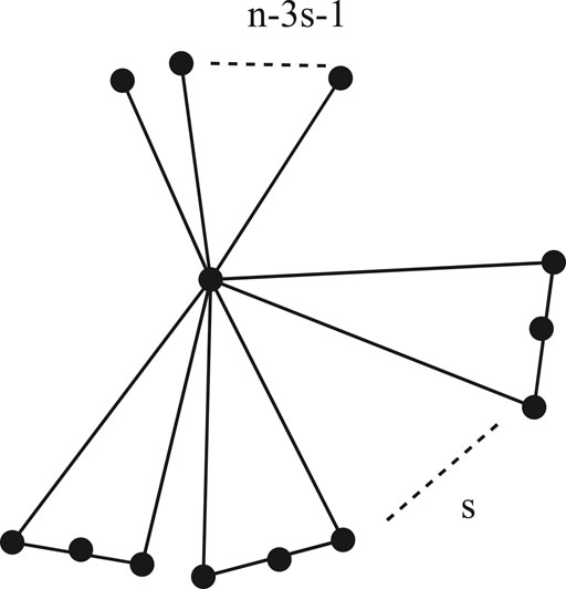
FIGURE 1. Graph
In this section, we derive the greatest value of cacti graphs for the edge Mostar invariant. First of all, some basic lemmas are proved so that the main result can be proved easily.
Proposition 2.1.(Imran et al., 2020) The edge Mostar invariant of a path
Lemma 2.1:Consider two connected graphs
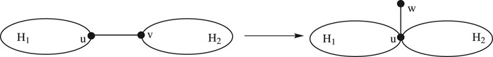
FIGURE 2. Graphs
Proof: Let
For the cut edge
Using the definition of the edge Mostar invariant and substituting the values from Eqs 3, 4 , we acquire the following:
There are two cases:
1. if
2. if
In either case, we acquire
Lemma 2.2:Let
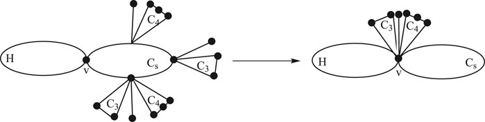
FIGURE 3. Graphs
Proof:Suppose that the vertices of
For the pendent edges
For every
1. For
2. For
3. For
1. For
2. For
3. For
1. For
2. For
3. For
4. For
5. For
6. For
7. For
Substituting the values from Eqs 5, 6 and the information from all the cases above in the definition of the edge Mostar invariant, we acquire the following:
The proof for an odd cycle
Lemma 2.3:Consider a graph H having a common vertex
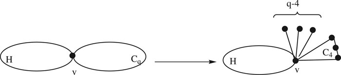
FIGURE 4. Graphs
Proof: Let H be a subgraph of
Suppose q is even; then there are three cases:
1. For
2. For
3. For
1. For
2. For
3. For
In
For
1. For
2. For
3. For
Case 1:When q is even, using the definition of the edge Mostar invariant and substituting the values from Eqs 7, 8 and the cases above, we get the following:
Case 2:When q is odd, using the definition of the edge Mostar invariant and substituting the values from Eqs 7, 8 and the cases above, we get the following:
This completes the proof. ∎
Lemma 2.4:Consider a graph H having a common vertex
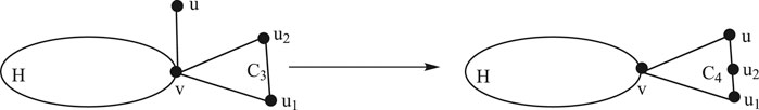
FIGURE 5. Graphs
Proof: By the construction of
There are the following cases in
1. For pendent edge
2. For
3. For
4. For
1. For
2. For
3. For
4. For
Using the definition of the edge Mostar invariant and substituting the values from cases, we get the following:
This completes the proof. ∎
Theorem 2.1: Among all the cacti graphs in
Proof: Let
Corollary 2.1. Let
equality holds if
3 Conclusion
The ongoing direction of numerical coding of the fundamental chemical structures with topological descriptors has been substantiated as completely victorious. This approach substantiates the contrast, quarry, renewal, interpretation, and swift troupe of chemical structures within enormous particularities. Eventually, topological descriptors can lead to productive measures for quantitative structure–activity relationships (QSARs) and quantitative structure–property relationships (QSPRs), which are imitations that identify chemical structures with chemical reactivity, physical properties, or biological activity. The edge Mostar index is a newly proposed quantity; it has not been used in physicochemical or biological research. Recently, a work (Imran et al., 2020) has been completed in this direction for chemical structures and nanostructures using graph operations. The authors have found the edge Mostar indices of nanostructures. Motivated by these results, we have studied the maximum edge Mostar invariant of the n-vertex cacti graphs with a fixed number of cycles in this study. For this, we have proved some lemmas in which we use the transformation of graphs and some calculations. In future, we want to find the largest and smallest edge Mostar invariants of the n-vertex cacti graphs with some fixed parameters other than the number of cycles.
Data Availability Statement
The original contributions presented in the study are included in the article/Supplementary Material; further inquiries can be directed to the corresponding author.
Author Contributions
FY: Data curation; investigation; methodology; project administration; software; validation. SA: Conceptualization; formal analysis; methodology; visualization. KA: Methodology; resources; visualization; writing-review and editing. SR: Visualization.
Conflict of Interest
The authors declare that the research was conducted in the absence of any commercial or financial relationships that could be construed as a potential conflict of interest.
The reviewer JL declared a past co authorship with the authors KA and SR to the handling editor.
References
Akhter, S., Imran, M., and Iqbal, Z. (2021). Mostar Indices of Nanostructures and Melem Chain Nanostructures. Int. J. Quan. Chem. 121, e26520. doi:10.1002/qua.26520
Akhter, S., Iqbal, Z., Aslam, A., and Gao, W. (2020). Mostar index of Graph Operations, 09416. arXiv:2005.
Akhter, S. (2019). Two Degree Distance Based Topological Indices of Chemical Trees. IEEE Access 7, 95653–95658. doi:10.1109/access.2019.2927091
Arockiaraj, M., Clement, J., and Tratnik, N. (2019). Mostar Indices of Carbon Nanostructures and Circumscribed Donut Benzenoid Systems. Int. J. Quan. Chem. 119 (24), e26043. doi:10.1002/qua.26043
Arockiaraj, M., Clement, J., Tratnik, N., Mushtaq, S., and Balasubramanian, K. (2020). Weighted Mostar Indices as Measures of Molecular Peripheral Shapes with Applications to Graphene, Graphyne and Graphdiyne Nanoribbons. SAR QSAR Environ. Res. 31 (3), 187–208. doi:10.1080/1062936x.2019.1708459
Chen, S. (2016). Cacti with the Smallest, Second Smallest, and Third Smallest Gutman index. J. Comb. Optim. 31 (1), 327–332. doi:10.1007/s10878-014-9743-z
Dehgardi, N., and Azari, M. (2020). More on Mostar index. Appl. Math. E-notes 20, 316–322. doi:10.24869/psyd.2017.39
Deng, K. C., and Li, S. (2021). Chemical Trees with Extremal Mostar index. MATCH Commun. Math. Comput. Chem. 85, 161–180. doi:10.2298/fil1919453h
Deng, K., and Li, S. (2020). Extremal Catacondensed Benzenoids with Respect to the Mostar index. J. Math. Chem. 58, 1437–1465. doi:10.1007/s10910-020-01135-0
Deng, K., and Li, S. (2021). On the Extremal Values for the Mostar index of Trees with Given Degree Sequence. Appl. Math. Comput. 390, 125598. doi:10.1016/j.amc.2020.125598
Došlić, T., Martinjak, I., Škrekovski, R., Spužević, S. T., and Zubac, I. (2018). Mostar index. J. Math. Chem. 56 (10), 2995–3013. doi:10.1007/s10910-018-0928-z
Ghorbani, M., Rahmani, S., and Eslampoor, M. J. (2020). Some New Results on Mostar index of Graphs. Iranian J. Math. Chem. 11 (1), 33–42. doi:10.21136/cpm.1987.118302
Gutman, I. (2013). Degree-based Topological Indices. Croat. Chem. Acta 86 (4), 351–361. doi:10.5562/cca2294
Hayat, F., and Zhou, B. (2019). On Cacti with Large Mostar index. Filomat 33 (15), 4865–4873. doi:10.2298/fil1915865h
Hayat, F., and Zhou, B. (2019). On Mostar index of Trees with Parameters. Filomat 33 (19), 6453–6458. doi:10.2298/fil1919453h
Huang, S., Li, S., and Zhang, M. (2020). On the Extremal Mostar Indices of Hexagonal Chains. MATCH Commun. Math. Comput. Chem. 84, 249–271. doi:10.22541/au.161825077.77699117/v1
Imran, M., Akhter, S., and Iqbal, Z. (2020). Edge Mostar index of Chemical Structures and Nanostructures Using Graph Operations. Int. J. Quan. Chem. 120 (15), e26259. doi:10.1002/qua.26259
Knor, M., Škrekovski, R., and Tepeh, A. (2015). Mathematical Aspects of Wiener index. arXiv preprint arXiv:1510.00800.
Knor, M., and Škrekovski, R. (2014). “Wiener index of Line Graphs,” in Quantitative Graph Theory: Mathematical Foundations and Applications). Editors M. Dehmer, and F. Emmert-Streib (Upper Saddle River: CRC Press), 279–301.
Li, S., Yang, H., and Zhao, Q. (2012). Sharp Bounds on Zagreb Indices of Cacti with K Pendant Vertices. Filomat 26 (6), 1189–1200. doi:10.2298/fil1206189l
Li, X., and Shi, Y. (2008). A Survey on the Randić index. MATCH Commun. Math. Comput. Chem. 59 (1), 127–156. doi:10.1063/1.5020470
Liu, H., Song, L., Xiao, Q., and Tang, Z. (2020). On Edge Mostar index of Graphs, Iran. J. Math. Chem. 11 (2), 95–106. doi:10.1155/2021/6651220
Liu, J.-B., Wang, W.-R., Zhang, Y.-M., and Pan, X.-F. (2016). On Degree Resistance Distance of Cacti. Discrete Appl. Math. 203, 217–225. doi:10.1016/j.dam.2015.09.006
Mihalić, Z., and Trinajstić, N. (1992). A Graph-Theoretical Approach to Structure-Property Relationships. J. Chem. Educ. 69, 701–712.
Randic, M. (1975). Characterization of Molecular Branching. J. Am. Chem. Soc. 97, 6609–6615. doi:10.1021/ja00856a001
Tepeh, A. (2019). Extremal Bicyclic Graphs with Respect to Mostar index. Appl. Math. Comput. 355, 319–324. doi:10.1016/j.amc.2019.03.014
Tratnik, N. (2019). Computing the Mostar index in Networks with Applications to Molecular Graphs. arxiv.org/abs/1904.04131.
Vukičević, D. (2011). Bond Additive Modeling 4. QSPR and QSAR Studies of the Variable Adriatic Indices. Croat. Chem. Acta 84 (1), 87–91. doi:10.5562/cca1666
Vukičević, D., and Gašperov, M. (2010). Bond Additive Modeling 1. Adriatic Indices. Croat. Chem. Acta 83 (3), 243–260. doi:10.5562/cca1666
Wang, C., Wang, S., and Wei, B. (2016). Cacti with Extremal PI index. Trans. Comb. 5, 1–8. doi:10.3390/math7010083
Wang, D. F., and Tan, S. W. (2015). The Maximum Hyper-Wiener index of Cacti. J. Appl. Math. Comput. 47 (1-2), 91–102. doi:10.1007/s12190-014-0763-8
Wang, H., and Kang, L. (2013). On the Harary index of Cacti. J. Appl. Math. Comput. 43 (1-2), 369–386. doi:10.1007/s12190-013-0668-y
Wang, S. (2017). On Extremal Cacti with Respect to the Szeged index. Appl. Math. Comput. 309, 85–92. doi:10.1016/j.amc.2017.03.036
Wang, S., and Wei, B. (2016). Multiplicative Zagreb Indices of Cacti. Discrete Math. Algorithm. Appl. 08, 1650040. doi:10.1142/s1793830916500403
Wiener, H. (1947). Structural Determination of Paraffin Boiling Points. J. Am. Chem. Soc. 69 (1), 17–20. doi:10.1021/ja01193a005
Keywords: topological invariants, Mostar invariant, edge Mostar invariant, cacti graphs, graph theory
Citation: Yasmeen F, Akhter S, Ali K and Rizvi STR (2021) Edge Mostar Indices of Cacti Graph With Fixed Cycles. Front. Chem. 9:693885. doi: 10.3389/fchem.2021.693885
Received: 12 April 2021; Accepted: 31 May 2021;
Published: 09 July 2021.
Edited by:
Jafar Soleymani, Tabriz University of Medical Sciences, IranCopyright © 2021 Yasmeen, Akhter, Ali and Rizvi. This is an open-access article distributed under the terms of the Creative Commons Attribution License (CC BY). The use, distribution or reproduction in other forums is permitted, provided the original author(s) and the copyright owner(s) are credited and that the original publication in this journal is cited, in accordance with accepted academic practice. No use, distribution or reproduction is permitted which does not comply with these terms.
*Correspondence: Farhana Yasmeen, farhanayasmeen.eu@gmail.com