Assessing the Local Biowaste Potential of Rural and Developed Areas Using GIS-Data and Clustering Techniques: Towards a Decision Support Tool

1 Introduction

As extreme weather events are occurring more frequently, it is of the utmost essence that the impact of anthropogenic activity on the environment is drastically reduced. The most recent Intergovernmental Panel on Climate Change (IPCC) climate report (Masson-Delmotte et al., 2021) is the last of a long list of climate reports urging countries and governments to take immediate and ambitious action to reduce their emission of greenhouse gases (GHG). Since the industrialisation, the amount of CO₂ in the atmosphere has increased with 30%. Carbon dioxide, together with methane and nitrous oxide, is one of the most important greenhouse gasses. Due to anthropogenic activity, the carbon-cycle has been unbalanced because of the additional emission of carbon dioxide into the atmosphere due the usage of fossil resources. The current additional emission amounts to 13.0 Gt of carbon every year, around 10.5 Gt of which is due to the usage and combustion of fossil fuels. Although the hydrosphere is capable of storing a lot of the additional carbon, still around 4.9 Gt of carbon remains in the atmosphere, adding to the global warming (Wöhrle, 2021).

The biosphere, i.e., the sum of all ecosystems on the planet, is just like the hydrosphere another carbon sink. Plants assimilate atmospheric carbon during photosynthesis, storing it as an energy reserve and as structural compounds in the form of biomass. Once the plants decompose, or during the plant’s respiration phase, this carbon is released back to the atmosphere. On a net level, however, the amount of carbon emitted into the atmosphere does not increase as the released carbon was initially extracted from it. This carbon cycle is the so-called short carbon cycle whereas the sequestering of carbon in rocks (and fossils) is denominated the long carbon cycle.

As biomass is the largest non-fossil carbon source on the planet and has compelling advantages over fossil carbon, it is coined as the best candidate for replacing fossil fuels and fossil raw feedstocks all together. Public opinion on the employment of more sustainable and renewable processing practices in the chemical and energy sector has in the past decades taken a significant step in its favour. However, both industries are still heavily dependent on (fossil) carbon, both as a feedstock and as an energy source. Reducing the carbon footprint of these industries will be a considerable challenge. Unsurprisingly, reducing the climate impact of these sectors has gradually become more and more a major point of discussion on international fora. During the 2020 World Economic Forum meeting in Davos, one of the discussions focussed on how to build a more climate-friendly chemical industry (Brudermüller, 2020). It was indicated that one of the corner stones of reducing the carbon footprint of the chemical industry, will be to use carbon more efficiently. A so-called multi-pronged approach was proposed, based on three main pillars: 1) process and energy optimisation, 2) renewable energy supply, and 3) CO₂ reduced breakthrough technologies (Brudermüller, 2020). Similarly, Boulamanti and Moya (2017) indicate that biomass is a potential feedstock to replace petroleum resources.

However, to unlock the potential of lignocellulosic biomass (i.e., the type of biomass and/or biowaste considered in this contribution), it must be processed first. The conversion of biomass to useable and valuable products is done using biorefinery processes. Depending on the feedstock used, i.e., its physico-chemical properties, different processes are employed to disrupt the crystalline lignocellulosic biomass structure and convert the obtained intermediates in finished products or platform chemicals. Whereas finished products, like bioethanol and -gas, can be immediately marketed, platform chemicals need to be processed further.

Cherubini et al. (2009) introduced a general classification system for biorefineries based on the type of platforms, feedstock, and processes they use and the products they produce. Generally, four biorefinery generations can be distinguished. First generation biorefineries were developed as an alternative for petroleum refineries, mostly producing liquid biofuels and energy from uniform food crops (Naik et al., 2010). While the usage of food crops and arable land for the production of energy was deemed to be morally skewed, research efforts have now shifted towards a second generation of biorefineries that use non-food and biowaste as their feedstock (Carroll and Sommerville, 2009; Isikgor and Becer, 2015; Jeevahan et al., 2021). Third generation biorefineries employ algae and other microbial cell factories for the production of energy and chemicals, whereas fourth generation biorefineries use genetically modified organisms as a feedstock (Cherubini et al., 2009; De Buck et al., 2020).

As early generation biorefineries were mostly designed as an alternative for petroleum refineries in a context of unstable and relatively high oil prices, they were not necessarily designed to have a low impact on the environment from an operational point of view. They mainly relied on the economy-of-scale to become economically sustainable and competitive with regard to their petroleum-based counterparts (Naik et al., 2010; Mohr and Raman, 2013). Hence, they require a large and steady stream of a uniform feedstock, which is often either a food crop or an energy crop grown on arable land that can, therefore, no longer be used for growing food. Even though the disadvantages of large-scale mono-feedstock biorefineries are becoming more obvious (Leong et al., 2021), the implementation of the far more sustainable small-scale flexible-feed biorefinery is still lagging behind (Bruins and Sanders, 2012; Kolfschoten et al., 2014; Álvarez del Castillo-Romo et al., 2018). To bridge this gap, the proposed decision support tool (of which the bio-inventory tool presented in this contribution will be a part of) will focus on the design of a small-scale second generation biorefinery which is optimally embedded in its local setting.

One of the main issues regarding small-scale flexible-feed biorefineries is the uncertainty operators face with regard to the feedstock stream (Elia and Floudas, 2014; Wang et al., 2015; Schröder et al., 2018). When designing a biorefinery, it is of the essence to have a good overview of which feedstocks are locally available and in which amounts. Based on this knowledge, an optimal biorefinery could be designed that is specifically tailored to process these local biowaste streams and produce locally desired products. A more detailed discussion on the general aspects of designing a (locally embedded) biorefinery, as well as on previous work with regard to modelling biorefinery supply chains and estimating the biomass/biowaste potential of a certain area, is included in Section 2.

The design of an optimally locally embedded biorefinery requires in-depth knowledge and insight on the three main aspects of a biorefinery system, i.e., the feedstock, the (conversion) processes, and the products (see also Section 2). Therefore, a decision support tool (DST) is being developed for designing and optimising an optimal locally embedded small-scale biorefinery. Figure 1 displays the outline of the DST that is being developed. This paper presents the first building block of the DST: the bio-inventory tool.

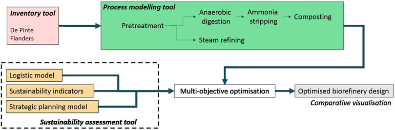
FIGURE 1. Outline of the proposed decision support tool. This paper focusses on the inventory tool.

As introduced above, one of the most important aspects of a well-designed biorefinery is the usage of a locally available feedstock. The types of feedstocks that are available, as well as their estimated annual yield, will have a big influence on how the biorefinery is designed as they influence the choice of processes suited for the conversion step and, thus, the products that can be expected. The bio-inventory tool will allow decision makers (DM) to assess which feedstocks are locally available and in which quantities and/or quality. This paper especially focusses on developing a general inventory approach, valid for the region of Flanders in Belgium and with the potential to be extended further. Two different approaches are presented: 1) A colour clustering method, based on the ground cover maps available for Flanders, and 2) a clustering method based on residential centres, ribbon development, rural, and industrial buildings. The information generated by the bio-inventory tool will be subsequently used by the process modelling tool and the optimisation tool to draft an optimal biorefinery lay-out (Figure 1). The final decision support tool is being developed as an online tool and will be made available as soon as all building blocks have been developed and are connected.

This paper is structured as follows: in Section 2, the overall small-scale biorefinery design strategy employed in this paper is presented. In Section 3, the employed materials and methods are presented. Section 4 focusses on presenting two novel biowaste quantification approaches employed in the bio-inventory toolbox. In Section 5, both quantification methods are applied to a case study region. Finally, the extendibility of the proposed methods is discussed in Section 6, and Section 7 summarises the main conclusions of this paper.

2 Designing Small-Scale Locally Embedded Biowaste Biorefineries

2.1 Small-Scale Biorefineries

As mentioned in the introduction, small-scale locally embedded biowaste biorefineries are a specific type of biorefinery designed to amend several disadvantages of early generation biorefineries. The latter were developed as alternatives for petroleum refineries, not necessarily out of environmental consideration, but rather due to volatile oil prices and uncertain supply chains (Mohr and Raman, 2013). While most countries do not posses their own oil natural resources, they are reliant on a few oil-producing countries, resulting in a heavy dependency, unstable and relatively elevated oil prices. To obtain a higher level of energy independence, alternative ways were sought to produce (liquid) fuels and platform chemicals without a need for raw oil. Large-scale sugar and starch processing biorefineries were developed to achieve this goal. They heavily rely on a high throughput of a uniform feedstock and economy of scale, and produce (a high amount of) low value-added products like biofuels and bulk chemicals. However, as these types of biorefineries directly compete with cheap petroleum-based products, their economic striking power is rather limited (Naik et al., 2010).

While large-scale biorefineries were designed using a very similar pattern like conventional petroleum refineries (or as a replacement for the latter, more specifically) (Mohr and Raman, 2013), small-scale biorefineries (SSBR) resolutely left these practices behind (Bruins and Sanders, 2012; Ait Sair et al., 2021). Instead of competing with petroleum refineries for the production of fuels and bulk chemicals, small-scale biorefineries focus on the production of high value-added products, using locally available biowaste streams, that are highly desired in a certain region. Although the economy of scale is lost in these designs, they can still outperform large-scale biorefineries given that they employ an integrated design (Bruins and Sanders, 2012; Clauser et al., 2016; De Visser and Van Ree, 2016).

Integrated biorefineries are designed in such a way that the amount of waste streams leaving the plant are minimised (Tay et al., 2011; Geraili et al., 2014). In practice, this means that every biomass stream of the biorefinery is maximally utilised and valorised. An additional advantage of small-scale biorefineries which process local (plant-based) biowaste is the fact that, in essence, they function as local waste-processing facilities (Leong et al., 2021). Especially when considering (peri-)urban areas, where the biowaste potential with regard to municipal and private (plant-based) biowaste is elevated, decentralised waste-processing facilities could contribute greatly to strengthening the local circular bio-economy (Thiriet et al., 2020; Glivin et al., 2021; Angouria-Tsorochidou et al., 2022). However, when designing such biorefinery systems, it is of the essence that the local biowaste potential is well-known, as its suitability to its geographical context is crucial with regard to its economic and environmental sustainability (Angouria-Tsorochidou et al., 2021).

As the symbiosis between the local context of the biorefinery, the conversion processes used (and how they are operated), and the products produced is too complex to be considered as such, decision makers must rely on in silico tools to support their planning and designing efforts.

2.2 A Decision Support Tool for Designing a Small-Scale Biorefinery

Thanks to their decreased size, small-scale biorefineries are significantly more inexpensive than their large-scale counterparts, rendering them an attainable option for communities, farms, and other, less financially powerful, interested parties. Nonetheless, as the biowaste feedstocks these facilities require are inherently accompanied with many uncertainties (Geraili et al., 2016), nor are the processes they employ yet widely implemented (Jeevahan et al., 2021). An (online) decision support tool can bridge this gap in knowledge potential biorefinery investors are facing by providing an in-depth in silico assessment of the biorefinery’s potential performance and suitability for its local setting at the early stage of biorefinery design.

The biowaste potential assessment approaches presented in this contribution make up the first tool (the bio-inventory tool) of an online decision support tool for designing and optimising a local, small-scale biorefinery. Figure 1 represents the ultimate foreseen outline of the decision support tool. Starting from the bio-inventory toolbox, the feedstocks available in a local setting will be identified and quantified. Employing two methods, as presented in this paper, the bio-inventory tool will enable the decision makers to assess which feedstocks are locally available and in which quantities. The assessment of the biowaste potential (and, thus, the biowaste biorefinery potential) of a certain area, is a first and crucial step towards designing a sustainable biorefinery system.

Subsequently, the obtained knowledge from the bio-inventory toolbox will be sent to the process toolbox where, based on a multitude of (sustainability) indicators, optimal biorefinery layouts will be designed, all tailored for the feedstocks that are available in the defined catchment area. A process framework has been designed, based on expert knowledge, and will be used as the initial modelling framework for the BR (Sbarciog et al., 2022). Depending on the properties of the defined catchment area, certain conversion processes will become more or less suitable for processing the selected biorefinery feedstock.

Because of the inherent diffuse nature of biowaste, any given catchment area will mostly contain multiple biowaste feedstocks. Consequently, multiple BR designs could be drafted for one certain catchment area. In order to aid the decision maker to select one design for further investigation and, potentially, implementation, the final step of the proposed DST consists of comparing all the designs with each other, employing comparative visualisation techniques. Based on this, the decision and/or policy maker will eventually be able to select a certain design.

2.2.1 Strategic Planning of a Biorefinery

A biorefinery system can be divided into three main parts: 1) the feedstock part, 2) the process part, and 3) the product part. Each part is defined by its own set of strategic decisions (Figure 2). Depending on the available local facilities and/or needs, a biorefinery can be designed starting from any part. However, as all three parts are dependent on each other, it is crucial to know how decisions made with regard to a certain part influence the freedom of choice of the remaining strategic decisions with regard to the other two parts. E.g., when a certain process is selected as a conversion process for the biorefinery plant, the choice of feedstocks that can be processed with this specific technology will be constrained and, simultaneously, the products the biorefinery will be able to produce for the (local) market are too. Therefore, when designing an integrated biorefinery that is optimally embedded in its local setting, it is essential to know the rippling effect, i.e., the influence certain decisions have on others.

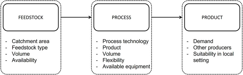
FIGURE 2. Flowsheet representing the three biorefinery design entry points and their accompanying main strategic design decisions.

For this purpose, initial steps towards a strategic planning model are taken, which will be incorporated in the decision support tool. A strategic planning model (SPM) is defined as a set of interdependent present and future decisions and their reciprocal links (Radford, 1979). The SPM provides a framework for taking strategic decisions that have a big influence on how, e.g., a biorefinery plant is run and, thus, its (economic) viability. Often, these decisions have major rippling effects, meaning that they heavily affect the outcome of other decisions and/or limit the decision options available. As their outcomes are often not easily reversible, they need to be taken after thorough deliberation. Amongst others, Sharma et al. (2011) and Geraili et al. (2016) have developed tools for aiding decision makers in designing a biorefinery whilst simultaneously taking strategic considerations into account. Sharma et al. (2011) have proposed a design and optimisation framework for a biorefinery which is: 1) economically sustainable by creating value, 2) environmentally sustainable when considering greenhouse gas (GHG) emissions and waste streams, and 3) socially sustainable by minimising its (negative) impact on the local community. Geraili et al. (2016) consider the uncertainty that accompanies the strategic and operational decisions. Knowing this, as well as how these uncertainties propagate to other decisions, is essential when designing a biorefinery system. Therefore, one of the main targets of a strategic planning model is to estimate how a certain decision influences other decisions, and what its effect will be on the long term.

Within the presented design and optimisation framework, at each step of the designing process, the tool will provide the DM with a set of options for each strategic decision that needs to be made whilst simultaneously showcasing how decisions influence one another and additionally suggesting, if necessary, more economically viable and sustainable alternatives. Eventually, users will be able to compare their foreseen design with designs proposed by the tool, using a multitude of indicators.

Figure 3 represents the biorefinery designing process starting from the feedstock part and gives an overview of the order of strategic decisions that need to be taken, as well as how they influence each other. Strategic decisions that can be attributed to the feedstock entry point include the catchment area, i.e., the area from which feedstocks will be harvested. Choosing this catchment area will already constrain a horde of other strategic decisions as it (potentially) limits the feedstock types that will be available, their volumes, and, depending on local competition for a certain feedstock, their availability. These designing aspects limit, on their turn, the freedom of choice with regard to strategic decisions at both the process and product entry points. In general, as the rippling effect of decisions made at the feedstock entry point is the biggest of all three designing entry points, it is deemed that ostentatiously starting the designing exercise from this entry point is a reasonable modelling simplification. As the ultimate goal of the decision support tool is to support decision and policy makers in assessing the viability of a biorefinery design in their own local setting, this entry point will also be the most likely one to be selected, as both often start from assessing what is possible in a certain catchment area of interest. Only when there is already dedicated equipment available, or when a certain biorefinery product is especially desirable in a local area, the other two designing entry points could be considered.

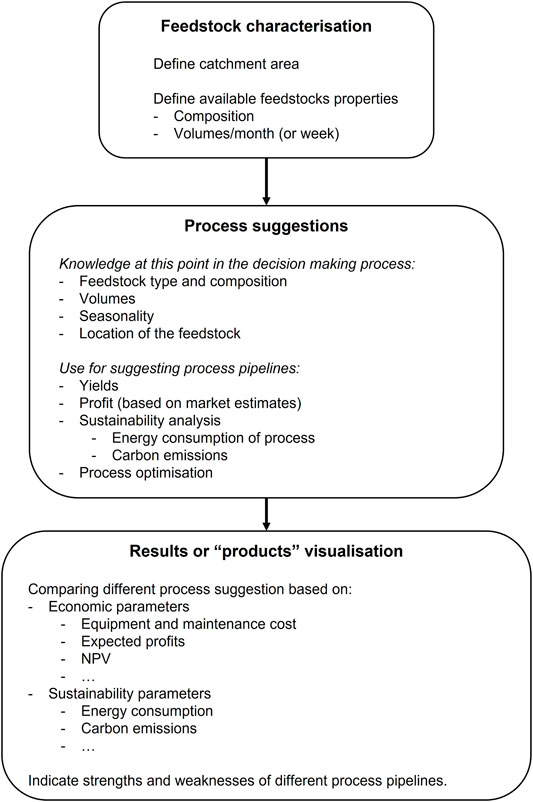
FIGURE 3. Flowsheet representing the biorefinery designing process and the accompanying strategic decisions, starting from the feedstock entry point.

2.2.2 Modelling the Local Setting of a Biorefinery

When designing an integrated small-scale biorefinery, the employed conversion processes must be optimally coordinated to the feedstock that is processed: the biorefinery should be optimised for their local setting. However, in order to be able to do so, this requires a thorough knowledge of the locally available waste streams, their amounts, and their seasonality and harvest times. As displayed in Figure 3, the properties of the feedstock that is to be processed, has major influences on which conversion processes are available and, consequently, which products can be produced. Accordingly, a thorough and reliable estimation and/or model of the local setting of the SSBR (i.e., its supply area), is an essential first step in the design process.

The modelling and performance analysis of biorefinery supply chains has been considered in a multitude of previous works. Especially while their overall implementation is still limited, most supply chain modelling efforts and/or decision support tools focus on meeting the lack of commercial experience most biorefinery set-ups are facing, both with regard to their supply chains and the conversion technologies they use. Wang et al. (2015) have, for instance, produced mathematical models to estimate the production of energy crops by modelling their growth kinetics, whereas Elia and Floudas (2014) provided a thorough review of supply chain optimisation and the usage of hybrid feedstocks. They coined that hybrid processes, which can process a multitude of different feedstocks, provide their exploiters with synergetic advantages in the sense of reducing costs and/or increasing feedstock security. Note that they mostly discussed the hybridisation of fossil and biomass-based feedstocks, whereas this paper focusses on modelling supply chains for small-scale flexible feed biorefineries that can process a multitude of lignocellulosic biomass-based feedstocks. Combined with optimising supply chains comes the issue with regard to siting the biorefinery, which was considered in the work of Schröder et al. (2018) and Martinkus et al. (2019). Lemire et al. (2019) employed GIS-data to analyse how a decentralised supply chain and biorefinery system, as coined in this contribution as well, compares to a centralised system, ascribing an increased efficiency to the former. Note that the biorefinery siting will not be considered in the supply chain modelling presented in this paper. Schröder and Geldermann (2019) additionally presented a generic method on how to employ spatial data obtained from GIS-datasets for the quantification of geo-spatially spread biomass. On a more holistic level, Sukumara et al. (2014), developed a decision support tool for assessing different biorefinery technologies by simultaneously considering the performance and economic viability of the (required) supply chains and, by doing so, taking first steps towards an overall sustainable biorefinery designing process. Lastly, Junqueira et al. (2016) presented the major strength of decision support tools in the context of supporting the formulation of novel and ambitious policies in view of making the energy sector more sustainable. Virtual biorefineries, as coined by Junqueira et al. (2016), can fill the gap that is left by the few real-life implementations of these technologies to increase investors’ trust in the considered technologies.

As mentioned before, the biowaste potential assessment approaches presented in this paper will be part of a more thorough decision support tool, whose main goal will also be to provide decision and policy makers with an easy and low-entry method to assess the overall sustainability of a potential biorefinery design in a local setting.

3 Materials and Methods

3.1 GIS-Datasets

The case study region of this contribution is Flanders, and more specifically the commune of De Pinte in the province of Eastern-Flanders. Therefore, the presented GIS-datasets all focus on this particular area.

3.1.1 Ground Cover Map

The colour clustering method proposed in this paper employs the Bodembedekkingskaart (BBK), 1m resolutie, opname 2015 (Agentschap Informatie Vlaanderen, 2019) (hereafter referred to as ground cover map). Figure 4 represents an excerpt of this ground cover map of the Flanders region, Belgium. Every type of ground cover, i.e., buildings, vegetation, watercourses, etc., is represented in a different colour depending on its usage and/or properties. The ground cover map provides a surface area-based categorisation of different geographical locations, with a resolution of 1 m². The colour clustering method will enable users to calculate the total surface area belonging to certain ground cover and/or usage. This information can be further used to make a surface area-based assessment of the expected amounts of biomass and/or biowaste coming from this particular ground cover category. The colour clustering method is explained more in detail in Section 4.1.

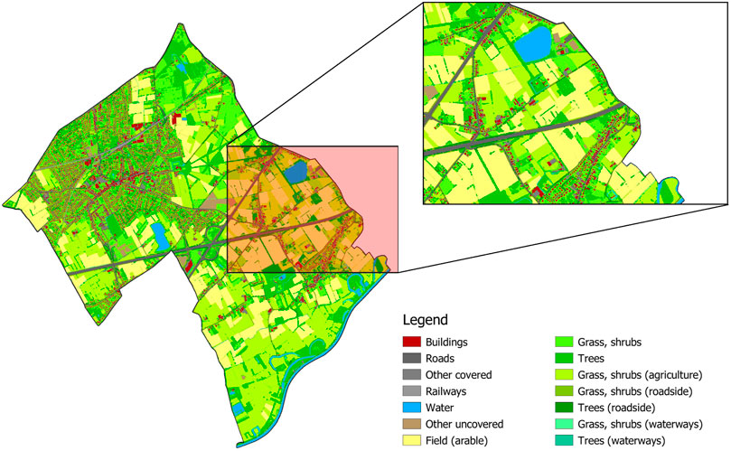
FIGURE 4. Ground cover map.

3.1.2 Buildings’ Register and Residential and Ribbon Clusters

The building clustering method, presented in Section 4.2, does not employ a surface-based quantification approach but instead allocates periodic biowaste yields to discrete points on a map. More specifically, the used Gebouwen- en Adressenregister (Agentschap Informatie Vlaanderen, 2021) (hereafter referred to as buildings’ register) provides a dataset containing all the building units in Flanders (i.e., one data point per building unit). Every data point contains information about, i. a. the building unit’s state (i.e., historical, realised, or planned) and it is geographical location. Every building unit (or data point) is characterised by a unique ID, which will be used in the building clustering method to allocate additional data to a selection of data points or building units. Figure 5 visually represents an excerpt of this dataset.

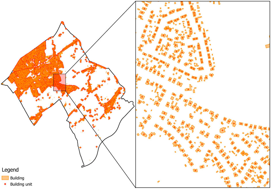
FIGURE 5. Buildings’ register.

Next to densely built-up clusters of housing (e.g.: village or city centres) and rural building, Flanders is known for a third type of development: the, so-called, ribbon development. As all three categories of building development are relatively different from each other, it is important to know to which development type a building belongs. To achieve this, an additional dataset, i.e., Kernen, linten, verspreide bebouwing in Vlaanderen (Vlaamse Overheid - Departement Omgeving - Afdeling Vlaams Planbureau voor Omgeving, 2013b) (hereafter referred to as Cluster and ribbon database), is used as a filter for categorising all the building units in the case study area to their according development type. In Figure 6, a visual fragment of this dataset is presented.

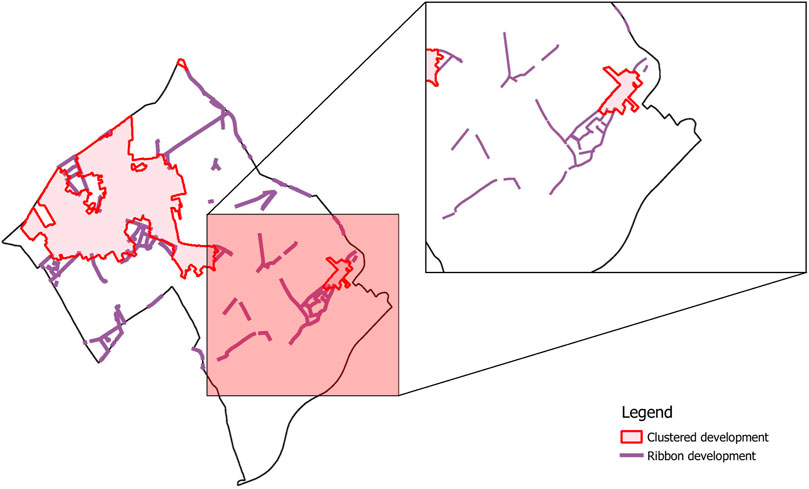
FIGURE 6. Clustered and ribbon development in the case study region.

3.2 Software

The GIS-datasets were handled and manipulated using QGIS 3.10 (QGIS Development Team, 2021) on a 64-bit Windows 10 system with an Intel Core i5-8500 CPU @ 3.00 GHz processor and 16 GB of RAM installed. The colour clustering method was developed in Python 3.9.6, using the k-means clustering method of the sci-kit learn Python module (Pedregosa et al., 2011).

4 Results and Discussion

In order to link quantitative data about biowaste availability and composition to geographic locations, two methods are proposed: 1) The colour clustering method, which employs the ground cover map, and 2) The building type clustering method, which uses the buildings’ register. Whereas the first method employs a surface area based method for assessing the amounts of biowaste that can be anticipated in an area, the second method is based on allocating anticipated biowaste amounts to discrete points on the map. Combining these two methods will allow users of the small-scale biorefinery decision support tool to draw the borders of their foreseen collection area and calculate the locally available biowaste types and quantities.

4.1 Colour Clustering Method

The first biowaste quantification method focusses on agricultural biowaste and employs an area-based quantification approach. Based on the boundaries of the collection area, the ground cover map of this area is retrieved and processed, resulting in area-based estimations of the yields of agricultural waste streams. The two types of agricultural waste streams that will be quantified using this technique are stover and/or straw obtained from the cultivation of cereals and grains, and grass cuttings and/or silage obtained from the maintenance of agricultural grasslands.

4.1.1 Quantifying Colours in a Figure

The ground cover map is made up out of 14 different colours, each representing a different ground coverage and/or usage. Table 1 summarises all the colours with their RGB-code and the coverage or usage they represent. The clustering method uses a k-means clustering method to cluster all the pixels of a selected part of the ground cover map into 14 different colour clusters. The ratio of pixels attributed to a certain colour clusters is equal to the relative total occurrence of the ground cover that can be linked to that colour as the total surface of the selected area is known.

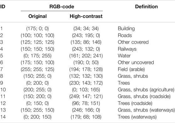
TABLE 1. Summary of the colours of the ground cover map.

The ground cover map is largely based on aerial photos, obtained during the summer of 2015 (Agentschap Informatie Vlaanderen, 2019). Due to the fact that high and low ground coverages overlap, e.g., trees and roads, their corresponding colours on the ground cover map overlap too (Figure 7). Due to these overlapping colours, the ground cover map counts more unique colours than the 14 colours that are listed and linked to a certain ground cover type. Therefore, quantifying the relative occurrence of each colour by simply counting the number of pixels with the corresponding RGB-code was not a feasible quantification technique. To illustrate this, the ground cover map image displayed in Figure 7 has a width of 2,661 pixels and a height of 1867 pixels and covers an area of 0.427 km². For this particular example, each pixel of the image represents an area of 0.086 m², which is more than ten times smaller than the resolution of the ground cover map itself. As the zoom level of a map-image will influence the eventual resolution of the map and, therefore, the colours that are showcased, it is essential to keep the area represented by one pixel smaller or, in the worst-case, equal to the resolution of the ground cover map itself. However, even when the area represented by one pixel is more than ten times smaller than the resolution of the ground cover map, the image still counts 178 unique colours.

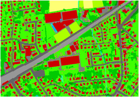
FIGURE 7. Zoomed in snippet of the ground cover, clearly displaying overlapping colours (area = 0.427 km²).

Data analysis allows for extracting useful information from a dataset. More specifically, the set of pixels, and their corresponding RGB-codes, representing an area of interest could be clustered in x clusters using data analysis techniques. The clustering technique selected for this, is the k-means clustering method. The k-means clustering method allocates n elements to k clusters, with k ≤ n, by minimising the squared Euclidean distance between all elements in a cluster k_i and their mean value μ_i:

with K = {K₁, K₂, … , K_k} the set of clusters. The k-means clustering method was deemed the most suitable for the task at hand as it clusters elements based on their distance to the cluster centres. In the context of clustering pixels of an image in k clusters, each element n is made up out of three features x_i, i.e., its corresponding RGB-code. Figure 8 displays the location of the unique colours of the snippet displayed in Figure 7 versus the location of the colours that correspond with a certain ground cover type. It can be seen that for this sample, the unique colours are either mostly already clustered around a colour that was listed in the legend or are located on the connecting line between two listed colours as they are a linear combination of both. Both observations further substantiate the selection of the k-means clustering method. As most unique colours are located in the proximity of listed colours, the clusters centres that are defined by the k-means clustering method will, most likely, be located in the vicinity of the centres of these already existing clusters. Furthermore, unique colours located on the connecting line between two listed colours will most likely be attributed to either of the corresponding clusters. As those unique colours represent an overlap of both of these listed colours, they can be attributed to either one. The colour clustering method is presented in Algorithm 1.

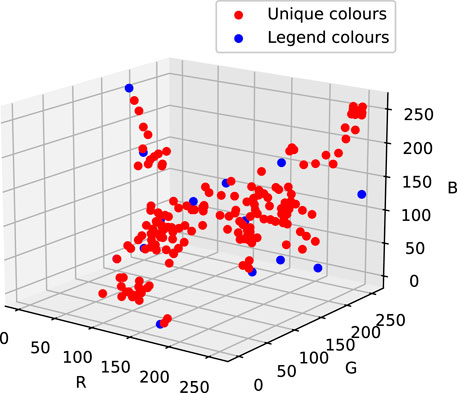
FIGURE 8. Unique colours (red) vs listed colours in the legend (blue).

Algorithm 1. Colour clustering algorithm

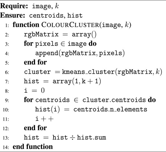
The colour clustering algorithm starts with storing all the RGB-codes of the pixels making up the image of the ground cover map representing the area of interest. This list of w × h vectors (with w the width of the image and h the height in pixels) is clustered into k clusters. Each vector has a dimension of (1 × 3), or, is made up out of 3 features. Subsequently, a normalised histogram is drafted to quantify the number of pixels that are attributed to each cluster. The ratio of pixels attributed to a certain cluster, which can on its turn be linked to a certain ground cover, is equal to the ratio of surface area that is covered with this particular ground cover in the studied region.k is set to 14, by default, as the ground cover map links, in theory, 14 unique colours to a certain ground cover. However, initial results of random snippets of the ground cover map show that the colour clustering method struggles to distinguish between the different grey colours, used to indicate roads, railways, and other covered areas, and the colours resulting from overlapping ground coverages. A first remediation trial was to decrease the number of clusters, k, to 13, 12, and 11. The results of this approach are presented in Figure 9.From (Figures 9B–E), it can be seen that by reducing the number of clusters, the most prominent colours of the ground cover map are more accurately approximated by the clustering method than when using a higher number. In order to verify this observation, the inertia of each clustering process was calculated. The inertia is a measure for assessing how accurately a set of data points is clustered by the k-means clustering method by calculating the spread of data points within each cluster [see Eqs (2, 3)]:

with

and m the number of data points x assigned to a cluster n, defined by a centroid μ_n.By calculating the overall inertia for a different number of clusters, the most optimal number of clusters can be defined using the elbow method. As the overall inertia will inevitably decrease with an increasing number of clusters k, the most optimal number of clusters corresponds with the lowest k that simultaneously displays a low overall inertia. When looking at the evolution of the inertia of the clustering method (Figure 9F), it can be seen that this so-called elbow corresponds with a number of clusters higher than 14. Nonetheless, even though a higher number of clusters would more accurately represent the trends of the data set (including the additional, non-listed, colours obtained from overlapping), the number of clusters k is kept at 14 since only 14 different types of ground coverage have been defined. Using a higher number of clusters would result in more cluster centres than listed colours, i.e., multiple cluster centres will have to be assigned to one listed colour or ground cover type. Due to the high level of overlapping colours (or noise on the data), using a higher number of clusters would result in an increased influence of this noise on the clustering performance and, therefore, a decrease in the accuracy of the estimation of the (prominent) cluster centres.Another remediation approach was to seed the k-means clustering algorithm with the RGB-codes of the original, listed colours. In Figure 10 it is visible that the clusters eventually defined by the algorithm are not identical to those that were seeded. The downside of this approach is that the algorithm only initialises the clustering procedure once, i.e., with the seeded set of listed colours. Nonetheless, as can be seen in Figure 10, seeding the k-means clustering algorithm with RGB-codes of the original, listed colours resulted in a better clustering effort than without seeding. Especially the different types of so-called covered areas (i.e., roads, railways, and other covered areas) are more accurately approximated by the clusters’ centroids.Finally, the third remediation approach to improve the clustering method’s accuracy was to replace the colours of the ground cover map with a set of 14 colours from the list of most contrasting colours as presented by Kelly and Judd (1976); Green-Armytage (2010). The colours of the original ground cover map are namely chosen in such a way that the link between the used colour and the ground cover it represents, is intuitive. E.g., green vegetation, like grass and trees, are represented using green colours (see colours 7 to 14 in Table 1 and Figure 4). However, for the purpose at hand, the intuitive link between the colour and the ground cover it is representing is subordinate to the ease of clustering them in k clusters. Figure 11 displays the same snippet of the ground cover map, once in the original colours, and once in the highly contrasting colours, and the obtained centroids for k equal to 14, once with 10 random initialisations, and once with seeding the 14 original/highly-contrasting colours (Table 1). The ground cover map snippet with the original colour scheme counts 176 unique colours whereas the high-contrasting one counts 212 unique colours. Nevertheless, both the seeded and unseeded clustering efforts of the ground cover map with highly contrasting colours displayed an overall inertia of 2.0 10⁹, compared to overall inertias of 3.5 10⁹ and 3.2 10⁹, respectively, for the clustering efforts of the ground cover map using the original colour scheme. Additionally, in Figure 11G, it can be seen that the inertia of the clustering performed by the k-means algorithm on the ground cover map snippet employing the highly contrasting colours, is consistently lower than those using the original colours, indicating an overall improved clustering performance. Therefore, as the method using the highly contrasting colours clearly displays a significant decrease in inertia for the same clustering exercise, independent whether or not the used colours’ RGB-codes were seeded, this method will be used when applied to the case study.

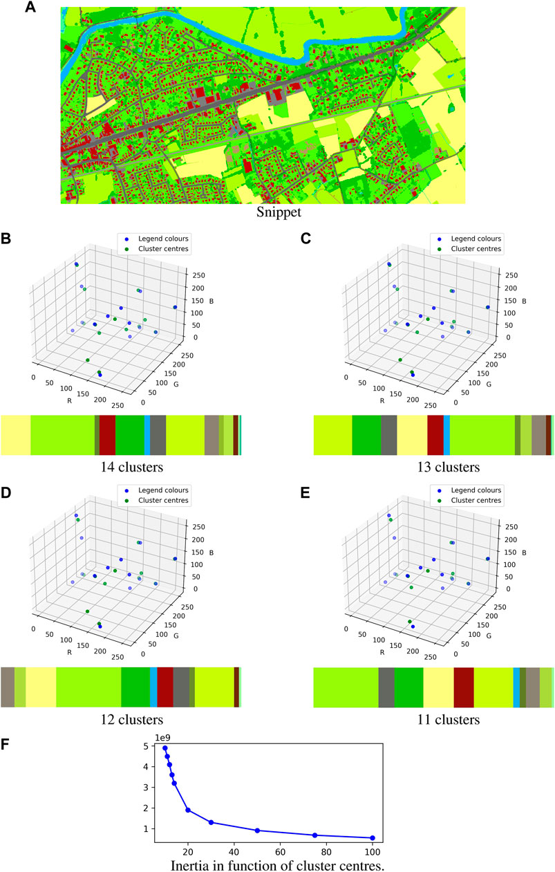
FIGURE 9. Effect of cluster reduction. (A) Snippet, (B) 14 clusters, (C) 13 clusters, (D) 12 clusters, (E) 11 clusters, (F) inertia in function of cluster centres.

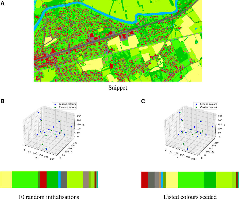
FIGURE 10. Effect of seeding the original colour centres. (A) Snippet, (B) 10 random initialisations, (C) Listed colours seeded.

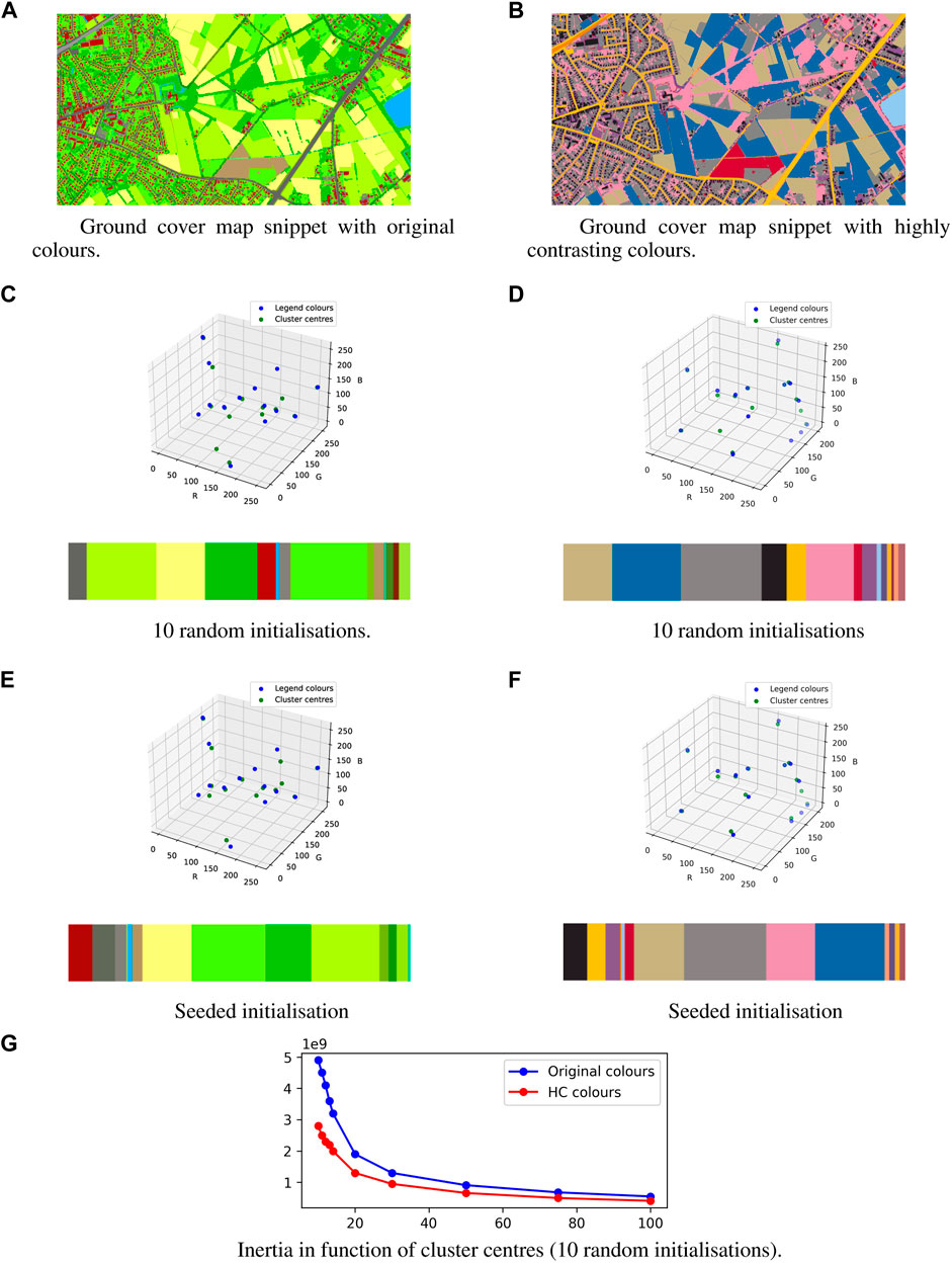
FIGURE 11. Effect of the employment of highly contrasting colours on the colour clustering method using the k-means. (A) Ground cover map snippet with original colours, (B) Ground cover map snippet with highly contrasting colour (C) 10 random initialisations (D) 10 random initialisations (E) Seeded initialisation (F) Seeded initialisation (G) Inertia in function of cluster centres (10 random initialisations).

4.1.2 Area-Based Biowaste Quantification

The presented colour clustering approach is especially useful for quantifying biowaste-streams that are sporadically harvested and which volumes are influenced by the surface area that is harvested. Specifically agricultural waste, like grass cuttings, silage, corn stover, and wheat straw, are easily quantifiable using a surface area-based technique.

Regarding surface area-based yields for grass cuttings, Van Meerbeek et al. (2015) assessed the biowaste yields obtained from the maintenance of conservation areas and roadsides in Flanders, Belgium. It is assumed that the grass cuttings obtained from agricultural land in Flanders are most alike to the grass cuttings obtained from roadside maintenance. Van Meerbeek et al. (2015) obtained a value of 4.48 ± 1.59 ton DM/ha per mowing cycle. At this stage of the decision support tool, only one mowing cycle is taken into account. In a later development stage, it would be desirable to allow users to interact more with the tool, especially at the level of characterising their local conditions. Note that when two or more mowing cycles are considered, biomass re-growth needs to be considered too (De Meyer et al., 2016).

When considering the surface-area based yields of straws and stover obtained from the cultivation of cereals and grains, like corn, wheat, barley, oats and rye, a further simplification has to be made. As the database of the ground cover map (Agentschap Informatie Vlaanderen, 2019) does not provide sufficient detail to assess which types of cereals and/or grains are grown on arable land, additional information is required on the occurrence of certain cereals and grain crops in Flanders, Belgium. Using the information provided by the Landbouwgebruikspercelen LV, 2020 database Vlaamse Overheid - Departement Landbouw en Visserij (2020) (hereafter referred to as the agricultural usage database), it is first assessed how much of the total arable land in Flanders is used for the tillage of grains and cereals. Subsequently, as the agricultural usage database additionally provides information on which crop is grown on a certain plot of arable land in Flanders, the ratio of the five major grains grown in Flanders (i.e., corn, wheat, barley, oats, and rye) is determined. The Food and Agriculture Organization of the United Nations (FAO) reported that in 2017, Belgium produced 9.05 ton DM/ha of cereals and grains (Food and Agriculture Organization of the United Nations, 2020). In that same year, 48.58% of arable land in Flanders was used for the cultivation of corn, 16.87% for the cultivation of wheat, 4.46% for the cultivation of barley, 0.12% for the cultivation of oats, and 0.09% for the cultivation of rye. Renard et al. (1997) reported for these crops a residue to harvest ratio of 1.00, 1.50 (average between winter and summer wheat), 2.00, 2.00, and 1.50 kg residue/kg DM harvested, respectively. The weighted average residue to harvest of grains for Flanders, based on the ratio of arable land used for cultivating a particular grain, equals 6.35 ton DM/ha. Applying the same weight ratio for calculating the weighted average residue yield per ton DM harvest, renders 1.18 ton residue/ton DM harvested. Combining the weighted yield of cereals and grains in Flanders with the weighted residue yield renders a weighted average residue yield of 7.49 ton residue/ha of arable land.

The proposed colour clustering method, together with the surface-area based biowaste quantification approach presented above has been applied to quantify the yearly to-be-expected volumes of agricultural biowaste in the region of De Pinte, Belgium (see Section 5).

4.2 Building Unit Clustering Method

Whereas the first quantification method mainly focussed on agricultural waste and presented a surface area-based approach to assess the amounts of biowaste that can be expected in a local area, the building unit clustering method employs scattered data points on the map. More specifically, each data point represents one building unit. A building unit is defined as (Agentschap Informatie Vlaanderen, 2021):

“(a building unit is) The smallest unit within a building that is suited for residential, commercial, or recreational purposes, that is accessed via a private lockable entrance from the public road, a yard, or a shared circulation space. The unit is independent from a functional point of view. Additionally, a building unit can be a common part.”

In essence, every building unit can be considered as a production site of kitchen and/or garden waste. In the studied case study region, this particular type of waste is collected biweekly via door-to-door collection. Therefore, while the agricultural waste, that was considered in the colour clustering method, is only harvested once a year, the kitchen waste provides a much more steady flow of biowaste that is readily available and cheap to obtain.

The major challenge of this approach, however, comes with the fact that correlation between the amounts of biowaste produced per building unit is depended on the number of people living in or using the unit in question. Especially when looking at densely populated city centres, it becomes obvious that there is no one-to-one relationship between the number of building units present in a certain area versus the amount of people occupying them. Based on the definition given above, for example, high rise apartment buildings are also only one building unit even though they house multiple households. For the sake of simplicity, it is assumed that, on average, households of the same size generate the same amount of kitchen waste, regardless of whether they live in a single family home or in an apartment building or another type of shared housing. However, the problem still remains that, depending on their location, building units represent more or less households and, thus, more or less kitchen and garden waste. To address this, the building clustering method uses freely available geographical information to cluster building units based on their location in order to be able to assess the number of people occupying or using them.

4.2.1 Categorising Building Units

The presented clustering technique considers two different categories for clustering building units based on their geographical location: 1) Clustered development, and 2) rural development. In Flanders, a third building development type could be considered, being ribbon development. These building units are located outside typical residential areas and are structured in a ribbon-like layout around main roads connecting residential clusters. However, while ribbon development can also be considered as a densely populated area, the building units located in ribbon development are, at this development stage, also considered as clustered development. Figure 12 shows a snippet of the boundaries of clustered and ribbon development areas, taken from Vlaamse Overheid - Departement Omgeving - Afdeling Vlaams Planbureau voor Omgeving (2013b), overlaying a map displaying the population density of the same area, taken from Vlaamse Overheid - Departement Omgeving - Afdeling Vlaams Planbureau voor Omgeving (2013a). It is clearly visible that clustered development and ribbon development overlap with areas that have a higher population density, thus, the assumption stated above is admissible.

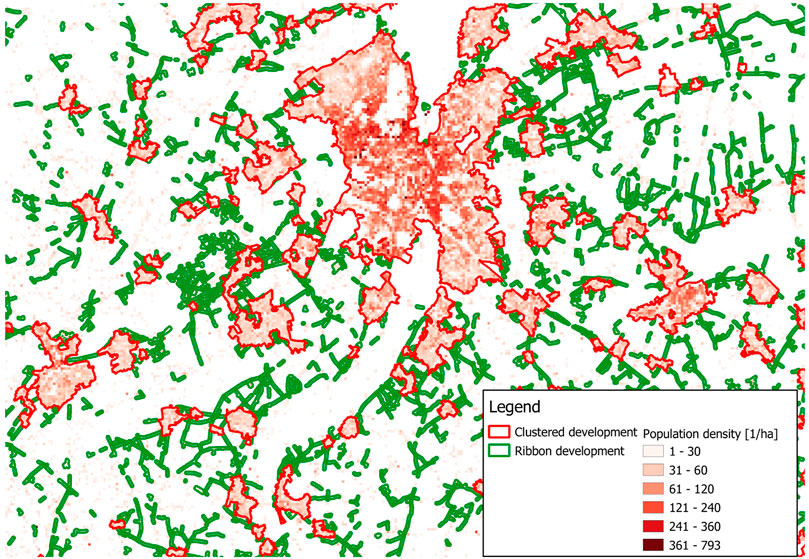
FIGURE 12. Cluster and ribbon development linked with population density.

4.2.2 Linking Kitchen and Garden Waste Data

In the case study region, kitchen and garden waste is collected door-to-door every 2 weeks. Figure 13 displays the collected waste on a monthly basis. The collected volumes are listed per collection round. Based on the coverage of both collection rounds, the number of rural and clustered building units per collection round are determined. Based on the average amount of kitchen and garden waste collected each month per collection round, the average mass of biowaste collected per building unit per month is quantified using Equation (4):

with w_c and w_r the average monthly biowaste collected per clustered and rural building unit and n_c,i and n_r,i the number of clustered and rural building units in collection area i, respectively. BW_tot,i is the total amount of biowaste that is collected on average each month in collection area i.

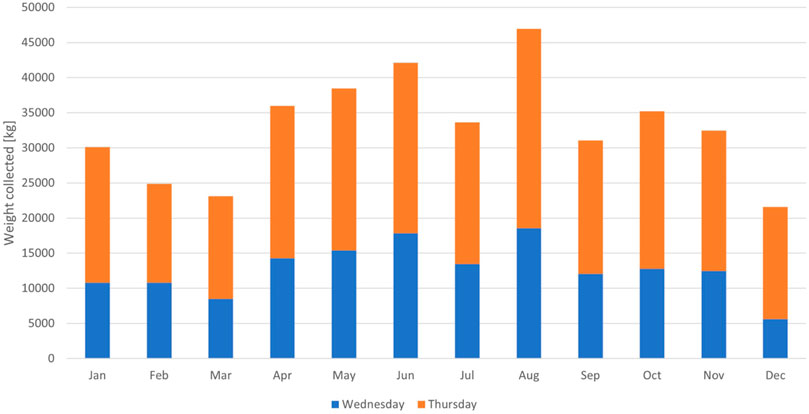
FIGURE 13. Monthly collection of kitchen and garden waste in the case study region: De Pinte, Flanders, Belgium.

One must note that the distinction between building units could be more detailed than the one presented. E.g., Vlaamse Overheid - Departement Omgeving - Afdeling Vlaams Planbureau voor Omgeving (2013a) lists the inhabitants density in Flanders per hectare in 2013. This information could be used to determine, per hectare, the average number of people living in a building unit. However, for this approach, the average amount of kitchen and garden waste produced per person per month has to be known. Most likely, an additional distinction will have to be made based on whether the person in question lives in a densely populated area or not. Unfortunately, at the time of writing this paper, this information was not available.

The proposed building clustering method, together with the monthly surface-area based biowaste quantification approach presented above has been applied for quantifying the yearly to-be-expected volumes of agricultural biowaste in the region of De Pinte, Belgium (see Section 5).

4.3 Towards Drafting an Optimal Small-Scale Biorefinery Design

The quantification methods presented in Sections 4.1 and 4.2 provide an estimation about the periodically available biowaste, from either agricultural or residential sources, in the considered collection area. The methods presented in this paper make up the bio-inventory tool of the decision support tool (DST) (Figure 1). The information obtained from the bio-inventory tool is fed to the process design tool and multi-objective optimisation tool in order to design an optimal small-scale biorefinery, specifically tailored for processing the locally available biowaste streams. The process design tool presently considers four process models that are particularly suited for a small-scale set-up: 1) Steam refining (Borrega et al., 2011a,b), 2) anaerobic digestion (Batstone et al., 2002; Nguyen, 2014), 3) ammonia stripping (Adu-Wusu et al., 2005; Değermenci et al., 2012), and 4) composting (Martalò et al., 2020). These process models rely on the amount of feedstock and its various characteristics to predict the outcome, hence, only the type of feedstock and its volume or flow is passed to the process design tool (Sbarciog et al., 2022). Based on the type of feedstock that is passed to a model, the conversion and quantification of the required feedstock properties is conducted in the preamble of each process. Although this method might seem fairly hard-coded at first hand, it offers a lot of flexibility with regard to combining different processes together whilst maintaining a small database. This significantly increases the speed of designing (multiple) suitable biorefinery process layouts.

As technical advances in decision support tools, process optimisation, and biorefineries are increasing rapidly, the decision support tool is developed using an open (-source) architecture, allowing for an easy extension of the tool’s capabilities employing other, already developed methods. For instance, the process model library can be easily extended with additional (kinetic) models of other biorefinery processes (De Buck et al., 2020; Sbarciog et al., 2022), or can be entirely circumvented by employing custom models. Using multi-platform communication techniques, e.g., INPROP (Muñoz López et al., 2018), the information on the available feedstocks provided by the bio-inventory tool can be passed to a stand-alone process simulator, like Aspen Plus, in order to simulate the performance of a custom/already existing biorefinery system. Moreover, complementing the optimisation approaches used in the DST, the eventually selected biorefinery design’s model can be employed for developing an optimal control strategy of the entire biorefinery system (Bhonsale et al., 2018).

5 Application to Case Study Region: De Pinte, Belgium

Figure 14 represents the case study region, with Figures 14A, B the building units and ground cover map of the studied area, respectively. The case study region has a surface area of 17.78 km² and has a maritime climate (Köppen classification Cfb).

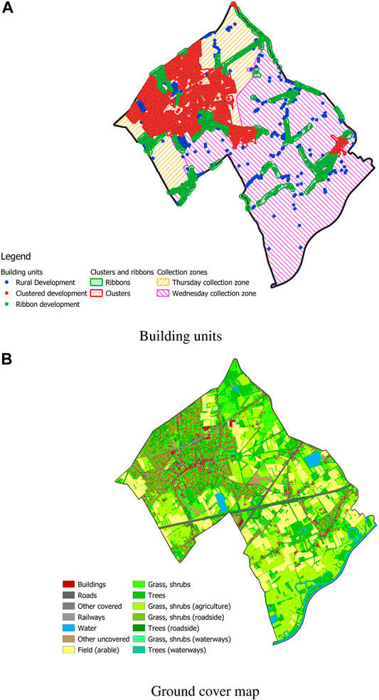
FIGURE 14. Building units with the two collection rounds and ground cover map of the case study region. (A) Building units, (B) Ground Cover map.

De Pinte counts a total of 5,016 clustered building units (i.e., building units located in a area dedicated as clustered or ribbon development) and 654 rural building units. The kitchen waste of 1768 of the clustered building units and 403 rural building units is collected on Wednesday on a biweekly basis, whereas the remainder of the building units’ kitchen waste is collected on Thursday on biweekly basis. Eq. (4) can therefore be translated into Equation (5):

The two collection areas are graphically represented in Figure 14A. Note that the Thursday collection area covers a smaller surface area, but one that is densely built-up. Solving the linear system of Eq. (5) renders w_c = 5.98 kg/month and w_r = 4.58 kg/month. One could argue that the obtained amounts for w_c and w_r are fairly small for one building unit per month. A first clarification for these low values is that the majority of building units in the case study region, for which the monthly collected amounts were available, are single household residences. Moreover, the linear system of Eq. (4) assumes that, during every biweekly collection round, biowaste is collected from every building unit that is called on during the collection round. In practice, however, not all building units on a collection round will have their kitchen and garden waste collected.

As kitchen waste has, on average, a high relative N-content, it is especially suited to be processed in an anaerobic digestion facility, combined with an ammonia stripping process. Note, however, as a C: N ratio between 20 and 30 is deemed to be the most favourable for a digestion process, it could be more preferable to mix the kitchen waste feedstock with other, e.g., more C-rich feedstocks (Nguyen, 2014). Additionally, as the water content of kitchen waste is fairly high, one must consider that this feedstock is more prone to rotting.

Using the colour clustering method, 19.10% of the surface area of the case study region is covered by arable land and 14.10% is covered in grassland for agricultural use, resulting in a surface area of 340 and 251 ha, respectively. Using the surface area-based biowaste quantification values defined in Section 4.1.2, this results in a maximum agricultural biowaste stream of 2,547 ton residue due to the cultivation of cereals per year and 1,125 ± 399 tons of dry grass per mowing cycle. For both residue streams, however, the remark should be made that they are not necessarily entirely harvested as residue streams. Corn stalks, e.g., are usually left in the soil to counteract soil erosion during the winter months (Renard et al., 1997). Dry grass, on the other hand, is usually harvested as fodder rather than being regarded as a waste stream.

These local exceptions highlight the necessity of a decision support tool taking the local setting into account as every local scenario is different. The decision support tool can provide a first, holistic overview of what is possible in a certain area, but even then, this information needs to be backed-up by expert knowledge on the availability of certain biowaste streams, etc.

6 Extendibility of the Presented Methods and Future Research

Both biowaste potential assessment methods have been developed with the future in mind, meaning that their extendibility and application potential to multiple feedstock types was an important development criteria. Especially with regard to the building clustering method, this approach can be easily extended to include other types of discrete and geographically spread feedstock production sites. For example, at the current point of development, agricultural waste is estimated using a surface area-based quantification approach. Farms, however, can also be identified as discrete points on a map from which a (steady) stream of biowaste can be expected. With regard to strengthening local collaborations between farmers that wish to process their biowaste in a more independent manner, the tool could easily be extended by adding a GIS-layer to the bio-inventory tool’s database that contains the considered farms and their periodic biowaste yields. When considering landscape maintenance in cities, for instance, GIS-layers containing the parks and natural city-scape elements, could be added to the bio-inventory tool database. Especially when these geographically spread biowaste production sites can be linked with in-depth expert knowledge on the type and amounts of biowaste that can be periodically harvested at each point, the proposed biowaste potential assessment methods provide a sturdy framework for developing and designing tailored biorefinery plants. With regard to the composition of the biowaste streams that can be quantified using the presented biowaste potential assessment approaches, the current bio-inventory toolbox is developed with a Flemish application area in mind. As biowaste collection in Flanders is characterised by a high level of waste sorting (both on size and type), the need for assessing the waste’s composition using the bio-inventory tool is non-existent as the collected biowaste streams of garden waste and kitchen waste can be assumed to have a uniform composition. Thus, at present, the main goal of the bio-inventory tool remains to assess quantities. For the composition of the biowaste, default compositions will be employed (Nguyen, 2014). However, if necessary, in the final DST, the decision maker will be able to complement the bio-inventory tool’s assessment of the biowaste potential of a certain area with their own data and knowledge.

The colour clustering method could additionally be further improved by considering different clustering algorithms. One of the main issues this approach currently faces, is the high level of noise on the data due to the overlapping of colours, potentially leading to a sub-optimal clustering of the currently employed k-means algorithm. Other clustering methods, like density-based clustering, have the advantage that they can distinguish clusters and noise from each other (Wang et al., 2018). Using similar methods, the true clusters centres could potentially be more accurately estimated by their capability of disregarding noise. Data points corresponding to the latter category can be attributed a posteriori to the already estimated clusters centres. However, as the clustering performance of the k-means algorithm with regard to the most prominent ground cover types/colours (i.e., those of interest) is satisfactory, the extension of the colour clustering method with additional clustering algorithms is set as a next step in the further development of the proposed biowaste potential assessment technique.

7 Conclusion

Biomass, and more specifically biowaste, can be used as a sustainable alternative feedstock for the production of energy and chemicals. To unlock the full potential of biowaste, however, it needs to be refined into manageable and value-added components. This is done in a biorefinery plant. Initial biorefinery plants were designed as bio-based copies of ordinary petroleum refineries, i.e., they were designed to compete with petroleum refineries for the production of fuels, etc., rather than as an environmentally friendly and vital alternative for the petroleum sector. These large-scale facilities mainly relied on the economy of scale to become economically viable enterprises and required large quantities of a uniform feedstock, often food-based. As these practices were, rightfully so, deemed to be ethically skewed as the more profitable energy industry started competing with the food industry for land, alternative feedstocks were sought in the form of biowaste. These streams could still be food-based but are no longer suitable for human consumption and/or do not compete with the food producing industry for arable land. Especially small-scale and locally embedded biorefineries are considered to be extremely suitable for processing these types of waste streams (Bruins and Sanders, 2012). In order to do so, however, the biorefinery plant needs to be maximally optimised and tailored to its local setting. For this, it is required to have a good understanding of the local setting that is considered, especially when it comes to the available biowaste streams types and their expected periodic volumes. This paper presents two biowaste potential assessment approaches, employing GIS techniques, for categorising and quantifying biowaste feedstocks: 1) the colour clustering method, using a ground cover map, and 2) the building units clustering method, using geographically spread data points representing biowaste production sites. Both methods are tailored for a Flemish (Belgian) setting and were applied to a local case study region: De Pinte. Both methods enable potential biorefinery exploiters to efficiently analyse the types and amounts of biowaste feedstocks that are present in the foreseen catchment area of the biorefinery. Using this information, an optimised biorefinery design can be drafted, especially tailored for the locally available feedstock. By doing so, the lack of confidence investors may have in these biorefinery processes may be eliminated by providing a in-depth, a priori, and in silico analysis of the overall sustainability of the presented biorefinery design in its local setting.

Data Availability Statement

The original contributions presented in the study are included in the article/Supplementary Material, further inquiries can be directed to the corresponding author.

Author Contributions

Conceptualisation: VDB, MS, MP, and JVI; investigation and literature review: VDB and MS; resources: VDB, MS, MP, and JVI; writing, original draft preparation: VDB; writing, review and editing: VDB, MS, MP, and JVI; visualisation: VDB; supervision: JVI; project administration: MP and JVI; funding acquisition: JVI.

Funding

This work was supported by the ERA-NET FACCE-SurPlus FLEXIBI Project, co-funded by VLAIO project HBC.2017.0176. This work was co-funded by the European Commission within the framework of the Erasmus+ FOOD4S Programme (Erasmus Mundus Joint Master Degree in Food Systems Engineering, Technology and Business 619864-EPP-1-2020-1-BE-EPPKA1-JMD-MOB). VDB is supported by FWO-SB Grant 1SC0922N.

Conflict of Interest

The authors declare that the research was conducted in the absence of any commercial or financial relationships that could be construed as a potential conflict of interest.

Publisher’s Note

All claims expressed in this article are solely those of the authors and do not necessarily represent those of their affiliated organizations, or those of the publisher, the editors and the reviewers. Any product that may be evaluated in this article, or claim that may be made by its manufacturer, is not guaranteed or endorsed by the publisher.

Acknowledgments

The authors would like to acknowledge the local council of De Pinte, Belgium, for their co-operation and the provision of the data necessary for this research.

References

Adu-Wusu, K., Martino, C., Wilmarth, W., Bennett, W., and Peters, R. (2005). “Modeling Air Stripping of Ammonia in an Agitated Vessel,” in Tech. Rep. WSRC-MS-2005-00685. Washington, D.C., U.S.: U.S. Department of Energy.
[Dataset] Agentschap Informatie Vlaanderen (2019). Bodembedekkingskaart (Bbk), 1m Resolutie, Opname 2015. Online.
[Dataset] Agentschap Informatie Vlaanderen (2021). Gebouwen- en adressenregister. Oxford: WFS. Online.
Ait Sair, A., Kansou, K., Michaud, F., and Cathala, B. (2021). Multicriteria Definition of Small-Scale Biorefineries Based on a Statistical Classification. Sustainability 13, 7310. doi:10.3390/su13137310
Álvarez del Castillo-Romo, A., Morales-Rodriguez, R., and Román-Martínez, A. (2018). Multiobjective Optimization for the Socio-Eco-Efficient Conversion of Lignocellulosic Biomass to Biofuels and Bioproducts. Clean. Techn Environ. Pol. 20, 603–620. doi:10.1007/s10098-018-1490-x
Angouria-Tsorochidou, E., Teigiserova, D. A., and Thomsen, M. (2022). Environmental and Economic Assessment of Decentralized Bioenergy and Biorefinery Networks Treating Urban Biowaste. Resour. Conservation Recycling 176, 105898. doi:10.1016/j.resconrec.2021.105898
Angouria-Tsorochidou, E., Teigiserova, D. A., and Thomsen, M. (2021). Limits to Circular Bioeconomy in the Transition towards Decentralized Biowaste Management Systems. Resour. Conservation Recycling 164, 105207. doi:10.1016/j.resconrec.2020.105207
Batstone, D. J., Keller, J., Angelidaki, I., Kalyuzhnyi, S. V., Pavlostathis, S. G., Rozzi, A., et al. (2002). The IWA Anaerobic Digestion Model No 1 (ADM1). Water Sci. Technol. 45, 65–73. doi:10.2166/wst.2002.0292
Bhonsale, S., Telen, D., Vercammen, D., Vallerio, M., Hufkens, J., Nimmegeers, P., et al. (2018). Pomodoro: A Novel Toolkit for Dynamic (MultiObjective) Optimization, and Model Based Control and Estimation All the authors are with KU Leuven - Department of Chemical Engineering, BioTeC & OPTEC, Gebroeders de Smetstraat 1, B-9000,Ghent, Belgium. IFAC-PapersOnLine 51, 719–724. doi:10.1016/j.ifacol.2018.03.122
Borrega, M., Nieminen, K., and Sixta, H. (2011a). Degradation Kinetics of the Main Carbohydrates in Birch wood during Hot Water Extraction in a Batch Reactor at Elevated Temperatures. Bioresour. Technol. 102, 10724–10732. doi:10.1016/j.biortech.2011.09.027
Borrega, M., Nieminen, K., and Sixta, H. (2011b). Effects of Hot Water Extraction in a Batch Reactor on the Delignification of Birch wood. BioResources 6, 1890–1903.
Boulamanti, A., and Moya, J. (2017). “Energy Efficiency and GHG Emissions: Prospective Scenarios for the Chemical and Petrochemical Industry,” in Tech. Rep. EUR 28471 EN (Maastricht, Netherlands: European Union). doi:10.2760/20486
Bruins, M. E., and Sanders, J. P. M. (2012). Small-scale Processing of Biomass for Biorefinery. Biofuels, Bioprod. Bioref. 6, 135–145. doi:10.1002/bbb.1319
Carroll, A., and Somerville, C. (2009). Cellulosic Biofuels. Annu. Rev. Plant Biol. 60, 165–182. doi:10.1146/annurev.arplant.043008.092125
Cherubini, F., Jungmeier, G., Wellisch, M., Willke, T., Skiadas, I., Van Ree, R., et al. (2009). Toward a Common Classification Approach for Biorefinery Systems. Biofuels, Bioprod. Bioref. 3, 534–546. doi:10.1002/bbb.172
Clauser, N. M., Gutiérrez, S., Area, M. C., Felissia, F. E., and Vallejos, M. E. (2016). Small-sized Biorefineries as Strategy to Add Value to Sugarcane Bagasse. Chem. Eng. Res. Des. 107, 137–146. doi:10.1016/j.cherd.2015.10.050
De Buck, V., Polanska, M., and Van Impe, J. (2020). Modeling Biowaste Biorefineries: A Review. Front. Sustain. Food Syst. 4, 11. doi:10.3389/fsufs.2020.00011
De Meyer, A., Cattrysse, D., and Van Orshoven, J. (2016). Considering Biomass Growth and Regeneration in the Optimisation of Biomass Supply Chains. Renew. Energ. 87, 990–1002. doi:10.1016/j.renene.2015.07.043
De Visser, C., and Van Ree, R. (2016). Small-Scale Biorefining. Washington, D.C., USA: Wageningen University & Research. Available at:(Accessed January 6, 2022).
Değermenci, N., Ata, O. N., and Yildız, E. (2012). Ammonia Removal by Air Stripping in a Semi-batch Jet Loop Reactor. J. Ind. Eng. Chem. 18, 399–404. doi:10.1016/j.jiec.2011.11.098
Elia, J. A., and Floudas, C. A. (2014). Energy Supply Chain Optimization of Hybrid Feedstock Processes: A Review. Annu. Rev. Chem. Biomol. Eng. 5, 147–179. doi:10.1146/annurev-chembioeng-060713-040425
[Dataset] Food and Agriculture Organization of the United Nations (2020). Cereal Yield (Kg Per Hectare). Rome, Italy: FAO. Online.
Geraili, A., Salas, S., and Romagnoli, J. A. (2016). A Decision Support Tool for Optimal Design of Integrated Biorefineries under Strategic and Operational Level Uncertainties. Ind. Eng. Chem. Res. 55, 1667–1676. doi:10.1021/acs.iecr.5b04003
Geraili, A., Sharma, P., and Romagnoli, J. A. (2014). Technology Analysis of Integrated Biorefineries through Process Simulation and Hybrid Optimization. Energy 73, 145–159. doi:10.1016/j.energy.2014.05.114
Glivin, G., Kalaiselvan, N., Mariappan, V., Premalatha, M., Murugan, P. C., and Sekhar, J. (2021). Conversion of Biowaste to Biogas: A Review of Current Status on Techno-Economic Challenges, Policies, Technologies and Mitigation to Environmental Impacts. Fuel 302, 121153. doi:10.1016/j.fuel.2021.121153
Green-Armytage, P. (2010). A Colour Alphabet and the Limits of Colour Coding. Colour: Des. creativity 5, 1–23.
Isikgor, F. H., and Becer, C. R. (2015). Lignocellulosic Biomass: a Sustainable Platform for the Production of Bio-Based Chemicals and Polymers. Polym. Chem. 6, 4497–4559. doi:10.1039/C5PY00263J
Jeevahan, J., Anderson, A., Sriram, V., Durairaj, R. B., Britto Joseph, G., and Mageshwaran, G. (2021). Waste into Energy Conversion Technologies and Conversion of Food Wastes into the Potential Products: a Review. Int. J. Ambient Energ. 42, 1083–1101. doi:10.1080/01430750.2018.1537939
Junqueira, T. L., Cavalett, O., and Bonomi, A. (2016). The Virtual Sugarcane Biorefinery-A Simulation Tool to Support Public Policies Formulation in Bioenergy. Ind. Biotechnol. 12, 62–67. doi:10.1089/ind.2015.0015
Kelly, K., and Judd, D. (1976). Color: Universal Language and Dictionary of Names. Washington, D.C., USA: U.S. Department of commerce.
Kolfschoten, R. C., Bruins, M. E., and Sanders, J. P. M. (2014). Opportunities for Small-Scale Biorefinery for Production of Sugar and Ethanol in the netherlands. Biofuels, Bioprod. Bioref. 8, 475–486. doi:10.1002/bbb.1487
Lemire, P. O., Delcroix, B., Audy, J. F., Labelle, F., Mangin, P., and Barnabé, S. (2019). Gis Method to Design and Assess the Transportation Performance of a Decentralized Biorefinery Supply System and Comparison with a Centralized System: Case Study in Southern Quebec, canada. Biofuels, Bioprod. Bioref. 13, 552–567. doi:10.1002/bbb.1960
Leong, H. Y., Chang, C.-K., Khoo, K. S., Chew, K. W., Chia, S. R., Lim, J. W., et al. (2021). Waste Biorefinery towards a Sustainable Circular Bioeconomy: a Solution to Global Issues. Biotechnol. Biofuels 14. doi:10.1186/s13068-021-01939-5
Martalò, G., Bianchi, C., Buonomo, B., Chiappini, M., and Vespri, V. (2020). Mathematical Modeling of Oxygen Control in Biocell Composting Plants. Mathematics Comput. Simulation 177, 105–119. doi:10.1016/j.matcom.2020.04.011
Martinkus, N., Latta, G., Rijkhoff, S. A. M., Mueller, D., Hoard, S., Sasatani, D., et al. (2019). A Multi-Criteria Decision Support Tool for Biorefinery Siting: Using Economic, Environmental, and Social Metrics for a Refined Siting Analysis. Biomass and Bioenergy 128, 105330. doi:10.1016/j.biombioe.2019.105330
Masson-Delmotte, V., Zhai, P., Pirani, A., Connors, S. L., Péan, C., Berger, S., et al. (2021). “IPCC, 2021: Climate Change 2021: The Physical Science Basis,” in Contribution of Working Group I to the Sixth (Cambridge: Cambridge University Press).
Mohr, A., and Raman, S. (2013). Lessons from First Generation Biofuels and Implications for the Sustainability Appraisal of Second Generation Biofuels. Energy Policy 63, 114–122. doi:10.1016/j.enpol.2013.08.033
Muñoz López, C. A., Telen, D., Nimmegeers, P., Cabianca, L., Logist, F., and Van Impe, J. (2018). A Process Simulator Interface for Multiobjective Optimization of Chemical Processes. Comput. Chem. Eng. 109, 119–137. doi:10.1016/j.compchemeng.2017.09.014
Naik, S. N., Goud, V. V., Rout, P. K., and Dalai, A. K. (2010). Production of First and Second Generation Biofuels: A Comprehensive Review. Renew. Sustain. Energ. Rev. 14, 578–597. doi:10.1016/j.rser.2009.10.003
Nguyen, H. (2014). “Modelling of Food Waste Digestion Using ADM1 Integrated with Aspen Plus,”. Ph.D. thesis (Southampton, England: University of Southampton).
Pedregosa, F., Varoquaux, G., Gramfort, A., Michel, V., Thirion, B., Grisel, O., et al. (2011). Scikit-learn: Machine Learning in python. J. machine Learn. Res. 12, 2825–2830.
QGIS Development Team (2021). QGIS Geographic Information System. Beaverton, Oregon, US: Open Source Geospatial Foundation.
Radford, K. J. (1979). A Model for Strategic Planning. INFOR: Inf. Syst. Oper. Res. 17, 151–165. doi:10.1080/03155986.1979.11731730
Renard, K., Foster, G., Weesies, G., McCool, D., and Yoder, D. (1997). “Predicting Soil Erosion by Water: a Guide to Conservation Planning with the Revised Universal Soil Loss Equation (RUSLE),” in Agricultural Handbook 703 (Washington, D.C., USA: US Department of Agriculture).
Sbarciog, M., De Buck, V., Akkermans, S., Bhonsale, S., Polanska, M., and Van Impe, J. (2022). Design, Implementation and Simulation of a Small Scale Biorefinery. Processes To be submitted.
Schröder, T., and Geldermann, J. (2019). Improving Planning by Integrating Spatial Data into Decision Support Systems. J. Decis. Syst. 28, 309–329. doi:10.1080/12460125.2019.1697144
Schröder, T., Lauven, L.-P., and Geldermann, J. (2018). Improving Biorefinery Planning: Integration of Spatial Data Using Exact Optimization Nested in an Evolutionary Strategy. Eur. J. Oper. Res. 264, 1005–1019. doi:10.1016/j.ejor.2017.01.016
Sharma, P., Sarker, B. R., and Romagnoli, J. A. (2011). A Decision Support Tool for Strategic Planning of Sustainable Biorefineries. Comput. Chem. Eng. 35, 1767–1781. doi:10.1016/j.compchemeng.2011.05.011
Sukumara, S., Faulkner, W., Amundson, J., Badurdeen, F., and Seay, J. (2014). A Multidisciplinary Decision Support Tool for Evaluating Multiple Biorefinery Conversion Technologies and Supply Chain Performance. Clean. Techn Environ. Pol. 16, 1027–1044. doi:10.1007/s10098-013-0703-6
Tay, D. H. S., NgNg, D. K. S., KheireddineKheireddine, H., and El-Halwagi, M. M. (2011). Synthesis of an Integrated Biorefinery via the C-H-O Ternary Diagram. Clean. Techn Environ. Pol. 13, 567–579. doi:10.1007/s10098-011-0354-4
Thiriet, P., Bioteau, T., and Tremier, A. (2020). Optimization Method to Construct Micro-anaerobic Digesters Networks for Decentralized Biowaste Treatment in Urban and Peri-Urban Areas. J. Clean. Prod. 243, 118478. doi:10.1016/j.jclepro.2019.118478
Van Meerbeek, K., Ottoy, S., De Meyer, A., Van Schaeybroeck, T., Van Orshoven, J., Muys, B., et al. (2015). The Bioenergy Potential of Conservation Areas and Roadsides for Biogas in an Urbanized Region. Appl. Energ. 154, 742–751. doi:10.1016/j.apenergy.2015.05.007
[Dataset] Vlaamse Overheid - Departement Landbouw en Visserij (2020). Landbouwgebruikspercelen Lv, 2020. Schaerbeek, Belgium: Vlaamse Overheid - Departement Landbouw en Visserij. Online.
[Dataset] Vlaamse Overheid - Departement Omgeving - Afdeling Vlaams Planbureau voor Omgeving (2013a). Inwonersdichtheid Per Ha Ruimtebeslag - Vlaanderen - Toestand 2013. Brussels, Belgium: Vlaamse Overheid - Departement Omgeving - Afdeling Vlaams Planbureau voor Omgeving. Online.
[Dataset] Vlaamse Overheid - Departement Omgeving - Afdeling Vlaams Planbureau voor Omgeving (2013b). Kernen, Linten, Verspreide Bebouwing in Vlaanderen. Brussels, Belgium: Vlaamse Overheid - Departement Omgeving - Afdeling Vlaams Planbureau voor Omgeving. Online.
Wang, J., Zhu, C., Zhou, Y., Zhu, X., Wang, Y., and Zhang, W. (2018). From Partition-Based Clustering to Density-Based Clustering: Fast Find Clusters with Diverse Shapes and Densities in Spatial Databases. IEEE Access 6, 1718–1729. doi:10.1109/ACCESS.2017.2780109
Wang, L., Agyemang, S. A., Amini, H., and Shahbazi, A. (2015). Mathematical Modeling of Production and Biorefinery of Energy Crops. Renew. Sustain. Energ. Rev. 43, 530–544. doi:10.1016/j.rser.2014.11.008
Keywords: decision support tool, biorefinery, small-scale, local, biowaste
Citation: De Buck V, Sbarciog M, Polanska M and Van Impe JF (2022) Assessing the Local Biowaste Potential of Rural and Developed Areas Using GIS-Data and Clustering Techniques: Towards a Decision Support Tool. Front. Chem. Eng. 4:825045. doi: 10.3389/fceng.2022.825045
Received: 29 November 2021; Accepted: 10 January 2022;
Published: 16 February 2022.
Edited by:
Edwin Zondervan, University of Twente, NetherlandsReviewed by:
Ana Inés Torres, Universidad de la República, UruguayCarina L. Gargalo, Technical University of Denmark, Denmark
Copyright © 2022 De Buck , Sbarciog , Polanska and Van Impe. This is an open-access article distributed under the terms of the Creative Commons Attribution License (CC BY). The use, distribution or reproduction in other forums is permitted, provided the original author(s) and the copyright owner(s) are credited and that the original publication in this journal is cited, in accordance with accepted academic practice. No use, distribution or reproduction is permitted which does not comply with these terms.
*Correspondence: Jan F.M. Van Impe, jan.vanimpe@kuleuven.be